An Evolutionary Algorithm to Track Changes of Optimum Value
Locations in Dynamic Environments
Victoria S. Aragón, Susana C. Esquivel
Departamento de Informática Universidad Nacional de San Luis San Luis, Argentina
Laboratorio de Investigación y Desarrollo en Inteligencia Computacional, (LIDIC)1
Ejército de los Andes 950
{vsaragon, esquivel}@unsl.edu.ar
1 The LIDIC is supported by the Universidad Nacional de San Luis and the
ANPCYT (National Agency to Promote Science and Technology).
ABSTRACT
Non–stationary, or dynamic, problems change over time. There exist a variety of forms of dynamism. The concept of dynamic environments in the context of this paper means that the fitness landscape changes during the run of an evolutionary algorithm. Genetic diversity is crucial to provide the necessary adaptability of the algorithm to changes. Two mechanism of macromutation are incorporated to the algorithm to maintain genetic diversity in the population. The algorithm was tested on a set of dynamic testing functions provided by a dynamic fitness problem generator. The main goal was to determinate the algorithm’s ability to reacting to changes of optimum values that alter their locations, so that the optimum value can still be tracked when dimensional and multimodal scalability in the functions is adjusted. The effectiveness and limitations of the proposed algorithm is discussed from results empirically obtained.
Keywords: Evolutionary Algorithm, Dynamic
Environments, Genetic Diversity, Macromutation Operators.
1. INTRODUCTION
In general, the conditions of an optimization problem changes by one of the following reasons or a combination of both [1]: 1) the objective function changes itself, 2) the constraints change. A change in the objective function appears when the purpose of the problem changes. Here conditions, which were considered desirable before, can turn out to be undesirable now and vice versa. Changes in constraints, which modify feasibility of solutions, are related to resources and their availability. Changes can be small or big, soft or abrupt, chaotic, etc. [15, 16]. When changes are big, abrupt or chaotic the similarity between solutions found so far and the new ones can be worthless. Even under these hard environments Evolutionary Computation (EC) offers advantages, which are absent in non-population-based heuristics, when we search for solutions to non-stationary problems. The main advantage relies in the fact that Evolutionary Algorithms (EAs) keep a population of solutions.
Consequently, facing the change, they allow moving from a solution to another one to determine if any of them are of merit in order to continue the search from them instead of from scratch [2].
An optimization algorithm when handling changes in non-stationary systems needs to attack two goals: detecting that a change in the environment has occurred, and reacting properly to the change so that the optimum can still tracked. The principal objective of this study is to provide an effective method to response to the changes once the changes are detected.
Goldberg and Smith [3], Cobb [4] and Grefenstette [5] initiated the research related to the behaviour of EAs on dynamic fitness functions between 1987 and 1992. Recently the interest in this area was dramatically incremented [6], [7], [8], [9], [10], [11], [12], [13], [14], and [15].
The paper is organised as follows. Section 2 presents a definition of the dynamic environments studied in this work. Section 3 describes the dynamic test functions used. Section 4 describes the EA characteristics. In section 5 the experiments performed are described. In section 6 results are discussed and finally this document shows our conclusions, current and future work.
2. DYNAMIC FITNESS PROBLEM DEFINITION
A general definition, which describes and characterises a dynamic fitness function, is introduced here. The approach we follow assumes that each dynamic function consists of a base static function and a sequence of dynamic functions obtained from that base function and the application of a set of dynamic rules.
Definition 1: Let ψ be the searching space, a
vector x&∈ Ψ and the time t ∈ N. A dynamic
fitness function DFt is defined as follows
otherwise
) , ), ( (
0 if ) (
1 t t t
t t
t
s ch x DF g DF
t x
fb
& &
− =
=
(I)
where fb0(x&) is the base static function with m
possible features to be modified. Function gt is a
function having as arguments the dynamic fitness
function at time t-1, a set cht of all possible changes
to be applied to that function at time t and a given
severity s of the change, and returns a new fitness
function at time t.
Definition 2: Function gt is more precisely
defined as follows:
(
)
(II) ) , ( _ _ _
, ), (
1 1
L ch DF on changes apply
s ch x DF g
t t t t t
t
−
− & =
where the first argument of apply_changes_on_DF
t-1
:
{
}
m
i n
j
j i
t c FL
ch
1 1
,
= =
= (III)
is an ordered set of size mxn of all possible changes
at time t. When building this set, ci indicates which
function characteristic changes and FLj indicates
which part of the DFt-1 landscape will be modified
within the ith characteristic.
The second argument L of
apply_changes_on_DFt-1, is a binary vector of
length mxn, that indicates which members of cht are
selected and which are not selected to modify DF.
The severity of the changesis denoted by st.
3. DYNAMIC TESTING FUNCTIONS
In this section we will see that the functions provided by the Test Problem Generator [16] belong to the dynamic functions defined in ( I ). In this case
we have, ψ = Rn the searching space, a vector x&∈
Rn and the time t ∈ N. The dynamic function DFt
is defined as in ( I ) with the following base static function:
(
)
(
)
− + + − ∗ −
= =1, 1 1 2 .... 2
)
( t n tni
i t
i t i k i
t x max H R x x x x
fb &
(IV)
As it is defined fbt, specifies a “field of cones”,
where k indicates the number of cones in the
environment and each cone is independently
specified by its location (x1i , x2i , …, xni), its height
Hi, and its slope Ri.
The components of the vector defining the cone
location are xij ∈ [-1,1]. Each of these cones is
combined together by means of the max function.
Each time it is called the generator creates a randomly generated morphology. The user specifies the range of random values for the height, slope and location of cones:
Hi∈ [Hbase, Hbase + Hrange], Ri∈ [Rbase, Rbase + Rrange] and xij∈ [-1,1] (V)
In this case, when building the set cht of all
possible changes, a given characteristic ci ∈ {height,
slope, location} (m = 3) and FLj indicate which of
the k cones of the DFt-1 landscape will be modified
within the ith characteristic.
Consequently, when apply_changes_on_DF
t-1
operates, the corresponding modifications in DF
will be done only for those characteristics in the
cones where Lj+k(i-1) = 1, in the binary vector L, for
1 ≤ i ≤ m, 1 ≤ j ≤ k.
In this way we can see that the generator allows changing height, slope and location of one or more cones in the field of cones, which represents the morphology of the fitness landscape.
The severity of changes can have many degrees, from 1.0 which corresponds to soft and/or small changes to a degree near to 4.0 for chaotic changes. The degree of the severity is calculated by using the logistic function:
) 1
( 1
1 −
− ∗ − ∗
=
= p p p
t Y A Y Y
s
where A is a constant indicating the degree of
severity of the characteristic (height, slope, or
location) that will be modified and Y
pis the
value of the logistic function at iteration p. For
more details see [16].
4. EVOLUTIONARY ALGORITHM CHARACTERISTICS
We chose an evolutionary algorithm, which combines various forms of macro mutation similar to both, the hyper-mutation and random immigrants initially designed by Grefenstette [5].
Representation
The population P is made of a constant number N of
chromosomes, that depends on the dimensionality of each studied function. Each individual consists of a single chromosome, where each gene is a real value in the interval [-1.0, 1.0] representing a coordinate in
the search space. That is the ith individual in the
population P, is represented by the chromosome:
Pi = 〈xi1, xi2, …, xir〉
where xij denotes the jth coordinate of the ith
individual with j = 1,…,r and r is the chromosome
length.
Operators
A set of conventional and specialized operators was used. Conventional operators are:
Selection: The parents for the mating pool were
selected by means of tournament selection.
Recombination: The arithmetic crossover is
used to exchange genetic material between parents.
The operator is applied with a Pcross probability.
Mutation: Uniform mutation is used and it is
applied with a Pmut probability. When an individual
chosen from the domain of the corresponding parameter (vector component).
Specialised operators for macromutation are:
Recrudescence: This operator increments the
probabilities of undergoing recombination and/or mutation for a part of the population. It is applied in
every generation with a probability Precru and
produces a radical genotypic reorganisation on the individuals where it is applied. These individuals are selected randomly with uniform probability.
Random immigrants: Individuals randomly
generated replace a percentage of the population.
Evolutionary Algorithm Pseudocode
The structure of the proposed evolutionary algorithms follows:
0. t = 0 /* initial generation */
1.Generate fbt function and set DFt = fbt
2.Initialise Pt /* initial population */
3.Evaluate Pt
4.while (actual_number-changes < =
total_number_changes) do
5. { 6. t = t + 1
7.Generate next population P’t using traditional
operators and recrudecence if appropriate
8. Evaluate P’t
9. Calculate _statistics of P’t
10. Remember_the_best_of_generation /*
elitism */
11. if (function_changes) then
12. {
13. Store_statistical_report
14. Build_vector_L
15. Apply_changes_on_DFt-1(ch, L) and
obtain new DFt
16. }
17. if (occured_changes) then
18. { Evaluate P’t with new DFt
19. Calculate _statistics of P’t
20. Remember_the_best_of_generation
/* elitism */
21. apply_random_inmigrants_operator
22. Evaluate P’t
23. Calculate _statistics of P’t
24. Remember_the_best_of_generation
/* elitism */ 25. Let Pt = P’t
26. }
27. } /* end while */
28. Report_ statistics
In line 11, function_changes is responsible to detect if a change in dynamic fitness function must occur. In our case changes occur at constant intervals, then this function only verifies if the generation number corresponds to one where the change must occurs. If a change must occur we store
in the L vector what changes are to be done and in
which cones on the landscape to apply them (see line 14). Then the apply_changes function obtains a new dynamic fitness function in line 15. In the line 17,
occured_changes tests if a change effectively had occurred, in which case the application of macromutation operators creates the necessary genetic diversity. This function determinates if a change has occurred in the same form that the function function_changes does it. Then a new generation begins and so on, until the end condition is reached.
5. EXPERIMENT DESCRIPTION
The parameter settings for the evolutionary algorithm and the function generator are described now.
Parameters of the Evolutionary Algorithm
Except population size, the parameter settings for the EA remained fixed throughout all experiments and all scenarios, and were determined as the best after a series of initial trials:
The population size |P| was set to 100, 150 and
200 individuals for 2, 5 and 10 dimensions
functions, respectively. Pcross and Pmut were fixed at
0.25 and 0.5, respectively. For recrudescence, Precru
was set to 0.2, and the augmented probabilities of crossover and mutation were fixed at 0.5 and 0.8,
respectively. Tournament size was the 10% of
population size. The percentage of random
immigrants was set to 30% of the population. Immigrants are inserted when a change was produced. The individuals to be replaced by immigrants are randomly selected with equal probability. A number of experiments were designed differing in the function selected and in the severity of the changes to perform on it. For each of these experiments 30 runs were performed with distinct initial population.
Parameters of the Function Generator
We have two sets of parameter settings: general and specific. Table 1 shows the general parameter settings for the generator on all functions.
Table 1. Parameter Settings for the Generator
Hbase Hrange Rbase Rrange
[image:3.595.83.270.255.648.2]30 70 1 12
[image:3.595.322.514.705.749.2]Table 2 shows the specific parameter setting for the generator, on all functions, for large and chaotic changes. The severity of changes was selected because we agree with Branke [2] in which small and frequent changes should be accounted by creating robust solutions for the algorithm, while large and infrequent changes should be handled by adaptation.
Table 2. Parameter setting for severity of changes
Parameters Large
Changes
Chaotic Changes
A 1.50 3.8
The constant A is used by the logistic function to determine the change severity. The values chosen
for A creates a degree of severity which produce
large and chaotic changes[15] (near to the upper
limit required by the generator). The Cstepscale
constant is used to move each coordinate on the range specified by the user.
We worked on different functions whose features of dimensionality and multimodality are indicated in table 3, where “#d-#c” indicates number of dimensions and the number of cones.
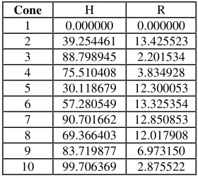
Because the generator randomly creates the functions, we adopted the following working
methodology. For example, for function f1 (see table
4), first we selected heights (H) and slopes (R) with the greatest multimodality. A similar table, not shown here for space limitations, is built for the 10 coordinates of each cone (the greatest dimensionality). The data associated with the experiments are available for any interested reader. This was done for each function.
Table 3. Functions used in the experiments
Functio n
#d-#c #d-#c #d-#c #d-#c #d-#c #d-#c
f1 2-5 2-10 5-5 5-10 10-5 10-10
f2 2-5 2-10 5-5 5-10 10-5 10-10
f3 2-5 2-10 5-5 5-10 10-5 10-10
[image:4.595.107.247.437.563.2]f4 2-5 2-10 5-5 5-10 10-5 10-10
Table 4. Initial Heights and Slopes for f1b0
Cone H R
1 0.000000 0.000000 2 39.254461 13.425523 3 88.798945 2.201534 4 75.510408 3.834928 5 30.118679 12.300053 6 57.280549 13.325354 7 90.701662 12.850853 8 69.366403 12.017908 9 83.719877 6.973150 10 99.706369 2.875522
When scalability is to be modified, to work with lower dimensions and lesser number of cones, we obtain the required values from these tables. For
example if we wish to work with f1 for 2-5, the
heights and slopes of the first five cones are retrieved from the table only for the first two dimensions of the coordinate’s table. Analogously we proceeded with the remaining functions. This working methodology allowed us to study the adaptability of the algorithm to changes and its behaviour, when facing scalability in space dimension and number of cones.
Changes were produced each 10, 50 and 70 generations for all functions. The main goal here was to determine if the algorithm succeeds to
faithfully track the change in location of the cone containing the optimum value when the fitness landscape changes. The algorithm was allowed to run as many generations as changes were desired to make. For all experiments we fixed at 20 the number of changes.
Types of Change
As it was mentioned the change in the location of the cone containing the optimum value is the only change analysed in the present work. Also experimentation was conducted with changes in the slope of one and all cones, but results showed that this type of changes were easy for the algorithms. For this reason they are not shown here.
Performance Metric
The following metric was used:
Accuracy (Acc) [17]: It is a metric specifically developed for non-stationary environments. It measures the average difference, between the best individual in the population at the generation “just before the change” and the optimal value, averaged to the number of changes. More precisely:
∑
=
−
= k
i
i b opt K
Acc
1
) (
1
where:
K is the number of changes suffered by the fitness
function.
opt is the mean value of optimal values found in
each change.
bi is the best value found before the ith change.
From its definition it is clear that small values of
the metric Acc indicate better results. A zero value
for accuracy means that the best individual in the population is found as the global optimum in every generation.
6. RESULTS
In first place, as our objective was analyse the macromutation operators we did a series of experiments with an EA without crossover operator. Tables 5 and 6 summarise the results obtained. In these tables entries (in bold) aligned with a percentage, indicate the number of runs where the algorithm detected a given percentage of changes.
CC indicates the percentage of changes detected by
the algorithm for each function. Acc indicates the
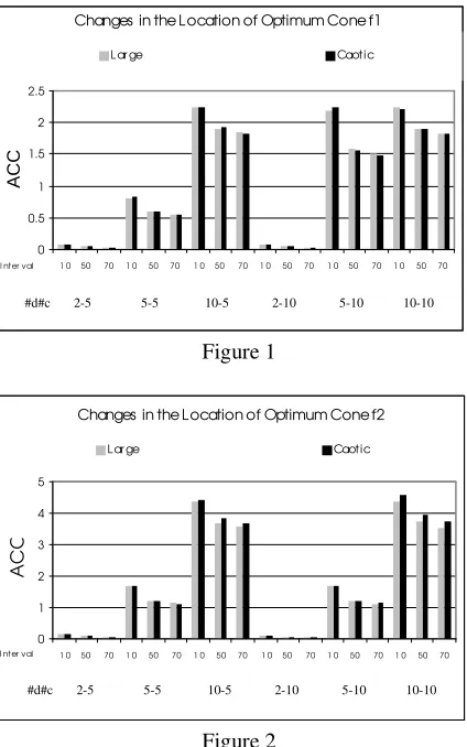
average mean values of accuracy for each function. Similarly, Figures 1 to 4 show the average mean values of accuracy over the 30 runs for each function.
From table 5 it can be observed that, the algorithm adapted for the 100% of changes for large changes and all 5-cone functions. A similar behaviour can be
seen for chaotic changes, except for function f4 in 10
Figure 1
Figure 2
Table 5. Percentage of large and chaotic changes
detected and average mean values for the performance metric on 5-cones landscapes dimensionally scaled.
Large Changes in the Location of Optimum Cone
2-5 5-5 10-5
Interval Interval Interval
f CC
10 50 70 10 50 70 10 50 70
100% 30 30 30 30 30 30 30 30 30
f1
Acc .09 .04 .03 0.84 0.61 0.55 2.24 1.93 1.86
100% 30 30 30 30 30 30 30 30 30
f2
Acc .17 .08 .06 1.67 1.2 1.15 4.39 3.7 3.58
100% 30 30 30 30 30 30 30 30 30
f3
Acc .31 .14 .13 2.98 2.21 2.0 7.89 6.64 6.4
100% 30 30 30 30 30 30 30 30 30
f4
Acc .36 .15 .13 3.14 2.24 2.07 8.24 6.89 6.61
Chaotic Changes in the Location of Optimum Cone
100% 30 30 30 30 30 30 30 30 30
Acc .09 .04 .03 .83 .61 0.55 2.24 1.92 1.82
100% 30 30 30 30 30 30 30 30 30
f2
Acc .17 .08 .07 1.68 1.21 1.13 4.44 3.85 3.7
100% 30 30 30 30 30 30 30 30 30
f3
Acc .32 .15 .13 3.04 2.24 2.03 8.29 7.0 6.82
100% 30 30 30 30 30 30 13 28 25
90% 11 2 5
80% 6
f4
Acc .35 .16 .13 3.05 2.19 2.04 8.35 7.11 6.9
10 generations) 80% of the changes were detected in 3 runs, 90% in 15 runs and 100% in 12 runs. It also can be observed that, as expected, as long as the interval between changes augmented the number of runs where the algorithm kept track of the 100% of changes, incremented as well. This allows us to conjecture that for a larger interval between changes the 100% of the cases could be detected in all runs.
We are trying to validate this conjecture through new experiments.
[image:5.595.313.524.214.386.2]From table 6 it can be observed that, the algorithm showed a robust behaviour keeping track of the 100% of the large and chaotic changes for all 10-cone functions.
Table 6. Percentage of large and chaotic changes
detected and average mean values for the performance metric on 10-cones landscapes dimensionally scaled.
Large Changes in the Location of Optimum Cone
2-10 5-10 10-10
Interval Interval Interval
f CC
10 50 70 10 50 70 10 50 70
100% 30 30 30 30 30 30 30 30 30
f1
Acc .09 .04 .03 2.24 1.6 1.48 2.27 1.95 1.87
100% 30 30 30 30 30 30 30 30 30
f2
Acc .11 .05 .04 1.66 1.2 1.13 4.36 3.72 3.55
100% 30 30 30 30 30 30 30 30 30
f3
Acc .31 .14 .13 3.0 2.22 1.99 7.93 6.6 6.41
100% 30 30 30 30 30 30 30 30 30
f4
Acc .14 .06 .05 0.77 0.55 0.51 4.5 3.81 3.67
Chaotic Changes in the Location of Optimum Cone
100% 30 30 30 30 30 30 30 30 30
f1
Acc .09 .04 .03 2.24 1.55 1.48 2.22 1.91 1.83
100% 30 30 30 30 30 30 30 30 30
f2
Acc .11 .05 .04 1.66 1.2 1.14 4.56 3.94 3.76
100% 30 30 30 30 30 30 30 30 30
f3
Acc .33 .14 .13 3.03 2.24 2.0 8.33 7.04 6.8
100% 30 30 30 30 30 30 30 30 30
f4
Acc .14 .06 .05 .79 .57 .53 4.66 3.99 3.86
Scalability Analysis at Dimensionality Level
Figures 1 to 4 indicate that, for a fixed number of
cones, accuracy P degrades when the dimensionality
[image:5.595.314.528.491.657.2]is augmented. Also, for a given dimensionality this metric improves its values as long as the interval between changes is incremented.
Figure 3
Scalability Analysis at Multimodality Level
By contrasting tables 5 and 6, we can see that for a given dimensionality, the behaviour of the algorithm
was very similar, except for the case of f4 with
chaotic changes. Here, the 5-dimensions functions showed to be harder than the 10-dimensions functions.
Changes in the Location of Optimum Cone f1
0 0.5 1 1.5 2 2.5
1 0 50 70 1 0 50 70 1 0 50 70 1 0 50 70 1 0 50 70 1 0 50 70 I nter val
ACC
L ar ge Caotic
Changes in the Location of Optimum Cone f2
0 1 2 3 4 5
1 0 50 70 1 0 50 70 1 0 50 70 1 0 50 70 1 0 50 70 1 0 50 70 I nter val
ACC
L ar ge Caotic
Changes in the Location of Optimum Cone f3
0 1 2 3 4 5 6 7 8 9
1 0 50 70 1 0 50 70 1 0 50 70 1 0 50 70 1 0 50 70 1 0 50 70 I nter val
ACC
L ar ge Caotic
#d#c 2-5 5-5 10-5 2-10 5-10 10-10
#d#c 2-5 5-5 10-5 2-10 5-10 10-10
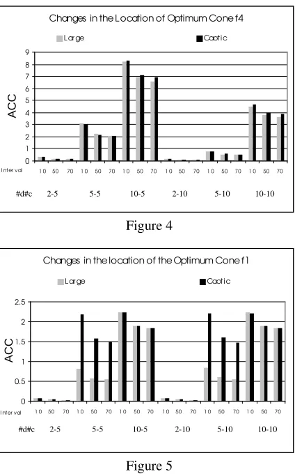
In a later study we prove the EA augmented with the crossover operator. The results are summarised in Figures 5 to 8. In these figures we can see that only in a few cases this operator allowed to improve the accuracy.
[image:6.595.311.525.71.230.2]With respect to the percentage of changes tracked the performance of both EAs (with and without crossover operator) was similar.
Figure 4
Figure 5
7. CONCLUSIONS
Results obtained by the proposed algorithm to track changes of optimum value locations are promising. The algorithm adapted to 100% of the changes (600 changes in 30 runs) for large changes in all proposed functions and under all studied conditions of multimodality and dimensionality. In the case of chaotic changes the behaviour was similar, except
for function f4 with higher multimodality, where it
was not successful to adapt to 100% of the changes. But indeed, under these conditions, it was able to track at least 100% of the changes in 13 runs, 90% (560 changes) in 11 runs and 80% (480) in 6 runs. The results showed that the principal operators were those that permitted to maintain genetic diversity, that is the macromutation operators.
In order to improve the performance of the algorithm under the hardest conditions, issues related to self-adaptation of operator probabilities will be considered. Presently we are working simultaneously in two problems: automatic detection
Figure 6
of changes and algorithm adaptability for tracking changes for the case where the height of the cone containing the optimum changes. We will continue experimentation scaling dimensionality and multimodality in functions generated with more controlled characteristics and not totally random, having in mind that the important issue here is not the accuracy achieved by the algorithm but its ability of creating at least one individual following the course towards the optimum.
Figure 7
Figure 8
Changes in the Location of Optimum Cone f4
0 1 2 3 4 5 6 7 8 9
1 0 50 70 1 0 50 70 1 0 50 70 1 0 50 70 1 0 50 70 1 0 50 70 I nter val
ACC
L ar ge Caotic
Changes in the Location of the Optimum Cone f2
0 1 2 3 4 5
1 0 50 70 1 0 50 70 1 0 50 70 1 0 50 70 1 0 50 70 1 0 50 70 I nter val
ACC
L ar ge Caotic
Changes in the Location of the Optimum Cone f3
0 1 2 3 4 5 6 7 8 9
1 0 50 70 1 0 50 70 1 0 50 70 1 0 50 70 1 0 50 70 1 0 50 70 I nter val
ACC
L ar ge Caotic
Changes in the location of the Optimum Cone f1
0 0.5 1 1.5 2 2.5
1 0 50 70 1 0 50 70 1 0 50 70 1 0 50 70 1 0 50 70 1 0 50 70 I nter val
ACC
L ar ge Caotic
Changes in the Location of the Optimum Cone f4
0 1 2 3 4 5 6 7 8 9
1 0 50 70 1 0 50 70 1 0 50 70 1 0 50 70 1 0 50 70 1 0 50 70 I nter val
ACC
L ar ge Caotic #d#c 2-5 5-5 10-5 2-10 5-10 10-10
#d#c 2-5 5-5 10-5 2-10 5-10 10-10
#d#c 2-5 5-5 10-5 2-10 5-10 10-10
#d#c 2-5 5-5 10-5 2-10 5-10 10-10
[image:6.595.70.282.176.516.2]8. REFERENCES
[1]Z. Michalewicz, and D.B. Fogel, - “How to
Solve It: Modern Heuristics”, Springer, 2000
[2]J. Branke, - “ Evolutionary Optimization in
Dynamic Environments”, Kluwer Academic Publishers, 2002.
[3]D. E. Golberg, and R. E. Smith,– “Nonstationary
Function Optimization using Genetic Algorithms with Dominance and Diploid”, Proceedings of the Second International Conference on Genetic Algorithms, pp. 59-68, Lawrence Erlbaum Associates, 1987.
[4]H.G. Cobb – “An Investigation into the use of
Hypermutation as an Adaptive Operator in Genetic Algorithms having Continuous, Time_Dependent Non-Stationary Environments”, Technical Report 6760, Naval Research Laboratory, USA, 1990.
[5]J. J. Grenfenstette,– “Genetic Algorithms for
Changing Environments”, Proceedings of the Second Conference on Parallel Problem Solving from Nature”, pp. 137 – 144, North Holland, 1992.
[6]N. S. Mori, et al. – “Adaptation to Changing
Environments by means of the Memory Based Thermodynamic Genetic Algorithm”, Proceeding of the Seventh International Conference on Genetic Algorithms, pp 299 – 306, Morgan Kaufmann, 1997.
[7]J. Lewis, E. Hart and G. Ritchie – “ A
Comparison of Dominance Mechanism and Simple Mutation in Non-Stationary Problems”, Proceeding of the Seventh International Conference on Genetic Algorithms, pp 138-148, Morgan Kaufmann, 1997.
[8]T. Bäck – “On the Behaviour of Evolutionary
Algorithms in Dynamic Fitness Landscapes”, Proceeding of IEEE International Conference on Evolutionary Algorithms, pp 446-451, IEEE Service Centre, 1998.
[9]C. O. Wile - “Evolutionary Dynamics in
Time-Dependent Environments”, PhD. Thesis, Institut für Neuroinformatik, Ruhr-Universität, Bochum, Germany, 1999.
[10]K. Trojanoswky and Z. Michalewicz –
“Searching for Optima in Non-Stationary Environments”, Proceeding of Congress on Evolutionary Computation, pp 1843-1850, IEEE Service Centre, 1999.
[11]K. Wicker and N. Weicker – “ On Evolutionary
Strategy Optimization in Dynamic Environments”, Proceeding of Congress on Evolutionary Computation, pp 2039-2046, IEEE Service Centre, 1999.
[12]W. Liles and K. De Jong. – “The Usefulness of
Tag Bits in Changing Environments”, Proceeding of Congress on Evolutionary Computation, pp 2054-2060, IEEE Service Centre, 1999.
[13]W.Yi, Q. Lin, and Y. He – “Dynamic
Distributed Genetics Algorithms”, Proceeding of Congress on Evolutionary Computation, pp 1132-1135, IEEE Service Centre, 2000.
[14]T. Nanayakkara, et al. – “ Adaptive
Optimization in a Class of Dynamic Environments using an Evolutionary Approach”, Journal of Evolutionary Computation, 7(1):45-68, 1999.
[15]R. W. Morrison – “ Designing Evolutionary
Algorithms for Dynamic Environments”, PhD Thesis, George Mason University, USA, 2002
[16]R.W. Morrison and K. De Jong – “A Test
Problem Generator for Non-Stationary Environments”, Proceedings of Congress on Evolutionary Computation, VIII, pp 2047 – 2053, Washington DC, USA, IEEE Service Center, 1999.
[17]K. Trojanowsky – “Evolutionary Algorithms