MPRA
Munich Personal RePEc Archive
Automatic Signal Extraction for
Stationary and Non-Stationary Time
Series by Circulant SSA
Juan B´
ogalo and Pilar Poncela and Eva Senra
Universidad de Alcal´
a, European Commission, Joint Research
Centre (JRC), Universidad de Alcal´
a
5 January 2017
Automatic Signal Extraction for Stationary and
Non-Stationary Time Series by Circulant SSA
Juan Bógalo
Universidad de Alcalá SPAIN
Pilar Poncela
European Commission, Joint Research Centre (JRC)
ITALY
Eva Senra
Universidad de Alcalá
SPAIN
January 5, 2017
Abstract
Singular Spectrum Analysis (SSA) is a nonparametric tecnique for signal extraction in time series based on principal components. However, it requires the intervention of the analyst to identify the frequencies associated to the extracted principal components. We propose a new variant of SSA, Circulant SSA (CSSA) that automatically makes this association. We also prove the validity of CSSA for the nonstationary case. Through several sets of simulations, we show the good properties of our approach: it is reliable, fast, automatic and produces strongly separable elementary components by frequency. Finally, we apply Circulant SSA to the Industrial Production Index of six countries. We use it to deseasonalize the series and to illustrate that it also reproduces a cycle in accordance to the dated recessions from the OECD.
Keywords: circulant matrices, signal extraction, singular spectrum analysis, non-parametric, time series, Toeplitz matrices.
JEL Classi…cation: C22, E32
1
Introduction
In many occasions, macroeconomic policy relies on analyzing a particular signal from the observed time series as the cycle or the trend. Additionally, statistical o¢ ces need to pro-duce seasonally adjusted data for a large amount of economic indicators. Singular Spectrum Analysis (SSA) is a non-parametric (and, therefore, model free) procedure based on sub-space algorithms for signal extraction. The main task in SSA is to extract the underlying components of a time series like the trend, cycle, seasonal and irregular components. It has been applied to a wide range of time series problems, besides signal extraction, like fore-casting, missing value imputation and others. SSA builds a trajectory matrix by putting together lagged pieces of the original time series and works with the Singular Value De-composition of this matrix. It is a procedure closely related to Principal Component (PC) analysis but applied to the trajectory matrix.
SSA has been applied in several …elds. In economics, Hassani and Thomakos (2010) review SSA for economic and …nancial time series, focusing on forecasting and the business cycle monitoring. Regarding forecasting, Hassani, Heravi, Brown and Ayoubkani (2013) and Silva and Hassani (2015) focus on the e¤ects of forecasting with SSA before and after the 2008 recession, Hassani, Soo… and Zhigljavsky (2013) forecast the in‡ation dynamics or Hassani, Heravi and Zhigljavsky (2013) forecast industrial production with multivariate SSA. Related to business cycles, de Carvalho, Rodrigues and Rua (2012) track the US busi-ness cycle, de Carvalho and Rua (2017) focus on the real time nowcasting of the output gap and Sella, Vivaldo, Groth and Ghil (2016) analyze economic cycles and their synchro-nization in three European countries. SSA has also been applied to estimate stochastic volatility models by Arteche and García-Enríquez (2016).
However, an important drawback of the initial SSA procedures is that the intervention of the analyst is required to identify the harmonic frequencies of the extracted components. To solve this problem we propose a new SSA methodology based on circulant matrices (CSSA). The main feature of these matrices is that their eigenstructure can be obtained as a function of the frequencies and therefore we can automatically identify the eigenvalues and eigenvectors associated to any particular frequency. Moreover, we also prove the validity of our proposal for nonstationary time series as well. An additional contribution of our method is the strong separability of the extracted components as compared to previous variants of SSA.
for signal extraction, without the intervention of the analyst, recovering reliable components that are strongly separable for both stationary and nonstationary time series.
The structure of this paper is as follows: Section 2 brie‡y describes the SSA technique. Section 3 proposes our new SSA procedure, named after Circulant SSA and proves its use for nonstationary time series too. Section 4 veri…es the strong separability of the extracted components. Section 5 presents a set of simulations to check the properties of the proposed methodology and Section 6 applies it to several real time series. Finally, Section 7 concludes.
2
SSA methodology
The origin of SSA dates back to 1986 with the publication of the papers by Broomhead and King (1986a, 1986b) and Fraedrich (1986). Vautard and Ghil (1989) introduce Toeplitz SSA under the assumption of stationary time series and Vautard et al. (1992) further develop the technique and are the …rst to derive an algorithm to obtain the extracted components with the length of the original series. At the same time, and independently, the so-called Caterpillar technique was developed in the former Soviet Union (see, Danilov and Zhigljavsky, 1997). Elsner and Tsonis (1996), Golyandina et al. (2001) and Golyandina and Zhigljavsky (2013) are books on the topic.
In this section we brie‡y describe the steps of the SSA technique to decompose a time series in its unobserved components. Let fxtg be a real valued time series of size T;
x= (x1; :::; xT)0;andLa positive integer, called the window length, such that1< L < T =2.
The Basic SSA or Broomhead-King (BK) procedure involves 4 steps: 1st step: Embedding
From the original time series we will obtain an L N trajectory matrix X given by L dimensional time series of length N =T L+ 1as
X= (x1j:::jxN) = 0 B B B B B @
x1 x2 x3 ::: xN
x2 x3 x4 ::: xN+1
..
. ... ... ... ... xL xL+1 xL+2 ::: xT
1 C C C C C A
wherexj = (xj; :::; xj+L 1)0 indicates the vector of dimensionLand origin at timej:Notice
that the trajectory matrixXis Hankel and both, by columns and rows, we obtain subseries of the original one.
In this step, we perform the singular value decomposition (SVD) of the trajectory matrixX=UD1=2V0 where Uis theL Lmatrix whose columns ukare the eigenvectors
of the second moment matrix S=XX0, D =diag( 1; :::; L), 1 ::: L 0, are the
eigenvalues of S and V is the N L matrix whose columns vk are the L eigenvectors of
X0X associated to nonzero eigenvalues. This decomposition allows to write X as the sum of the so-called elementary matricesXk of rank 1,
X=
r X
k=1
Xk= r X
k=1
ukw0k;
wherewk=X0uk=p kvk and r= max k>0fkg=rank(X). 3rd step: Grouping
Under the assumption of weak separability given in Golyandina et al. (2001), we group the elementary matrices Xk into m disjoint groups summing up the matrices within each
group. Let Ij = fj1; :::; jpg; j = 1; :::; m each disjoint group of indexes associated to the
corresponding eigenvectors. The matrixXIj =Xj1+:::+Xjp is associated to theIj group.
The decomposition of the trajectory matrix into this groups is given byX=XIj+:::+XIm:
The contribution of the component coming from matrixXIj is given by
P
k2Ij k=
Pr k=1 k:
4th step: Reconstruction
Let XIj = (xeij). In this step, each matrix XIj is transformed into a new time series
of the same length T as the original one, denoted as ex(j) = (xe1(j); :::;xe(Tj))0 by diagonal averaging of the elements ofXIj over its antidiagonals as follows
e
x(tj)=
8 > > < > > : 1 t Pt
i=1exi;t i+1; 1 t < L 1
L PL
i=1exi;t i+1; L t N 1
T t+1
PT N+1
i=L N+1exi;t i+1; N < t T
9 > > = > > ; :
The alternative Toeplitz SSA or Vautard-Ghil (VG) relies on the assumption that x
is stationary and zero mean and it performs the SVD decomposition in step 2 from an alternative matrixST= (sij) where
sij=
1 T ji jj
TXji jj
m=1
xmxm ji jj; 1 i; j L: (1)
In this case, the matrixST is the sample lagged variance-covariance matrix of the original
series, a symmetric Toeplitz matrix. The set ( k;uk;wk) is named the k-th eigentriple.
3
Circulant SSA
As previously stated in the introduction, a drawback of SSA in any of its variants is that it requires the intervention of the analyst to identify the harmonic frequencies of the extracted components. To try to overcome this problem, Ghil and Mo (1991), associate two di¤erent extracted principal components with similar eigenvalues to the same oscillation if they are highly correlated for a given lag. Vautard et al. (1992) suggest a test based on the periodogram to establish if a pair of eigenvectors are associated to the same harmonic. Later, Alexandrov and Golyandina (2004, 2005) introduce optimal thresholds for grouping eigenvectors linked to nearby frequencies in order to assign them to the same harmonic. Alonso and Salgado (2008) and Bilancia and Campobasso (2010) apply cluster techniques for grouping the elementary components based on k-means and hierarchical clustering, respectively. Nevertheless, whatever procedure is used, the grouping of frequencies is made after the elementary components are extracted. Also, the previous tests and procedures are based on parameters and/or thresholds that have to be previously set in a subjective way. Since the pairs of eigenvalues and eigenvectors are obtained, not as a function of the frequency, but rather on a decreasing magnitude, this means that the grouping is done with uncertainty. Bozzo et al. (2010) provided a partial solution by linking the eigenvalues-eigenvectors as a function of the frequency for symmetric positive de…nite Toeplitz matrices. However, the analytic form of the eigenvalues for this type of matrices is only known for heptadiagonal ones (see, Solary, 2013). We generalize this link between the eigenstructure and the associated harmonics by the use of circulant matrices.
In this section, we propose an automatic version of SSA based on circulant matrices. First, we deal with the stationary case and later on we will extend our proposal to the nonstationary case.
3.1 Stationary case
Toeplitz matrices appear when considering the population second order moments of the trajectory matrix. Let fxtg be an in…nite, zero mean stationary time series whose
autocovariances are given by m =E(xtxt m)m= 0;1; :::and its spectral density function,
a real2 -periodic, continuous function, denoted by f: Let
L(f) = 0 B B B B B @
0 1 2 ::: L 1 1 0 1 ::: L 2
..
. ... ... ... ...
L 1 L 2 L 3 ::: 0
1 C C C C C A (2)
be the L L matrix that collects the second moments. Notice that L(f) is a symmetric
Toeplitz matrix that depends on the spectral densityf through the covariances m. Recall that m = R01f(w) exp(i2 mw)dw for any integer m where w is the frequency in cycles per unit of time.
Analytic expressions for the eigenvalues of Toeplitz matrices are only known up to hep-tadiagonal matrices. To be able to have closed solutions of the eigenvalues and eigenvectors for any dimension, we use a special case of Toeplitz matrices that are the circulant ones. In a circulant matrix every row is a right cyclic shift of the row above as follows:
CL(f) = 0 B B B B B @
c0 c1 c2 ::: cL 1
cL 1 c0 c1 ::: cL 2
..
. ... ... ... ... c1 c2 c3 ::: c0
1 C C C C C A :
Following Lancaster (1969), thek-th eigenvalue of theL Lcirculant matrix CL(f) is
given by
L;k = LX1
m=0
cmexp i2 m
k 1 L
fork= 1; :::; L with associated eigenvector
uk=L 1=2(uk;1;:::; uk;L)0 (3)
whereuk;j = exp i2 (j 1)kL1 .
In particular, if we consider the circulant matrix of orderL Lwith elementscmde…ned
cm =
1 L
LX1
j=0
f j
L exp i2 m j
L ; m= 0;1; :::; L 1; (4) we have two interesting results. First, the eigenvalues of this circulant matrix coincide with the spectral density evaluated at pointsw= kL1,
L;k =f
k 1
L ; (5)
and second, the matrices L(f)andCL(f)are asymptotically equivalent asL! 1, L(f)
CL(f);in the sense that both matrices have bounded eigenvalues and lim L!1
k L(f)pCL(f)kF
L =
0, where k kF is the Frobenius norm, as Gray (1972; lemma 4.1) shows. Moreover, the eigenvalues of both matrices L(f) and CL(f) are asymptotically equally distributed in
the sense of Weyl1 as a consequence of the fundamental theorem of Szegö (Grenander and Szegö, 1958) as Trench (2003) shows.
To obtain a more operational version of the procedure, we consider a new circulant matrixCeL(f) whose elementsecm are given by
e
cm =
L m
L m+ m
L L m; m= 0;1; :::; L 1: (6) In this case, Pearl (1973) shows that L(f) is asymptotically equivalent to CeL(f): By
the transitivity property, the three matrices L(f), CeL(f) and CL(f) are asymptotically
equivalent.
Therefore, our proposal will consist on using these closed forms of the eigenvalues and eigenvectors to associate the SSA elementary components to a particular frequency before extracting them. Moreover, with this approach the spectral density is easily evaluated at frequencies kL1 by the eigenvalues of theCeL(f) matrix.
Finally, to deal with observed data we have to work with estimated, rather than popula-tion, quantities. So, we substitute the population autocovariancesf mgLm=01, by the sample second momentsfsmgmL=01 wheresm; m= 0; :::; L 1is de…ned as
sm =
1
T m
TXm
t=1
xtxt m:
1
Weyl de…nes two sets of bounded real numbersfan;kgnk=1andfbn;kgnk=1as asymptotically equally
distrib-uted if for a given continuous functionF on the interval[ K; K], it holds that lim
n!1
n P
k=1(
F(an;k) F(bn;k))
Since the sample autocovariances converge in probability to the population autocovariances, we de…neSC with elements given by
b
cm =
L m
L sm+ m
LsL m; m= 0;1; :::; L 1: (7) In what follows, we describe our new proposed algorithm, named Circulant SSA. Given the time series datafxtgTt=1:
1st step: Embedding. This step is as before.
2nd step: Decomposition. Compute the circulant matrix SC whose elements are
given in (7). Find the eigenvaluesbk ofSC and based on (5), associate the k-th eigenvalue
to the frequencyw= kL1; k= 1; :::; L:
3rd step: Grouping. Given the symmetry of the spectral density, we have that
bk = bL+2 k. Their corresponding eigenvectors given by (3) are complex, therefore, they
are conjugated complex by pairs, uk = uL+2 k where v indicates the complex conjugate
of a vectorv, and ukX and uL+2 kX correspond to the same harmonic period, where v
denotes the transpose conjugate ofuk . We proceed as follows to transform them in pairs
of real eigenvectors in order to compute the associated components.
To form the elementary matrices we …rst form the groups of 2 elementsBk=fk; L+ 2
kg fork= 2; :::; M withB1 =f1g and BL
2+1=
L
2 + 1 ifL is even. Second, we compute
the elementary matrix by frequency XBk as the sum of the two elementary matrices Xk
and XL+2 k, associated to eigenvalues bk and bL+2 k and frequency kL1,
XBk = Xk+XL+2 k
= ukukX+uL+2 kuL+2 kX
= (ukuk+ukuk)X
= 2(RukR 0
uk+IukI 0
uk)X
where the prime denotes transpose,Ruk denotes the real part ofuk and Iuk its imaginary
part. In this way, all the matricesXk; k= 1; :::; L;are real.
4th step: Reconstruction. As before.
Notice that the elementary reconstructed series by frequency can be automatically as-signed to a component according to the goal of our analysis.
3.2 Nonstationary case
show that Circulant SSA can be applied to nonstationary time series. The next theorem, a generalization of the analogous given by Gray (1974), provides the theoretical background needed to apply Circulant SSA to nonstationary time series.
Theorem 1 Let TL(s) be a sequence of Toeplitz matrices withs(w) a real, continuous and
2 -periodic, such that s(w) 0, where the equality is reached in a …nite number of points
H=fw0
i; i= 1; :::; lg. Given a …nite , consider the disjoint sets
i= w2 wi0 ai; w0i +bi js(w)
1
; ai; bi2R+; i= 1; :::; l
and let g(w) be a function de…ned as
g(w) =
(
f(w) = s(1w) if w =2 [li=1 i
hi(w) if w2 i
)
where hi(w) is any real valued bounded function continuous in i. Let Mhi = ess sup
hi <1 and mhi =ess inf hi=hi w
0
i ai =hi w0i +bi = :
Let L;k; k= 1; :::; L; be the eigenvalues of(TL(s)) 1 sorted in decreasing order and let
F(x) be a continuos function in hM1
s;maxiMhi
i
with Ms =ess sup s, then
lim L!1 1 L L X k=1
F(min( L;k;max(egk; ))) =
1
Z
0
F(g(w))dw; (8)
where egk are the values of g(kL1) sorted in descending order.
Proof: The proof is given in the Appendix.
In a similar way to Gray (1974), the theorem states that the sequence of eigenvalues of the sequence of matrices (TL(s)) 1 are asymptotically distributed (in the sense of Weyl)
as the eigenvalues of the sequence of matrices TL(g) up to a …nite value as L tends to
in…nity. Moreover, the matrices TL(g) CL(g) and by Szegö’s theorem, the eigenvalues
of the sequence of matrices TL(g) are asymptotically distributed as the eigenvalues of the
sequence of matricesCL(g) up to a …nite value asL tends to in…nity.
As a result, for a nonstationary series, the union of the estimation of the spectral density in a point of discontinuity with the estimations in the adjoint frequencies through segments is an easy way of building the functionshi:If all the functionshiare constant and equal to a
particular value …nite , we have the particular case proved in Gray (1974). Therefore, the generalization to functions hi allows a better approximation of the spectral density when
4
Separability of SSA
Separability of the elementary series as well as those grouped by frequencies is an as-sumption of SSA and should also be a characteristic of the estimated components. This characteristic is important since many signal extraction procedures assume zero correlation between their underlying components, whereas the estimated signals can be quite corre-lated. As Golyandina et al. (2001) point out the SSA decomposition can be successful only if the resulting additive components of the series are quite separable from each other. In this section, we …rst introduce the basic notions of separability and how it is measured. Af-terwards, we show that Circulant SSA produces component series that are highly separable outperforming alternative algorithms.
For a …xed window length L; given two series nx(1)t o and nx(2)t o extracted from the seriesfxtg, we say that they are weakly separable if both their column as well as row spaces
are orthogonal, that is X(1) X(2) 0 = 0L L and X(1)
0
X(2) = 0N N. Furthermore, we
say that two series nx(1)t o and nx(2)t oare strongly separable if they are weakly separable and the two sets of singular values of the trajectory matrices X(1) and X(2) are disjoint. When the trajectory matrix of the original time series has not multiple singular values or, equivalently, each elementary reconstructed series belongs to a di¤erent harmonic, strong separability is guaranteed according to the previous de…nition.
Usually, separability is measured in terms ofw-correlation (see, for instance, Golyandina et al., 2001, and Golyandina and Zhigljavsky, 2013), that it is given by
w
12 =
x(1);x(2) w x(1)
w x(1) w
;
where x(1);x(2) w = (x(1))0Wx(2) is the so called w-inner product and x(1) w =
q
x(1);x(1)
w
and W=diag(1;2; :::; L; :::; L
z }| {
T 2(L 1)times
; :::;2;1). Note that the window length L
To show that Circulant SSA produces components that are strongly separable, …rst no-tice that the real eigenvectorsp2Ruk and
p
2Iuk (linked to eigenvalues kand L+2 k,
re-spectively, k= L+2 k) are orthogonal and have information associated only to frequency k 1
L . Those are the only eigenvectors that have information related to this frequency.
As eigenvectors can be considered …lters, Kume (2013), these pair of eigenvectors extract elementary series linked to the same frequency without mixing harmonics of other frequen-cies. As a result, the two elementary series, when reconstructed in step 4, have spectral correlation close to 1 between them and close to zero with the remaining ones. Taking into account the pairs of reconstructed series per frequency, any grouping of the reconstructed series results in disjoint sets from the point of view of the frequency. Then, Circulant SSA produce components that are approximately strongly separable. In this case, the graph of thew-correlation matrix is black color in the main diagonal and white elsewhere as in the ideal case.
As we shall see in the simulation and in the empirical application, CSSA produces components that are more separable than previous alternatives os SSA, Basic and Toeplitz.
5
Simulations
In this section we compare the performance of our new proposal, Circulant SSA, with the competing SSA algorithms, i.e. Basic SSA and Toeplitz SSA for a linear as well as nonlinear time series model. We focus on two main aspects: reliability of the estimated components in …nite samples and separability.
5.1 Linear time series
The …rst model is a basic structural time series model
xt=Tt+ct+st+et (9)
where Tt is the trend component, ct is the cycle, st is the seasonal component and et is
the irregular component. We assume an integrated random walk for the trend (see Young 1984) given by
Tt = Tt 1+ t 1 (10)
with t N(0; 2):The cyclical and seasonal components are speci…ed according to Durbin and Koopman (2012), where the cycle is given by the …rst component of the bivariate VAR(1)
ct e
ct !
= c cos(2 wc) sin(2 wc) sin(2 wc) cos(2 wc)
!
ct 1
ect 1
!
+ "t
e"t !
(11)
with "t
e"t !
N(0; 2"I) and w1
c the period with wc 2 [0;1]. The seasonal component is
given by
st=
[s=2]
X
j=1
aj;tcos(2 wjt) +bj;tcos(2 wjt) (12)
withwj = js; j= 1; :::;[s=2]and sthe seasonal period, where [ ]is the integer part andaj;t
and bj;t are two independent random walks with noise variances equal to 2j: Finally, the
irregular component is white noise with variance 2e:All the components are independent of each other. We set c = 1;so the trend, cycle and seasonal components have a unit root. We consider that the series are monthly with s= 12 and cyclical period equal to w1
c = 48
months. The sample size is T = 193 and the noise variances of the di¤erent components are given by 2 = 0:00062, 2j = 0:0042, 2"= 0:0082 and 2e = 0:062:We choose as window length L = 48 following Golyandina and Zhigljavsky (2013), since L is multiple of the seasonal period, it is equal to the cyclical period and T 1 is multiple ofL:
The trend is related to the 0 frequency, the cycle to frequency 1/48 and the seasonal components to frequencies 1/12, 1/6, 1/3, 1/4, 5/12 and 1/2. Then, according to (5) and the symmetry of the spectral density, the trend is reconstructed with the eigentriple 1, the cyclical component with the eigentriples 2 and 48, and the seasonal components with the eigentriples 5, 9, 13, 17, 21, 25, 29, 33, 37, 41 and 45. For example, for the frequencyw= 121, we have that kL1 = 121 , and therefore, we sum the elementary componentsk= 4812 + 1 = 5 and L+ 2 k= 48 + 2 5 = 45.
If the procedure for signal extraction works well, the simulated component yt (yt can
be the trend, cycle or seasonal component) could be written as
yt=ybt+ut
whereut is the noise and bytis the extracted signal. Then, in the regression
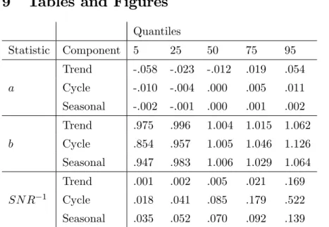
a = 0 (unbiasedness) and b = 1 (the scale is not changed). We simulate 1000 times the model and perform signal extraction with Circulant SSA. Table 1 shows the percentiles of the empirical distribution of the estimated coe¢ cients of the regression in (13). The last three rows of the table show the inverse of the signal to noise ratio
SN R 1=
2
u
2
s
where 2u is the variance of the noiseut= yt byt and 2s is the variance of the estimated
signal ybt. A value close to zero indicates that the explanatory power of the noise is very
small compared to that of the signal and it is an indication of a good approximation. Table 1 shows that the median of the estimated intercept and is almost zero for the three estimated components (cycle, seasonal component and trend). The median for the scale parameterbis almost one for the three components, but looking at the values for di¤erent quantiles, the empirical distribution for the estimatedb associated to the cycle indicates a larger dispersion.
TABLE 1 SHOULD BE INSERTED AROUND HERE
The estimated residuals from equation (9) are given by bet=xt Tbt bct bstand should
be white noise. In order to check this, we …t an AR(1) tobet. Table 2 shows the quantiles of
the empirical distribution of the mean, standard error and autoregressive coe¢ cient of the residuals of the 1000 replications. The median of the mean and autoregressive coe¢ cient are close to zero. The median of the standard deviation is 0.0529 (the value used for the simulations was 0.06).
TABLE 2 SHOULD BE INSERTED AROUND HERE
term of the estimated components. In Table 3 we present the summary statistics for the error term as well as the inverse of the SN R.
TABLE 3 SHOULD BE INSERTED AROUND HERE
Although the summary statistics from Table 3 seem to show that the three algorithms (Circulant, Basic and Toeplitz SSA) produce similar results, notice that Circulant SSA produces components with smallerSN R 1.
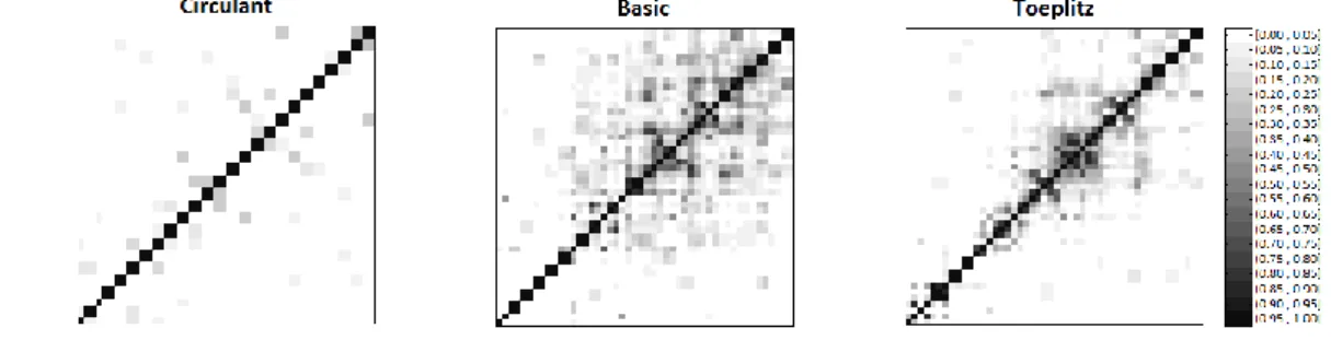
Regarding separability, Figure 1 plots the w-correlation matrices for the components extracted with the three algorithms. Notice that Circulant SSA produces matrices that are closer to diagonality than the other two alternatives where we can see di¤erent degrees of grey in the o¤-diagonal cells. Therefore, as it was expected, Circulant SSA recovers components that are more separable than the two alternative versions of SSA, Basic and Toeplitz.
FIGURE 1 SHOULD BE INSERTED AROUND HERE
5.2 Non-linear time series
For the case of non-linear time series, we borrow the model from Durbin and Koopman (2012) for UK travellers given by
xt=Tt+ct+ exp(a0+a1Tt) t+"t
where Tt is the trend, ct is the cycle and t is the seasonal component speci…ed as in
(10), (11) and (12), respectively. The parametersa0 anda1 are unknown …xed coe¢ cients.
Coe¢ cient a0 scales the seasonal component. The sign of the coe¢ cient a1 determines
whether the seasonal variation increases or decreases when a positive change in the trend occurs. The overall time varying amplitude of the seasonal component is determined by the combinationa0+a1 t:
As for the linear case, we simulate the model 1000 times for series of length T = 193 observations. We set a0 and a1 such that for each replication 0:5 exp(a0+a1 t) 1:5,
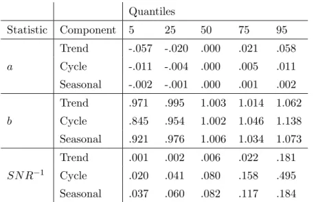
with a1 > 0. We apply Circulant SSA with a window length L = 48: Table 4 shows the
quantiles of the empirical distribution of the estimated coe¢ cients of the regression in (13). The last three rows of the table show the inverse of the signal to noise ratioSN R 1:
In order to check that the estimated residuals are white noise, we …t an AR(1) to bet as
in the linear case. Table 5 shows the quantiles of the empirical distribution of the mean, standard error and autoregressive coe¢ cient of the residuals of the 1000 replications. The median of the mean and autoregressive coe¢ cient are close to zero. The median of the standard deviation is 0.053 (the value used for the simulations was 0.06).
TABLE 5 SHOULD BE INSERTED AROUND HERE
As in the linear case, the results from the simulations seem very good. To compare Circulant SSA with alternative algorithms as Basic and Toeplitz SSA, we describe in more detail replication number 500. Table 6 shows the summary statistics of the residuals as well as the inverses of theSN Rin order to check the adequacy of the three versions of SSA.
TABLE 6 SHOULD BE INSERTED AROUND HERE
Although the three algorithms seem to work quite well, Circulant SSA produces compo-nents with smallerSN R 1. Figure 2 shows thew-correlation matrices for the components extracted with the three algorithms. Notice that in the nonlinear case, Circulant SSA also presents w-correlation matrices that are closer to the diagonality than the other two alter-natives where we can see di¤erent degrees of grey in the o¤-diagonal cells. Again, Circulant SSA recovers components that are more separable than the two alternative versions of SSA, Basic and Toeplitz.
FIGURE 2 SHOULD BE INSERTED AROUND HERE
6
Application
FIGURE 3 SHOULD BE INSERTED AROUND HERE
The …rst step is to establish the window length. Due to the monthly periodicity and seasonality, we select a window length multiple of 12. Assuming that the period of the cycle in these series goes from 1 year and a half to 8 years, we choose a window length multiple of 8 12=96 months. From the two available options, 96 and 192 months, we select the second one since it is larger according to the asymptotic results provided in Section 3.
We apply Circulant SSA, and associate the trend to the frequencies w = 0 and w = 1=192 (as they correspond to periods of in…nite and a long cycle of 16 years respec-tively). According to (5) and the symmetry of the spectral density, the trend is re-constructed with the eigentriples 1, 2 and 192 and with the elementary groups by fre-quencies B1 and B2 respectively. According to the assumption that the period for the
cycle goes from 1.5 to 8 years, this component is associated to the frequencies w = 1=96;1=64;1=48;5=192;1=32;7=192;1=24;3=64;5=96 and the cycle signal is reconstructed with the eigentriples 3 to 11 and 183 to 191, with the elementary groups by frequen-cies from B3 to B11: Finally, the seasonal component is associated to the frequencies
w= 1=12;1=6;1=4;1=3;5=12;1=2 and reconstructed in a similar way with the eigentriples 17, 33, 49, 65, 81, 97, 113, 129, 145, 161 and 177 and with the elementary groups by frequenciesB17; B33; B49; B65; B81;and B97:
Table 7 shows the contributions of the signals to the original IP variations in percentage. First, we highlight that the contribution of the irregular component (those oscillations not explained by the trend, cyclical or seasonal components) is smaller than 3.5% in all the countries. Main contributions come from the trend and seasonality, that account for more than 84% in all the countries. As expected, the contribution of the seasonal component is almost negligible in USA, and quite small in Japan and Germany, while it is very relevant in Italy and France. Finally, the cycle contributes in a range between 7.8% in Italy to 13.8% in Japan.
TABLE 7 SHOULD BE INSERTED AROUND HERE
Figure 3 shows the estimated trends for every country. The trend is a smooth component that has shown a decreasing evolution since the last decade for France, Italy and UK as a consequence of the last economic crisis. On the contrary, in Germnay and US, the trend shows an upward evolution in all the sample period.
cycle for all countries.
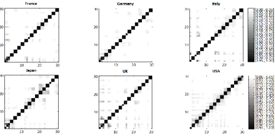
FIGURES 4 AND 5 SHOULD BE INSERTED AROUND HERE
Figure 5 shows the matrices of w-correlations and it can be seen that, as expected, Circulant SSA produces components that are strongly separable. Separability results is a very desirable feature in the construction of seasonal adjusted time series, that is the absence of any remaining seasonality. To check the quality of seasonal adjustment by Circulant SSA, we have applied the combined test for seasonality (Lothian, 1978) used in X12-ARIMA. We found that there were no signs of any remaining seasonality in any of the seasonal adjusted time series for the di¤erent countries2.
7
Conclusions
SSA is a nonparametric technique to extract the unobserved components present in a time series. Up to now, the intervention of the analyst was needed to identify the frequencies associated to each component. In this paper, we propose a new version of SSA, Circulant SSA, that does not need the intervention of the analyst. It relies on the asymptotic equiva-lence between Toeplitz and circulant matrices of second order moments of time series. The properties of circulant matrices allow to estimate the spectral density of a time series at certain frequencies through the eigenvalues. We can also identify automatically and a priori the frequencies associated to those eigenvalues. In this way, results are obtained very fast and with no subjective intervention from the analyst.
We also extend the algorithm to the nonstationary case providing a generalization of Gray’s theorem (1974).
The eigenvectors obtained from the diagonalization of the circulant matrix associated to second moments of the original series are real and form an orthonormal basis in the column space of the trajectory matrix. As a result, we can guarantee that all the elemental components are real. Additionally, they are strongly separable, so it is easy to group the elemental series to obtain the di¤erent signals (trend, cycle, seasonality...). We have compared our version of SSA to two already available ones (Basic and Toeplitz SSA) and although the …nal results are quite similar, Circulant SSA is faster, automatic and produces more separable components.
The properties of Circulant SSA have been checked through a set of simulations for linear and nonlinear time series models as well as through the empirical application where we showed that Circulant SSA produced deseasonalize series clean of any seasonality. The cycle was also very useful to study the business cycle.
8
Appendix
Proof of Theorem 1: As de…ned, the function g(w) is real, continuous and 2 -periodic. Its image is hM1
s;maxiMhi
i
being di¤erent from zero in the whole interval. Then, by the properties of the inverse of Toeplitz matrices TL(g 1)
1
TL(g). Moreover, if
F(x) is continuos inhM1
s;maxiMhi
i
, then F(1x)is continuos inhmax1
iMhi; Ms
i
:Given that Gutiérrez and Gutiérrez (2012) relax the assumption ofg(w)being a Wiener’s class function to a continuous and 2 -periodic function, Szegö’s Theorem leads to (8).
References
[1] Alexandrov, T. and Golyandina, N. (2004). The automatic extraction of time series trend and periodical components with the help of the Caterpillar-SSA approach. Ex-ponenta Pro, 3-4, 54-61.
[2] Alexandrov, T. and Golyandina, N. (2005). Automatic extraction and forecast of time series cyclic components within the framework of SSA. Proceedings of the Fifth Work-shop on Simulation, 45–50.
[3] Alonso, F.J. and Salgado, D.R. (2008). Analysis of the structure of vibration signals for tool wear detection. Mechanical Systems and Signal Processing, 22 (3), 735-748. [4] Arteche, J., and García-Enríquez, J. (2016). Singular Spectrum Analysis for signal
extraction in Stochastic Volatility models. Econometrics and Statistics.
[5] Bilancia, M. and Campobasso, F. (2010). Airborne particulate matter and adverse health events: robust estimation of timescale e¤ects. In Classi…cation as a Tool for Research, 481-489. Springer Berlin Heidelberg.
[7] Broomhead, D. and King, G. (1986a). Extracting qualitative dynamics from experi-mental data. Physica D, 20, 217–236.
[8] Broomhead, D. and King, G. (1986b). On the qualitative analysis of experimental dy-namical systems. In Nonlinear Phenomena and Chaos, 113–144. A. Hilger ed., Bristol. [9] Danilov, D. and Zhigljavsky, A. (editors) (1997). Principal components of time series:
the “Caterpillar” method. Saint Petersburg Press, Saint Petersburg (in Russian). [10] de Carvalho, M., Rodrigues, P. C., & Rua, A. (2012). Tracking the US business cycle
with a singular spectrum analysis. Economics Letters, 114(1), 32-35.
[11] de Carvalho, M., and Rua, A. (2017). Real-time nowcasting the US output gap: Sin-gular spectrum analysis at work. International Journal of Forecasting. 33 (1), 185–198. [12] Durbin, J. and Koopman, S.J. (2012). Time Series Analysis by State Space Methods.
Second edition. Oxford University Press.
[13] Elsner, J.B. and Tsonis, A.A. (1996). Singular spectrum analysis: a new tool in time series analysis. Plenum, New York.
[14] Fraedrich, K. (1986). Estimating the dimension of weather and climate attractors. Journal of the Atmospheric Sciences, 43 (5), 419–432.
[15] Ghil, M. and Mo, K. (1991). Intraseasonal oscillations in the global atmosphere. Part I and Part II, Journal of the Atmospheric Sciences, 48 (5), 752-790.
[16] Golyandina, N., Nekrutkin, V. and Zhigljavsky, A. (2001). Analysis of Time Series Structure: SSA and Related Techniques. Chapman & Hall/CRC.
[17] Golyandina, N. and Zhigljavsky, A. (2013). Singular Spectrum Analysis for Time Series. Springer.
[18] Gray, R.M. (1972). On the Asymptotic Eigenvalue Distribution of Toeplitz Matrices. IEEE Transanctions on Information Theory, 18 (6), 725–730.
[19] Gray, R.M. (1974). On Unbounded Toeplitz Matrices and Nonstationary Time Series with an Application to Information Theory. Information and Control, 24, 181–196. [20] Grenander, U. and Szegö, G. (1958). Toeplitz Forms and Their Applications. University
[21] Gutiérrez-Gutiérrez, J., and Crespo, P. M. (2012). Foundations and TrendsR in Com-munications and Information Theory. Foundations and TrendsR in Communications and Information Theory, 8(3), 179-257.
[22] Hassani, H., Heravi, S., Brown, G., and Ayoubkhani, D. (2013). Forecasting before, during, and after recession with singular spectrum analysis. Journal of Applied Statis-tics, 40(10), 2290-2302.
[23] Hassani, H., Heravi, S., and Zhigljavsky, A. (2013). Forecasting UK industrial pro-duction with multivariate singular spectrum analysis. Journal of Forecasting, 32(5), 395-408.
[24] Hassani, H., Soo…, A. S., and Zhigljavsky, A. (2013). Predicting in‡ation dynamics with singular spectrum analysis. Journal of the Royal Statistical Society: Series a (Statistics in Society), 176 (3), 743-760.
[25] Hassani, H., Thomakos, D. (2010). A review on singular spectrum analysis for economic and …nancial time series. Statistics and its Interface, 3(3), 377-397.
[26] Kume, K. (2013). Interpretation of singular spectrum analysis as complete eigen…lter decomposition. Advances in Adaptive Data Analysis, 4 (4).
[27] Lancaster, P. (1969). Theory of Matrices. Academic Press, NY.
[28] Lothian, J. (1978). The Identi…cation and Treatment of Moving Seasonality in the X-11 Seasonal Adjustment Method. StatCan Sta¤ Paper STC0803E, Seasonal Adjustment and Time Series Analysis Sta¤, Statistics Canada, Ottawa.
[29] Pearl, J. (1973). On Coding and Filtering Stationary Signals by Discrete Fourier Trans-form. IEEE Trans. on Info. Theory, IT-19, 229–232.
[30] Sella, L., Vivaldo, G., Groth, A., and Ghil, M. (2016). Economic cycles and their synchronization: a comparison of cyclic modes in three European countries. Journal of Business Cycle Research, 12(1), 25-48.
[31] Silva ES, andHassani H. (2015). On the use of singular spectrum analysis for forecasting U.S. trade before, during and after the 2008 recession. International Economics. [32] Solary, M.S. (2013). Finding eigenvalues for heptadiagonal symmetric Toeplitz
[33] Trench, W.F. (2003). Absolute equal distribution of the spectra of Hermitian matrices. Linear Algebra and its Applications, 366, 417-431.
[34] Vautard, R. and Ghil, M. (1989). Singular spectrum analysis in nonlinear dynamics, with applications to paleoclimatic time series. Physica D, 35, 395–424.
[35] Vautard, R., Yiou, P. and Ghil, M. (1992). Singular-spectrum analysis: A toolkit for short, noisy chaotic signal. Physica D, 58, 95–126.
9
Tables and Figures
Quantiles
Statistic Component 5 25 50 75 95 Trend -.058 -.023 -.012 .019 .054 a Cycle -.010 -.004 .000 .005 .011 Seasonal -.002 -.001 .000 .001 .002 Trend .975 .996 1.004 1.015 1.062 b Cycle .854 .957 1.005 1.046 1.126 Seasonal .947 .983 1.006 1.029 1.064 Trend .001 .002 .005 .021 .169 SN R 1 Cycle .018 .041 .085 .179 .522 Seasonal .035 .052 .070 .092 .139
Table 1. Statistics related to the goodness of …t of the extracted signals. The …rst columns are quantiles of the empirical distribution of the estimated coe¢ cients of the re-gression of the generated components over the extracted ones; the last three rows show the inverse of the signal to noise ratio.
Quantiles
Statistic 5 25 50 75 95 Mean -.003 -.001 .000 .001 .003 S.E. .048 .051 .053 .055 .058 -.173 -.083 -.031 .028 .117
Table 2. Quantiles of the empirical distribution of the statistics related to the residuals.
Statsitics for bet SN R 1
Algorithm Average S.E. Trend Cycle Seas Circulant .004 .053 -.063 .0008 .0133 .0586 Basic -.001 .053 -.073 .0014 .0140 .0599 Toeplitz .001 .054 -.059 .0008 .0194 .0651
Table 3. Summary statistics of the residuals of the model bet (columns 2 to 4) and
Quantiles
Statistic Component 5 25 50 75 95 Trend -.057 -.020 .000 .021 .058 a Cycle -.011 -.004 .000 .005 .011 Seasonal -.002 -.001 .000 .001 .002 Trend .971 .995 1.003 1.014 1.062 b Cycle .845 .954 1.002 1.046 1.138 Seasonal .921 .976 1.006 1.034 1.073 Trend .001 .002 .006 .022 .181 SN R 1 Cycle .020 .041 .080 .158 .495 Seasonal .037 .060 .082 .117 .184
Table 4. Statistics related to the goodness of …t of the extracted signals for the nonlinear model. The columns are quantiles of the empirical distribution of the estimated coe¢ cients of the regression of the generated components over the extracted ones; the last three rows show the inverse of the signal to noise ratio.
Quantiles
Statistic 5 25 50 75 95 Mean -.004 -.001 .000 .001 .003 S.E. .048 .051 .053 .055 .059 -.166 -.089 -.026 .029 .104
Table 5. Quantiles of the empirical distribution of the statistics related to the residuals.
Statsitics for bet SN R 1
Algorithm Average S.E. Trend Cycle Seas Circulant -.001 .054 -.145 .0020 .0315 .0372 Basic .002 .054 -.148 .0027 .0318 .0403 Toeplitz .000 .059 -.228 .0021 .0433 .0628
Table 6. Summary statistics of the residuals of the nonlinear model bet (columns 2 to
Components France Germany Italy Japan UK USA
Trend 52.1 77.3 42.7 79.0 72.0 87.9
Cycle 9.5 12.6 7.8 13.8 11.1 10.3
Seasonal 35.6 6.7 47.3 5.1 13.5 0.3
Irregular 2.8 3.4 2.2 2.1 3.4 1.5
Total 100.0 100.0 100.0 100.0 100.0 100.0
Figure 1: Example: w-correlations of the extracted components with Circulant, Basic and Toeplitz SSA.
Figure 2: Illustrative example: w-correlations of the extracted components with Circulant, Basic and Toeplitz SSA (nonlinear case).
Figure 4. Estimated cycles and OECD announced recessions (shadowed areas).