DEPARTAMENTO
DE
GEOGRAFÍA
–
UNIVERSIDAD
DE
ALCALÁ
BURN SEVERITY ESTIMATION FROM
REMOTELY SENSED DATA USING
SIMULATION MODELS
Tesis doctoral presentada por
Angela DE SANTIS
bajo la dirección del
Dr. Emilio CHUVIECO SALINERO
Catedrático de Análisis Geográfico Regional
AGRADECIMIENTOS
En primer lugar quiero agradecer a mi director de tesis, Emilio Chuvieco, por haberme dado la posibilidad de formar parte del grupo de investigación del Departamento de Geografía hace cuatro años. Sin temor a exagerar, puedo decir que esta decisión cambió toda mi vida. En estos años me ha demostrado siempre un gran apoyo y ha sido para mí una guía y un ejemplo a seguir.
Otro agradecimiento especial es para Javier Salas. Gracias a su ayuda he podido conseguir mi beca/contrato y he sobrevivido al “largo y tedioso” proceso de homologación de mi título de licenciada. Además le agradezco su amistad y disponibilidad infinita.
Gracias a Pilar Martín, por “los juguetes radiométricos”, las imágenes SPOT de Galicia, y sobre todo por estar a mi lado.
También me gustaría agradecer al resto de los profesores del Departamento por hacerme sentir parte de este maravilloso grupo de profesionales.
Siempre en el ámbito de la Universidad, quiero agradecer de corazón a todos mis compañeros (más conocidos como el “comando tupper”), por compartir conmigo alegrías y angustias, trabajo de campo y “momentos tupper”. Gracias chicos!
Además me gustaría dar las gracias a José Ángel, el forestal que ha sido mi “ángel de la guarda” en el trabajo de campo en el incendio de Guadalajara, y os puedo asegurar que lo necesitaba!
Ya a nivel personal, quiero agradecer a mis padres y a toda mi familia todos sus esfuerzos. Siempre han estado a mi lado, anteponiendo mi felicidad a las ganas de tenerme cerca. Han seguido cada paso de mi vida, apoyándome pero dejándome libre de decidir. Lo que soy y lo que estoy consiguiendo se lo debo a ellos. No creo que existan palabras que puedan expresar del todo lo que significan para mí.
Un lugar especial en estos agradecimientos es para Patrick. Gracias por estar a mi lado siempre, por tus ánimos en los momentos difíciles, por alegrarte conmigo en los buenos momentos, por tus consejos personales y profesionales, por las revisiones de los artículos, por tu ayuda en el trabajo de campo y laboratorio, por aguantar mis nervios (..y han sido muchos!) en las fases críticas del Doctorado, por creer en mí y sobre todo por quererme.
Y por último un agradecimiento a mi mejor amiga Elena. Desde hace más de diez años, lo hemos compartido todo y nos hemos apoyado en las decisiones difíciles. Gracias Elena por estar presente siempre y “con cualquier medio disponible”. Eres un ejemplo de fuerza de ánimo y de positividad. Leg on! Leg on!
Es difícil resumir en pocas páginas los agradecimientos a todas las personas que han influido en mi vida en este momento tan importante. Así que pido disculpas por no mencionarlos a todos o por no hacerlo con la intensidad que se merecen.
Gracias a todos los que han compartito conmigo una parte de este largo camino.
De corazón,
“El coraje de imaginar
alternativas es nuestro
recurso más grande”
INDEX
RESUMEN ... 1
I. Burn severity estimation from remotely sensed data: Performance of simulation versus empirical models ... 9
Abstract ... 9
1. Introduction ... 10
2. Data and Methods ... 13
2.1 Study area ... 13
2.2 Field data ... 15
2.3 Remotely sensed data ... 17
2.4 Empirical fitting ... 18
2.5 Simulation models ... 18
2.4 Model inversion strategies ... 19
3. Results ... 20
3.1 Results of the field work ... 20
3.2 Empirical fitting between spectral indices and CBI values ... 21
3.3 Model inversion results ... 26
4. Discussion ... 29
4.1 Critical factors in burn severity estimation from remotely sensed data ... 29
4.2 Comparison between the empirical fitting and the model inversion strategy ... 30
5. Conclusions ... 32
Acknowledgements ... 33
References ... 34
II. Simulation approaches for burn severity estimation using remotely sensed images ... 38
Abstract ... 38
1. Introduction ... 39
2. Methods ... 41
2.1 Reference burn severity measure ... 41
2.3 Input conditions to simulate CBI values ... 42
2.4 Simulation scenarios ... 44
2.5 Forward and backward simulation ... 51
2.6 Study site ... 53
2.7 Image processing ... 54
3. Results ... 56
3.1 Comparison of simulated and actual reflectances ... 56
3.2 Performance of simulation models for retrieval of CBI ... 56
3.3 Comparison of sensors ... 58
4. Discussion ... 59
Acknowledgements ... 61
References ... 62
III. GeoCBI: a modified version of the Composite Burn Index to estimate burn severity for remote sensing applications ... 67
Abstract ... 67
1. Introduction ... 68
2. Data and Methods ... 72
2.1 Suitability of CBI ... 72
2.2 The effects of vegetation coverage on the spectral response: a simulation analysis .. 72
2.3 New field index definition ... 75
2.4 Validation method ... 77
3. Results ... 78
3.1 Performance of GeoCBI versus CBI ... 78
4. Discussion ... 79
4.1 Improvement of the GeoCBI respect to the original CBI ... 79
5. Conclusions ... 82
Acknowledgements ... 82
References ... 83
IV. Short‐term assessment of burn severity using the inversion of the GeoSail model ... 87
Abstract ... 87
1. Introduction ... 88
2. Data and Methods ... 90
2.1 Test sites ... 90
2.2 Field data ... 92
2.3 Remotely sensed data ... 93
2.4 Methodological workflow ... 95
2.5 RTM selection ... 96
2.6 Sensitivity Analysis ... 97
2.7 Parameterization of the model at leaf level ... 98
2.8 Parameterization of the canopy simulation model ... 99
2.9 Model inversion strategy ... 101
3. Results ... 102
3.1 Simulation model results ... 102
3.2 Burn severity estimation ... 104
3.3 Validation ... 107
4. Discussion ... 109
4.1 Description of the plots with the highest estimation error ... 109
5. Conclusions ... 110
Acknowledgements ... 111
References ... 112
V. Análisis comparativo de sensores espaciales para la cartografía de la severidad en el incendio de Riba de Saelices (Guadalajara) ... 116
Resumen ... 116
Abstract ... 117
1. Introducción ... 117
2. Materiales y métodos ... 120
2.1 Área de estudio ... 120
2.2 Trabajo de campo ... 121
2.3 Imágenes de satélite ... 123
2.4 Modelos de simulación ... 126
3. Resultados ... 128
3.1 Validación ... 128
3.2 Cartografía de resultados ... 130
4. Discusión de resultados ... 131
5. Conclusiones ... 132
Referencias ... 133
LÍNEAS FUTURAS ... 138
RESUMEN
Estimación
de
los
niveles
de
severidad
de
los
incendios
forestales
mediante
la
utilización
de
modelos
de
simulación
e
imágenes
de
satélite
Los incendios forestales representan un importante factor de estrés para los ecosistemas,
especialmente cuando se altera su frecuencia y/o intensidad. Sus principales efectos negativos
son: la pérdida de biomasa vegetal, la degradación del suelo (Doerr et al., 2006), y las
emisiones de gas de efecto invernadero (Andreae and Merlet, 2001).
La gestión de las áreas quemadas tiene como objetivos principales la minimización de la
erosión (mitigación) y la disminución del tiempo de recuperación del ecosistema afectado por
el fuego (recuperación) (Miller and Yool, 2002). Después de la estación de incendios de verano,
las lluvias otoñales pueden empeorar los efectos negativos de los incendios, reforzando la
erosión y la degradación del suelo. Por estas razones, conviene que la evaluación de daños se
haga pocas semanas después del incendio. Lógicamente, en este contexto es fundamental
poder concentrar los recursos en las zonas de alta prioridad (Miller and Yool, 2002). Debido a
que los incendios afectan un amplio rango de escalas espaciales y temporales, la
interpretación de los factores causales, de los efectos del incendio y de la respuesta del
ecosistema representan un reto actual para investigadores y gestores (Lentile et al., 2006).
Para aclarar la compleja interacción entre incendios y ecosistemas, se pueden describir
dos diferentes ordenes de efectos del fuego (Key, 2006). Justo después de la extinción del
incendio, los efectos a corto plazo (first‐order effects) hacen referencia a las consecuencias
ecológicas en los componentes biofísicos que existían antes del incendio (Key and Benson,
2005), mientras que los efectos a largo plazo (second‐order effects) describen cómo el
ecosistema se recupera del impacto del fuego (Kasischke et al., 2007). Ambos efectos a corto
y largo plazo sobre vegetación y suelo, pueden ser estimados en términos de severidad (burn
severity en la terminología anglosajona) (Jain, 2004; Key and Benson, 2005; Lentile et al., 2006;
van Wagtendonk et al., 2004; White et al., 1996). El conocimiento detallado de los niveles de
daño y de su distribución dentro del área quemada (burn severity map) representa un factor
clave para: cuantificar el impacto del fuego sobre el ecosistema (van Wagtendonk et al., 2004),
seleccionar y dar orden de prioridad a los tratamientos aplicados en campo (Bobbe et al.,
vegetación y procurar información que se utilizará como referencia para futuros análisis
(Brewer et al., 2005).
La severidad de un incendio está directamente relacionada con la intensidad y el tiempo
de residencia del fuego. En incendios muy intensos, con una elevada liberación de energía en
el frente de llamas, o en aquellos que se propagan lentamente y cuentan con periodos largos
de quema, se destruyen buena parte de los elementos vitales de las plantas y de la materia
orgánica del suelo, lo que supone una pérdida de protección del suelo y una regeneración
posterior más lenta. Las estrategias de reproducción de las plantas son también claves en la
evolución posterior al fuego, ya que las germinadoras requieren disponer de un banco de
semillas en buen estado, mientras las rebrotadoras están mejor adaptadas a fuegos periódicos
(Calvo et al., 2003; Díaz‐Delgado et al., 2003; Generalitat, 1988; Moreno and Oechel, 1991;
Navarro et al., 1996) .
Habitualmente, la severidad del fuego se evalúa según el grado de carbonización de los
diferentes estratos vegetales, y la proporción carbón/ceniza en la capa más superficial del
suelo. Existen varios métodos de estimación disponibles en la literatura, principalmente
apoyados en trabajo de campo (Moreno and Oechel, 1989; Pérez and Moreno, 1998). El
inventario de campo puede realizarse poco después del fuego (evaluación inmediata), o varios
meses después (evaluación a medio plazo). La dificultad para abarcar un amplio territorio a
partir de observaciones de campo ha llevado a diversos autores a plantearse el empleo de
imágenes de satélite en la cartografía de niveles de severidad, de cara a garantizar una
cobertura actualizada y completa del territorio afectado (Cocke et al., 2005; Díaz‐Delgado et
al., 2003; Parra and Chuvieco, 2005; van Wagtendonk et al., 2004). El principal reto en el
empleo de la teledetección en los estudios de severidad del fuego es demostrar que los niveles
de daño están asociados a la variación espectral que pueda recoger el sensor. Esto supone
explorar la discriminabilidad teórica entre distintos niveles de severidad, por ejemplo usando
modelos de transferencia radiativa (Chuvieco et al., 2006; Pereira et al., 2004). Una vez que se
demuestra la sensibilidad teórica de las distintas bandas de reflectividad, habría que constatar
si disponemos de sensores con el suficiente nivel de detalle (resolución espacial y espectral)
para evaluar la severidad de una manera más o menos automática.
La mayor parte de los estudios de teledetección y severidad del fuego actualmente
disponibles están basados en ajustes empíricos, apoyados en parcelas de campo tomadas poco
después del incendio (Cocke et al., 2005; Epting et al., 2005; Miller and Yool, 2002; van
Wagtendonk et al., 2004). Los modelos empíricos son relativamente sencillos de calcular, pero
tienen poca capacidad de generalización, ya que consideran las condiciones locales donde se
Por esta razón, planteamos como objetivo general de esta tesis doctoral desarrollar una
metodología alternativa a los estudios empíricos, que fuera semi‐automática y generalizable
de cara a estimar los niveles de severidad a corto plazo a partir de datos de satélite. La
metodología propuesta se basa en el uso de modelos de simulación de transferencia radiativa
(RTM), que intentan estimar la reflectividad procedente de una determinada cubierta a partir
una serie de asunciones físicas (Jacquemoud et al., 1996).
Cuando estos modelos se usan de modo directo, pueden variarse los parámetros de
entrada del modelo para simular el efecto que esos parámetros tienen sobre la reflectividad
que medimos con teledetección. Esto ayuda a entender mejor la acción de esos factores
(características bioquímicas de la hoja, cantidad, distribución geométrica, reflectividad del
suelo, etc.). Estos modelos también pueden usar en modo inverso, lo que permite estimar los
mismos factores de entrada a partir de la reflectividad observada por el sensor, habitualmente
manteniendo algunos constantes o extrayéndolos de otras fuentes (Jacquemoud et al., 2000).
Hasta el momento, los RTMs no se han aplicado extensamente al análisis de áreas
quemadas, orientándose los pocos trabajos publicados a la determinación de quemado/no
quemado (Pereira et al., 2004; Roy et al., 2002). Solo Chuvieco et al. (2006) plantearon el uso
de modelos de simulación en modo directo para la cartografía de niveles de severidad,
mediante un enlace entre dos modelos, de hoja (PROSPECT; Jacquemoud, 1990) y de dosel
(Kuusk; Kuusk, 2001), empleados para simular diversos escenarios de daño.
Continuando en esta línea, iniciamos nuestra tesis doctoral, que pretendía explorar las
posibilidades de inversión de estos modelos, y compararlos con los resultados de ajustes
empíricos sobre zonas de vegetación mediterránea. Para abordar este objetivo general, se
definieron cinco objetivos específicos, tal como se detallan en la tabla 1. En primer lugar
(objetivo I, tabla 1), se comparó la precisión en la estimación de la severidad de los modelo
empíricos tradicionales con el modelo de simulación propuesto por Chuvieco et al. (2006,
primer escenario). Este estudio confirmó que los modelos de simulación permiten una mejor
estimación de la severidad sobre todo para valores de daño muy bajo y muy altos. Sin
embargo, para valores intermedios ambas técnicas presentaban errores considerables.
En consecuencia, planteamos como segundo objetivo (tabla 1) intentar mejorar el modelo
de simulación existente, para mejorar la estimación de los rangos intermedios de severidad.
Para ello, se extendió la simulación presentada en Chuvieco et. al. (2006) incluyendo un rango
más amplio de escenarios y condiciones de entrada. Se simularon cinco escenarios distintos:
1‐ Sencillo: se asume que el incendio provoca simultáneamente la consumición de las
2‐ Extendido: se supone que el fuego puede o consumir las hojas, o hacerles cambiar de
color o las dos cosas al mismo tiempo.
3‐ Multitemporal: se modelan cambios en color de las hojas y cobertura a partir de
condiciones iniciales fijadas.
4‐ Supervisado: se seleccionan las combinaciones de parámetros de entrada más
comunes, basándose en la experiencia de campo.
Los mejores resultados se obtuvieron con este último escenario, aunque todavía se
registraron importantes errores de sub‐estimación.
Para intentar resolver estos problemas, se siguieron, por lo tanto, dos líneas paralelas:
a. Por un lado (objetivo III, tabla 1), se modificó el índice de campo para que se ajustara
mejor a la validación/calibración de métodos que utilizan imágenes de satélite.
b. Por otro (objetivo IV, tabla 1), se propuso emplear un nuevo modelo de simulación,
con un componente geométrico (GeoSail; Huemmrich, 2001).
Se comprobó que el nuevo índice de referencia para estimar severidad (que
denominamos GeoCBI) se ajusta mejor a la reflectividad registrada por los sensores remotos y
representa una buena referencia para poder validar las técnicas de estimación de severidad
que utilizan imágenes de satélite.
Por su parte, las nuevas simulaciones basadas en el modelo Prospect‐Geosail muestran un
muy buen ajuste en tres áreas de estudio, recientemente afectadas por grandes incendios, lo
que confirma que la inversión del modelo de simulación es la técnica más adecuada para
estimar la severidad en el rango continuo del índice de campo (entre 0 y 3).
Por último (objetivo V, tabla 1), se identificó del sensor comercial más adecuado para la
estimación de la severidad. Para ello, se llevó a cabo un ensayo con imágenes de cinco
distintos sensores (SPOT 5, Landsat TM, AWIFS, MERIS y MODIS) en el mismo incendio.
Finalmente, el Landsat TM resultó ser el sensor más adecuado, ya que representa el mejor
compromiso entre resolución espectral y espacial.
Cada objetivo específico ha dado lugar a publicaciones en revistas con sistema de revisión
externo (tabla 1).
En conclusión, en esta tesis doctoral se ha identificado y desarrollado una nueva técnica que
permite estimar la severidad con mejor ajuste respecto a las técnicas tradicionales, además se
ha validado en tres aéreas distintas (en España y Portugal), se ha propuesto un nuevo índice de
campo y se ha identificado el sensor comercial más apropiado para la estimación de la
severidad, por lo que estimo que la contribución realizada es relevante para el grado
Tabla 1. Esquema descriptivo del desarrollo del proyecto de tesis y de las publicaciones
realizadas.
OBJETIVO
ESPECÍFICO
PUBLICACIÓN
CORRESPONDIENTE
(*)
I. Comparar las técnicas
empíricas tradicionales con la inversión de los modelos de transferencia radiativa.
De Santis, A. and Chuvieco, E. (2007). Burn severity estimation from remotely sensed data: Performance of
simulation versus empirical models. Remote Sensing of
Environment. Vol. 108, pag. 422‐435.
II. Intentar mejorar la
estimación del modelo de simulación.
Chuvieco, E., De Santis A., D. Riaño and K. Halligan (2007). Simulation approaches for burn severity estimation using remotely sensed images. Fire Ecology 3(1): 129‐150.
III. Mejorar el índice de
campo para ajustarlo a la
validación/calibración de
métodos que utilizan
imágenes de satélite.
De Santis, A. and Chuvieco, E. (2008). GeoCBI: a modified version of the Composite Burn Index to estimate burn
severity for remote sensing applications. Remote Sensing
of Environment, under review.
IV. Propuesta de un nuevo
modelo de simulación
(geométrico), validado en tres áreas distintas.
De Santis, A., Chuvieco, E. and Vaughan P.J. (2008). Short‐term assessment of burn severity using the
inversion of the GeoSail model. Remote Sensing of
Environment, under review.
V. Identificación del sensor
comercial más adecuado para la estimación de la severidad: ensayo con imágenes de cinco
distintos sensores
correspondientes al mismo incendio.
De Santis, A. and Chuvieco, E. (2008). Análisis comparativo de sensores espaciales para la cartografía de la severidad en el incendio de Riba de Saelices (Guadalajara). Revista de Teledetección, aceptado.
(*) Angela De Santis es el autor de los artículos citados y ha llevado a cabo todas las fases de los estudios. Excepción
hecha por el articulo II en el cual: Emilio Chuvieco ha sido el responsable del planteamiento y de la metodología;
Angela De Santis ha colaborado en el planteamiento y ha realizado las inversiones de los modelos y la verificación;
David Riaño se ha ocupado de la generación de los modelos de simulación y Kerry Halligan ha programado una
rutina que ha permitido automatizar algunas tareas. En el artículo IV, Patrick Vaughan ha colaborado en la revisión
del artículo.
Referencias
Andreae, M.O. and Merlet, P. (2001), Emission of trace gases and aerosols from biomass
burning, Global Biogeochemical Cycles. 15(4): 955‐966.
Bobbe, T., Finco, M.V., Quayle, B., Lannom, K., Sohlberg, R., Parsons, A. (2001). Field
Measurements for the Training and Validation of Burn Severity Maps from Spaceborne,
Remotely Sensed Imagery, USDA Forest Service, Remote Sensing Applications Center, Salt
Lake City, Utah.
Brewer, C.K., Winne, J.C., Redmond, R.L., Opitz, D. W., Mangrich, M.V. (2005), Classifying and
Mapping Wildfire Severity: A Comparison of Methods, Photogrammetric Engineering and
Remote Sensing. 71(11): 1311‐1320.
Calvo, L., Santalla, S., Marcos, E., Valbuena, L., Tárrega, R. and Luis, E. (2003), Regeneration
after wildfire in communities dominated by Pinus pinaster, an obligate seeder, and in others
dominated by Quercus pyrenaica, a Typical resprouter, Forest Ecology and Management. 184:
209‐223.
Chuvieco, E., Riaño, D., Danson, F.M., Martín, P. (2006), Use of a radiative transfer model to
simulate the post‐fire spectral response to burn severity, Journal of Geophysical Research.
111(G04S09): doi: 10.1029/2005JG000143.
Cocke, A.E., Fule, P.Z. and Crouse, J.E. (2005), Comparison of burn severity assessments using
Differenced Normalized Burn Ratio and ground data, International Journal of Wildland Fire.
14: 189‐198.
Díaz‐Delgado, R., Lloret, F., Pons, X. (2003), Influence of fire severity on plant regeneration by
means of remote sensing imagery, International Journal of Remote Sensing. 24(8): 1751‐1763.
Doerr, S.H., Shakesby, R.A., Blake, W.H., Chafer, C.J., Humphreys, G.S., Wallbrink, P.J. (2006),
Effects of differing wildfire severities on soil wettability and implications for hydrological
response, Journal of Hydrology. 319: 295‐311.
Epting, J., Verbyla, D.L. and Sorbel, B. (2005), Evalation of remotely senses indices for assessing
burn severity in interior Alaska using Landsat TM and ETM+, Remote Sensing of Environment.
96: 328‐339.
Generalitat, V. (1988), Respuesta y adaptación de la vegetación al fuego. In: Los incendios
forestales en la Comunidad Valenciana. Generalitat Valenciana, Conselléria d'agricultura,
Valencia, pp. 49‐55.
Huemmrich, K.F. (2001), The GeoSail model: a simple addition to the SAIL model to describe
discontinuous canopy reflectance, Remote Sensing of Environment. 75: 423‐431.
Jacquemoud, S. (1990), PROSPECT: a model to leaf optical properties spectra, Remote Sensing
Jacquemoud, S., Ustin, S.L., Verdebout, J., Schmuck, G., Andreoli, G. and Hosgood, B. (1996),
Estimating Leaf Biochemistry Using the PROSPECT Leaf Optical Properties Model, Remote
Sensing of Environment. 56: 194‐202
Jacquemoud, S., Bacour, C., Poilve, H. and Frangi, J.P. (2000), Comparison of Four Radiative
Transfer Models to Simulate Plant Canopies Reflectance: Direct and Inverse Mode, Remote
Sensing of Environment. 74: 471‐481.
Jain, T.B. (2004), Confused meanings for common fire terminology can lead to fuels
mismanagement. A new framework is needed to clarify and communicate the concepts,
Wildfire. july‐aug: 22‐26.
Kasischke, E., Hoy, E.E., French, N.H.F., Turetsky, M.R., (2007). Post‐fire evaluation of the
effects of fire on the environment using remotely‐sensed data. In: C.C.‐M. Ioannis Z. Gitas
(Editor), 6th International Workshop of the EARSel Special Interest Group on Forest Fires:
Advances in Remote Sensing and GIS applications in forest fire managment. Torwards an
operational use of Remote Sensing in Forest Fire Managment. European Communities,
Thessaloniki, Greece, pp. 34‐52.
Key, C.H. (2006), Ecological and sampling constraints on defininf landscape fire severity, Fire
Ecology. 2(2): 34‐59.
Key, C.H. and Benson, N. (2005), Landscape Assessment: Ground measure of severity, the
Composite Burn Index; and Remote sensing of severity, the Normalized Burn Ratio. In:
FIREMON: Fire Effects Monitoring and Inventory System (D.C. Lutes, R.E. Keane, J.F. Caratti,
C.H. Key, N.C. Benson and L.J. Gangi, Eds.), USDA Forest Service, Rocky Mountain Research
Station, Gen. Tech. Rep. RMRS‐GTR‐164, Ogden, UT, pp. CD:LA1‐LA51.
Kuusk, A. (2001), A two‐layer canopy reflectance model, Journal of Quantitative Spectroscopy
& Radiative Transfer. 71: 1 –9.
Lentile, L.B., Holden, Z. A., Smith, A.M.S., Falkowski, M. J., Hudak, A.T., Morgan, P., Lewis, S.A.,
Gessler, P.E., Benson, N. C. (2006), Remote sensing techniques to assess active fire
characteristics and post‐fire effects, International Journal of Wildland Fire. 15: 319‐345.
Miller, H.J. and Yool, S.R. (2002), Mapping forest post‐fire canopy consumption in several
overstory types using multi‐temporal Landsat TM and ETM data, Remote Sensing of
Environment. 82: 481–496.
Moreno, J.M. and Oechel, W.C. (1989), A Simple Method for estimating fire intensity after a
burn in California Chaparral, Acta Ecologica (Ecologia plantarum). 10(1): 57‐68.
Moreno, J.M. and Oechel, W.C. (1991), Fire intensity effects on germination of shrubs and
herbs in southern California chaparral, Ecology. 72(6): 1993‐2004.
Navarro, R.M., Navarro, C., Salas, F.J., González, M.P. and Abellanas, B., (1996). Regeneración
de la Vegetación después de un Incendio. Aplicación de Imágenes Landsat‐TM a su
caracterización y seguimiento: propuesta metodológica y desarrollo parcial, Seminario sobre
Parra, A. and Chuvieco, E. (2005), Assessing burn severity using Hyperion data. In: Proceedings
of the 5th International Workshop on Remote Sensing and GIS applications to Forest Fire
Management: Fire Effects Assessment (J. Riva, F. Pérez‐Cabello and E. Chuvieco, Eds.),
Universidad de Zaragoza, GOFC‐GOLD, EARSeL, Paris, pp. 239‐244.
Patterson, M.W. and Yool, S.R. (1998), Mapping Fire‐Induced Vegetation Mortality Using
Landsat Thematic Mapper Data: A Comparison of Linear Transformation Techniques, Remote
Sensing of Environment. 65: 132‐142.
Pereira, J.M.C., Mota, B., Privette, J.L., Caylor, K.K., Silva, J.M.N., Sa, A.C.L. and Ni‐Meister, W.
(2004), A simulation analysis of the detectability of understory burns in miombo woodlands,
Remote Sensing of Environment. 93: 296‐310.
Pérez, B. and Moreno, J.M. (1998), Methods for quantifying fire severity in shrubland‐fires,
Plant Ecology. 139: 91‐101.
Roy, D., Lewis, P.E. and Justice, C.O. (2002), Burned area mapping using multi‐temporal
moderate spatial resolution data —a bi‐directional reflectance model‐based expectation
approach, Remote Sensing of Environment. 83(1‐2): 263‐286.
van Wagtendonk, J.W., Root, R.R. and Key, C.H. (2004), Comparison of AVIRIS and Landsat
ETM+ detection capabilities for burn severity, Remote Sensing of Environment. 92(3): 397‐
408.
White, J.D., Ryan, K.C., Key, C.C. and Running, S.W. (1996), Remote sensing of forest fire
Burn severity estimation from remotely sensed data: Performance
of simulation
versus
empirical models
Angela De Santis, Emilio Chuvieco
Department of Geography, University of Alcalá, Alcalá de Henares, Spain
Received 19 September 2006; received in revised form 22 November 2006; accepted 24 November 2006
Abstract
Burn severity is a key factor in post‐fire assessment and its estimation is traditionally restricted to field work and empirical fitting from remotely sensed data. However, the first method is limited in terms of spatial coverage and cost effectiveness and the second is site and data specific. Since alternative approaches based on radiative transfer models (RTM) have been usefully applied in retrieving several biophysical plant parameters (leaf area index, water and dry matter content, chlorophyll), this paper has applied the inversion of a simulation model to estimate burn severity in terms of the Composite Burn Index (CBI). The performance of the model inversion method was compared to standard empirical techniques. The study area chosen was a large forest fire in central Spain which occurred in July 2005. The model inversion showed the most accurate estimation for high severity levels (for CBI> 2.7, RMSE=0.30) and for unburned areas (CBI< 0.5, RMSE=0). In both methodologies, the error associated to CBI from 0.5 to 2.7 was not acceptable (RMSE> 0.7), because it is higher than 25% of the total range of the index. Finally, burn severity maps from both methods were compared.
© 2006 Elsevier Inc. All rights reserved.
Keywords: Forest Fires; Burn Severity; Kuusk Model; RTM Inversion; Landsat TM; Spectral Indices; NBR; CBI
1.
Introduction
Forest fires are a critical factor of disturbance in worldwide ecosystems. Their effects on soil and plants depend on frequency, fire intensity, and fire residence time, as well as on plant
resilience and resistance (Pérez and Moreno, 1998). Moreover, the main consequences of fire
on plants and atmospheric emissions depend largely on fire/burn severity. The term “fire
severity”, which has a long tradition within the forest fire research community, refers to the
combination of soil and overstory effects caused by fire (Brewer et al., 2005; Chappell and
Agee, 1996; Doerr et al., 2006; Ryan and Noste, 1985; Turner et al., 1994; Wang, 2002; White
et al., 1996). More recently, other authors have used the term “burn severity” to address the
same concept (Chuvieco et al., 2005; Chuvieco et al., 2006; Key, 2005; Key and Benson, 2004,
2005; Parra and Chuvieco, 2005; Patterson and Yool, 1998). This discrepancy of terminology
makes comparing map products potentially ambiguous (Miller and Yool, 2002). To clarify these concepts, the analysis of fire effects can be better classified in the context of the fire
disturbance continuum (Jain and Graham, 2004), which addresses three different temporal
phases: before the fire, during the fire and after the fire. Within this framework, the term fire severity indicates the direct effects of the combustion process and refers to the active fire (direct effects of fire process). In contrast, burn severity identifies the impact of fire on soil and
plants when the fire is extinguished, and it is related to the post‐fire phase (what is left). The latter definition will be used in this paper.
Burn severity is generally estimated using post‐fire field data (Moreno and Oechel, 1989;
Pérez and Moreno, 1998), which consider several variables as: depth of char, percentage of
tree basal area mortality (Chappell and Agee, 1996), decrease in plant cover (Jain and Graham,
2004; Rogan and Yool, 2001), volatilization or transformation of soil components to soluble
mineral forms (Turner et al., 1994; Wang, 2002; Wells and Campbell, 1979), proportion of fine
branches remaining on the canopy (Moreno and Oechel, 1989), and degree of canopy
consumption and mortality (Doerr et al., 2006; Key and Benson, 2002; Patterson and Yool, 1998; Rogan and Franklin, 2001; Ryan and Noste, 1985; van Wagtendonk et al., 2004). The
poor spatial representation associated with field methods and the cost of these approaches
make it advisable to use alternative methods.
Remote sensing can be potentially a sound choice to map burn severity, since vegetation
removal, soil exposure, changes in soil and vegetation moisture content imply changes in
and increases in the mid‐infrared (SWIR) reflectance (White et al., 1996). Since the amount of green biomass destroyed by fires depends upon the burn severity, several authors have found good correlations between vegetation indices, computed from post‐fire remotely sensed data, and burn severity (Díaz‐Delgado et al., 2003; Doerr et al., 2006; García‐Haro et al., 2001;
Hammill and Bradstock, 2006; Ruiz‐Gallardo et al., 2004; Sunar and Özkan, 2001). The
Normalized Difference Vegetation Index (NDVI) has been related to field measurements of
burn severity (Chafer et al., 2004; Hammill and Bradstock, 2006; Sunar and Özkan, 2001). NDVI
is defined as:
where ρNIR and ρRED are the reflectance of near infrared (NIR) and red bands respectively.
However, according to White et al. (1996), a single post‐fire band 7 (SWIR) of Landsat Thematic
Mapper (TM) showed stronger correlations than NDVI. Likewise, Jakubauskas et al. (1990)
used the 7/5 ratio of Landsat Multi Spectral Scanner (MSS) to map the burn area and extract
degrees of burn severity. Other authors have found stronger correlations for spectral indices
using the NIR and shortwave infrared (SWIR) bands rather than the NDVI. Although, these NIR‐
SWIR indices were originally designed to estimate plant water content (De Santis et al., 2006;
Fraser et al., 2000; Gao, 1996; Hunt and Rock, 1989), they have also proved useful to map burnt areas (López García and Caselles, 1991) since burning implies a severe decrease in plant
and soil moisture contents. The most effective NIR‐SWIR index for burn severity available in
the literature is the Normalized Burn Ratio (NBR) proposed by Key and Benson (2002):
4 7
4 7
where ρ4 and ρ7 are the reflectance of band 4 (NIR) and 7 (SWIR) of Landsat TM
respectively. Since burn severity is dependent on the pre‐fire vegetation conditions, these
authors suggest the use of the temporal difference between pre‐ and post‐fire NBR (ΔNBR)
values (Key and Benson, 2002):
∆
(1)
(2)
This variable has been proposed as an operational index to estimate burn severity from satellite data.
The post‐burn approach (simple NBR) is less expensive than the multi‐temporal approach,
and reduces the errors caused by differences in geometric correction, in sensor calibration, in
sun‐sensor geometry, in atmospheric effects and in plant phenology. However, the use of a
single post‐image, without the pre‐burn reference image, leads to difficulties in mapping
spectrally similar areas such water and recent burns, or senescent vegetation and older burns
(Epting et al., 2005; Garcia and Chuvieco, 2004; Pereira, 1999; Pereira and Setzer, 1993).
The ΔNBR index calculated from Landsat TM and ETM+ images have shown very strong
correlation with burn severity values estimated in the field in several study cases (Cocke et al.,
2005; Epting et al., 2005; Miller and Yool, 2002). A comparison between ΔNBR calculated from
Landsat‐TM and Airborne Visible and Infrared Imaging Spectrometer (AVIRIS) data, showed
very similar results (van Wagtendonk et al., 2004).
Other indices that include the mid‐infrared spectral region have also shown high
correlations, according to Rogan and Yool (2001) and van Wagtendonk et al. (2004), but
generally did not perform as consistently as the NBR index. Similarly, the evaluation of six different approaches for classifying and mapping fire severity using multi‐temporal Landsat TM
data, performed by Brewer et al. (2005), confirms that the NBR provides a flexible, robust and
analytically simple approach.
As well as spectral indices, linear transformation techniques have been used for the multi‐
temporal mapping of burn severity. Patterson and Yool (1998) compared two linear
transformation techniques, the Kauth–Thomas (KT) and principal components (PC) transforms, for mapping fire severity. The KT or “Tasselled Cap” transform is sensitive to fire‐induced changes in the moisture content of soil and vegetation and, in this study, produced betters
result than the PC transform. Chuvieco (2002) and Caetano et al. (1994) concluded that
spectral mixture analysis (SMA) proved to be efficient in detecting the charcoal signal even in lightly burnt areas that kept a strong vegetation signal, a situation that is typically considered to be problematic. SMA was considered advantageous over vegetation index‐based methods,
due to its improved capability to distinguish burns from other bare or sparsely vegetated areas (Caetano et al., 1996; Díaz‐Delgado et al., 2001). This technique was also successful applied by
Díaz‐Delgado and Pons (1999) and Rogan and Franklin (2001) to carry out the burn severity
classification.
The studies previously referred to are based on empirical approaches, which are relatively
easy to compute, when a good set of field data is available. However, empirical approaches
reduces their generalization power (Weiss et al., 2000). Alternative approaches are based on
radiative transfer model (RTM) techniques. In the forward mode, RTM help understand how
the changes in plant biophysical parameters modify the spectral response at both leaf and
canopy level, whereas inverse modelling uses spectral signatures as inputs to quantify plant parameters. The latter mode has been extensively used to estimate: leaf area index (LAI) (Fang
and Liang, 2003; Koetz et al., 2005), water and dry matter content (Riaño et al., 2005; Zarco‐
Tejada et al., 2003), and chlorophyll content (Zarco‐Tejada et al., 2001). The results of these
studies are generally very precise, but the performance of RTM greatly depends on whether
the assumptions of the model are properly met for a specific vegetation type and a specific
biophysical parameter. There are few examples of the use of RTM in burned land mapping.
Roy et al. (2005, 2002) have applied them indirectly for generating the standard burned land
product of MODIS, which is based on multi‐temporal analysis of BRDF (Bi‐directional
Reflectance Distribution Function) corrected images. Pereira et al. (2004) used these models to
analyse the detectability of the burned signal in surface fires, which is a critical factor in
tropical fires. In the specific field of burn severity, only a recent study by Chuvieco et al. (2006) explores the use of RTM (forward mode) to simulate different burn severities. The simulations
were performed with a coupled leaf canopy model designed by Kuusk (2001). Several
simulation scenarios were analysed, and different spectral indices proposed, underlying the
importance of the red‐edge (720–760 nm) and NIR‐SWIR regions for discriminating burn
severity values.
From an operative point of view, the final goal of RTM in remote sensing studies, is to be
able to retrieve critical parameters by applying a model inversion technique. This has not yet been applied in burn severity studies and it is the main objective of this paper. The aim is
therefore to determinate burn severity from the inversion of the simulation proposed by
Chuvieco et al. (2006), in the context of an initial assessment, and to compare the performance
of this technique with the empirical models.
2.
Data
and
methods
2.1. Study area
sequence of limestone and sandstone deposits and the dominant types of soil are Xerochrept,
Plexeralf and Xerorthent. The topography is rugged and the altitudes range between
1100mand 1400 m. Rainfall in the region averages 600–800 mm per year. Maximum and
minimum precipitations are recorded in November–December and in July–August,
respectively. The average annual temperature is 12 °C. Pinus pinaster woodlands are the
dominant vegetation community of this area, mixed with oak forest of Quercus faginea and
Quercus pyrenaica (in the layer up to 5 m height). The shrub layer is dominated by Cistus
ladanifer, Cistus albidus, Rosmarinus officinalis, Juniperus oxycedrus, Rosa canina, Cytisus
scoparius, and Lavanda pedunculata. This area was affected by a very large forest fire in July,
16th 2005. The fire was caused by human carelessness, under very dry weather conditions:
maximum temperature 35 °C; relative humidity 22%; 30 days since the last rainfall event; wind speed from 10 to 23 km/h (Meteológica S.A.). All these meteorological factors contributed to increase fire intensity and severity. The fire lasted four days and burned a total of 13,000 ha,
mainly covered by pine trees mixed with semideciduous oaks and a marginal proportion of
areas covered by Mediterranean shrubs. Eleven fire‐fighters died while working in fire
suppression, which caused a great impact in the national media.
Figure 1. Study area location and field plot distribution (Landsat 5 TM image: R=TM7, G=TM4, B=TM1, Projection UTM 30T datum European 1950 mean).
2.2. Field data
The Composite Burn Index (CBI) is a field method to evaluate burn severity (Key and Benson, 2005). It was developed in the framework of the FIREMON Project (Fire Effects Monitoring and Inventory: http://fire.org/firemon/), by the U.S. Forest Service with contributions from U.S.
Geological Survey. This index is designed to define burn severity from an ecological
perspective, measuring ground fire effects that collectively provide a signal detected at
moderate resolution by the Landsat Thematic Mapper (TM) (Key and Benson, 2004). Average
conditions of the plant community are visually examined for 30‐m diameter plots. The
vegetation is considered to be composed of five strata, organized in a hierarchical structure
(figure 2).
Figure 2. Strata considered in the CBI calculation.
Attributes are rated according to specific thresholds suggested by Key and Benson (2005).
The scores are numerical, in a range of 0 to 3, implying a gradient from unburned to extremely
burned conditions, respectively. The numerical rating derived for each attribute is obtained from a consensus of two field observers. Litter and fuel consumption, change in soil colour, foliage alteration, change in cover, canopy mortality and char height are the principal variables assessed. Therefore, although the CBI does not require quantitative measurements in the field,
it provides a numerical estimation of burn severity for the site, which simplifies the statistical estimation derived from quantitative remotely sensed data. Different attributes are scored in each stratum and averaged into understory, overstory and overall composite ratings.
Since this index is focused on the percentage of change with respect to the pre‐fire scenario, the CBI log sheet contains a few variables in each stratum for estimating pre‐fire variables
that existed before fire, and not in absolute quantities. This responds to the particular definition of severity as a magnitude of ecological change, such that the amount of change depends on the state of the community before fire. All factors are considered in terms of the area of the whole plot.
In this study, a modified version of the Composite Burn Index (CBI) was used to estimate
burn severity in the field. Additional variables were introduced in the CBI field form: 1. the percentage of dead leaves on the soil;
2. the fraction of coverage (FCOV) of dominant vegetation type per stratum; 3. the percentage of changes in the leaf area index (LAI) of each stratum; 4. the amount of new sprouts after the fire.
These new variables improve the interpretation of the satellite images post‐fire, because
these factors can modify significantly the reflectance detected by the sensor. Moreover, the
last factor listed provides information about the possibility of regeneration.
A total of 103 plots (30 m diameter) were sampled within the perimeter of the burnt area,
between August and September 2005 (figure 1). The plots were selected within large areas
with homogeneous burn severity levels and low slope gradients.
Each plot was identified with a code and its centre point coordinates, elevation, aspect, slope and type of soil were noted down before the CBI was evaluated. The coordinates of the
plot centre were recorded with a GPS (GARMIN GPS 12). Three pictures per plot were taken
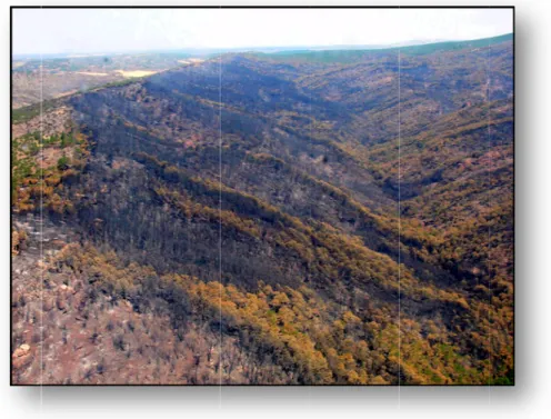
(panoramic and close‐ups) as reference for the post‐processing phase. Figure 3 shows
examples of field plots with diverse CBI values.
Since the field work started only 3 weeks after the fire and due to the risk of dead trees
collapsing, it was difficult to gain access to some parts of the burnt area. Areas with maximum
slopes were not covered, as recommended by Key and Benson (2004) in the specifications of CBI.
Finally, field spectroscopy was carried out in the study area 20 days after the fire using a CROPSCAN multi‐spectral radiometer (CROPSCAN, Inc., 1932 Viola Heights Lane NE Rochester,
MN 55906 USA, http://www.cropscan.com). This radiometer was selected for having the same spectral resolution as the satellite imagery used in this study (Landsat TM). Several types of
burned and unburned vegetation were measured on different backgrounds (charcoal, litter
and ash). The spectra were used as reference for satellite reflectance analysis.
A
B
C
Figure 3. Examples of high (A, CBI=3), moderate (B, CBI=2.35) and low (C, CBI=0.9) burn severity.
2.3. Remotely sensed data
Two Landsat 5 Thematic Mapper (TM) images (path 200, row 32), corresponding to July 1st,
2004 (pre‐fire) and August 5th, 2005 (post‐fire) were selected. The original digital numbers of
reflective TM bands were scaled to radiance values (Lλ) using the procedure proposed by
Chander and Markham (2003) for TM images acquired after May 5th, 2003.
The radiance to reflectance (ρ) conversion (atmospheric correction) was performed using
the dark object method proposed by Chavez (1996) with band‐fixed transmissivity values. A set of Ground Control Points (GCPs) was selected for the geometric correction using a
Landsat ETM+ ortho‐image (from the CORINE 2000 project, UTM 30 T European 1950 mean) as reference. The resulting Root Mean Square Error (RMSE) was under half a pixel (or 15 m). Moreover, pre‐ and post‐fire images were co‐registered (RMSE<15 m).
For the characteristics of the study area, an illumination correction was required. The
correction was carried out using a digital terrain model (DTM, 10 m of resolution) and the
method proposed by Civco (1989). The radiometric fitting between pre‐ and post‐fire images
was tested comparing spectral signatures of the pixels corresponding to areas with low
seasonal changes (asphalt and rock). The comparison of reflectance values returned a
Finally, to cover the entire range of CBI, 47 pixels were selected from the post‐fire image, named PN from 1 to 47, which corresponded to unburned areas (CBI=0, orange points in figure 1), in addition to the 103 field plots.
2.4. Empirical fitting
For the empirical fitting, several spectral indices and transformations were tested. NBR (Key and Benson, 2002; Eq. (2)) was selected for being the only one index specifically developed for burn severity analysis. This index was calculated for the pre‐ and post‐fire images, after which
the ΔNBR (Eq. (3)) was computed. Likewise, NDVI from both pre‐ and post‐fire images was
obtained and consequently, ΔNDVI was generated. In addition to these indices, the Tasselled
Cap (Kauth and Thomas, 1976) transformation and the Hue, Intensity, Saturation (HIS)
transformation (Koutsias et al., 2000) were computed from the TM7, TM4, TM1‐RGB
composition.
Single reflective bands of the TM post‐fire image and the results of spectral indices and linear transformations were correlated against the CBI of all field plots.
Due to the spatial resolution of the TM sensor and to the size of field plots (30‐m diameter), the data to be used in the empirical fittings were extracted using the pixel value corresponding
to the coordinates of the centre of each field plot.
As suggested by Key and Benson (2005), a sub‐sampling was carried out from the total 150 plots to obtain a similar representation of each severity group (CBI under 1.5, from 1.5 to 2.5,
and over 2.5). A total of 46 plots were randomly selected and used for the calibration of the
empirical model. In this sub‐sample, the full range of severity variation is represented. The
remaining 104 plots were used in the validation phase. The linear regression technique applied was the stepwise forward selection (SPSS 13), and the empirical fitting was evaluated using the RMSE between observed and predicted CBI.
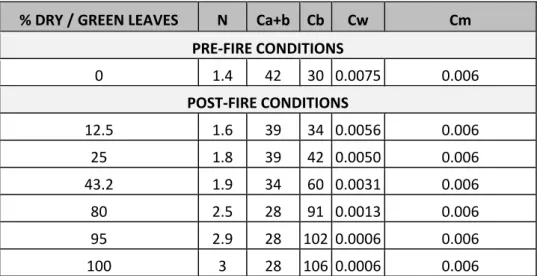
2.5. Simulation models
The simulation model used in this paper was developed by Chuvieco et al. (2006). They used
a leaf canopy model combination based on the PROSPECT and KUUSK RTM, respectively. The
CBI was simulated by changing the substrate conditions (from soil to charcoal), the leaf
0.01). Two vegetation strata, plus the substrate were included in the simulations. Two simulation scenarios were considered: a wide short‐term and a post‐fire high severity. For this
paper, the wide short‐term was selected since it considered general short‐term effects of
recent fires (within a few weeks after fire). To simulate this scenario, the authors assumed that
the CBI of each stratum changed independently from the other two. However, within each
stratum the increase in the percentage of altered foliage (PFA) and in the percentage of
change in leaf cover (PCC) occur simultaneously. All the simulations were run for the solar
spectrum (from 400 to 2500 nm) at 10‐nm intervals (201 spectral bands). The number of the
simulation cases was reduced by fixing the following variables throughout all the simulations:
leaf angle distribution= plagiophile, leaf shape=ellipse form (eccentricity=0.95), sun zenith
angle=30°, nadir angle=0°, azimuth angle=0°.
To avoid unrealistic combinations, three rules were applied:
1. CBI B+C > CBI A: since it is very unlikely that the CBI of a shrub stratum (b1mtall) can be greater than the CBI of the soil.
2. CBI B+C > CBI D+E: eliminates simulations when the CBI of a canopy is greater than the
CBI of the understory, which was never observed in the field plots.
3. CBI B+C <4 *CBI A: eliminates simulations where the CBI of the understory is four times greater than the CBI of the background soil, in agreement with field observations.
Finally, from the original 1000 simulations, only 278 were considered significant and their
corresponding CBI values ranged from 0.45 to 3. To fill the range gap existed between 0 and
0.45 (CBI nominally ranges from 0 to 3), additional simulations of unburned vegetation
conditions were added to the original 278. These two spectral signatures were also derived
from a simulation using the Kuusk model (David Riaño, personal communication).
2.6. Model inversion strategies
Inversion methods use different approaches to compare the simulated and observed
spectra. A first distinction may be made on whether the process computes the simulated
spectra before the actual inversion or does it iteratively during the inversion process. The former is more common, since the computation time is reduced (the iterative process requires running the model for each pixel) and the simulated spectra are better selected according to
realistic assumptions (Gastellu‐Etchegorry et al., 2003; Kimes et al., 2002; Liang, 2004). This
since it provided a more operational approach to CBI retrieval. The LUT was generated from our forward simulations, considering the input scenarios previously commented.
The comparison between observed and simulated spectra can be based on several criteria,
being the most common the minimum quadratic distance and neural networks (Kimes et al.,
2000). In this paper, the minimum angle between the simulated and observed spectra was
used, since it provides a consistent measure of spectral similarity. For this study, all the spectra generated for the look‐up table were used to build a spectral library (in ENVI 4.2™), which was
adapted to simulate the response of TM sensor. Then, all the spectra in the resulting library
were used as endmembers to perform a Spectral Angle Mapper (SAM) supervised classification
of the post‐fire TM image. SAM is a pixel‐based supervised classification technique that
measures the similarity between two spectra, in our case between each pixel in the TM image and the simulated spectra of CBI values included in the LUT. This similarity is computed from
the spectral angle (in radians), when each spectrum is considered as an m‐dimensional feature
vector, with m being the number of spectral channels (Debba et al., 2005; Kruse et al., 1993).
This angle is independent of the length of vectors (Bakker and Schmidt, 2002), so it is
insensitive to illumination or albedo effects.
To be able to compare the results from the model inversion to the results from empirical
estimation, the spectral angle threshold of SAM classification was left open. In this way, the
not‐classified category was not present.
After applying the SAM algorithm, a CBI value was assigned to each pixel in the image, the result of which can be directly considered as a burn severity map.
Finally, the verification was performed extracting the values of pixels corresponding to the same plots as in the empirical validation and by computing the RMSE between modelled and observed CBI.
3.
Results
3.1. Results of the field work
Most of the burned area presented very high observed CBI values. Only 28 of 103 field plots
have CBI values lower than 2.5, and 32 have CBI higher than 2.9. In all cases the burn severity is higher in the understory than the overstory.
3.2. Empirical fitting between spectral indices and CBI values
Table 1 shows the correlations between the CBI of the total plot and a number of variables:
reflective bands of the post‐fire TM image, spectral indices and results from linear
transformation.
The CBI of the total plot correlated most strongly with Greenness (Tasselled Cap
transformation result) and ΔNDVI (r=−0.76 and r=0.76, respectively), followed by TM band 4
and NDVI (r=−0.75). NBR and ΔNBR had a correlation coefficient slightly lower (r=−0.72 and
r=0.73, respectively). These results suggest that the NIR is the most sensitive spectral region
for burn severity estimation. In contrast, the SWIR has a low sensitivity to minor differences in
high CBI values. This explains why TM band 7 (SWIR) had a low correlation (r=0.39), due to the fact that most observed CBI values were high.
Table 1. Correlation (r of Pearson) between the CBI of the total plot and the following variables: spectral bands (TM1 to TM7of post‐fire image), spectral indices (NDVI, dNDVI, NBR and dNBR) and linear transformation results (Albedo, Greenness and Moisture= results from Tasselled Cap transformation; H, I and S= results from Hue, Intensity and Saturation transformation) of TM images. In bold are significant (p< 0.05) values.
r Pearson correlation coefficients CBI of the total plot TM1 (0.45 ‐0.52 μm) 0.07
TM2 (0.52 ‐0.60 μm) ‐0.19 TM3 (0.63 ‐0.69 μm) ‐0.06 TM4 (0.76 ‐0.90 μm) ‐0.75 TM5 (1.55 ‐1.75 μm) 0.05 TM7 (2.08 ‐2.35 μm) 0.39
NBR ‐0.72
dNBR 0.73
NDVI ‐0.75
dNDVI 0.76
I ‐0.30
H 0.33
S ‐0.68
Albedo ‐0.31
Greenness ‐0.76
Moisture ‐0.54
A total of 46 randomly sub‐sampled plots were used to perform the linear regression.
Although only small number of unburned plots were also included, their relative weight in
the final linear fitting could be very significant. To avoid this, the coefficient D by CooK (SPSS) was computed to test the influence of each CBI value used in the calibration of regression
model (Peña Sánchez de Rivera, 1989). This analysis confirmed that all selected values of CBI
were acceptable (p<0.05).
The linear regression returned a model with the ΔNDVI and the S result of the HIS
transformation:
1.679 2.83∆ 9.574
This model explained 67% of the total variance and its fitting showed an R2adjusted =0.66 (Table 2).
Table 2. Empirical fitting and model inversion performances.
EMPIRICAL FITTING MODEL INVERSION
REGRESSION VALIDATION VALIDATION
R2 R2adj. R2 RMSE R2 RMSE
0.82 0.66 0.85 0.64 0.84 0.48
In the verification phase, Eq. (4) was applied to the remaining 104 plots. The correlation
obtained was r2 =0.85 (figure 4)and the RMSE between estimated and observed CBI was 0.64
(Table 2). However, there is a marked offset from the 1:1 linear fitting, due to the
overestimation of unburned plots.
Figure 4. Scatter plot between estimated and observed CBI.
The unburned plots (CBI=0) were generally overestimated (figure 5), because this severity
level did not clearly correspond to a single value of estimators (ΔNDVI and S). According to the composition of each plot, intermediate CBI values (0.9 < CBI <2.7) were either:
9 underestimated when the fraction of cover (FCOV) of the tree strata was high, and
over 50% of the scorched leaves remained on the tree crowns (plots 5, 11, 27, 58
and 62, figures 5 and 6A). In such cases the estimated CBI was more similar to the
observed CBI of the overstory.
9 Overestimated when the FCOV of the overstory was under 10% and the observed
CBI of the understory was high (plots 44, 47 and 54, figures 5 and 6B).
High burn severity levels (CBI>2.7) were underestimated although there does not seem to
be a clear relationship with the composition these plots.
y = 0.6244x + 0.5901 R2 = 0.85 RMSE=0.64
0.0 0.5 1.0 1.5 2.0 2.5 3.0
0.0 0.5 1.0 1.5 2.0 2.5 3.0
CBI observed
C
B
I es
ti
m
a
te