Monterrey, Nuevo León a 2 de Junio de 2003
Lic. Arturo Azuara Flores:
Director de Asesoria Legal del Sistema
Por medio de la presente hago constar que soy autor y titular de la obra
titulada: Evaluating Organization and Conectivity in Ad-Hoc Wireless Networks
", en los sucesivo LA OBRA, en virtud de lo cual autorizo a el Instituto Tecnológico y de Estudios Superiores de Monterrey (EL INSTITUTO) para que efectue la divulgación, publicación, comunicación publica, distribución y reproducción, asi como la digitalización de la misma, con fines académicos o propios al objeto de EL INSTITUTO.
El Instituto se compromete a respetar en todo momento mi autoría y a otorgarme el crédito correspondiente en todas las actividades mencionadas anteriormente de la obra.
De la misma manera, desligo de toda la responsabilidad a EL INSTITUTO por cualquier violación a los derechos de autor y propiedad intelecutal que cometa el suscrito frente a terceros.
Evaluating Organization and Connectivity in Ad-Hoc Wireless
Networks-Edición Única
Title Evaluating Organization and Connectivity in Ad-Hoc
Wireless Networks-Edición Única
Authors Aldo López Gudini
Affiliation ITESM
Issue Date 2003-06-01
Item type Tesis
Rights Open Access
Downloaded 18-Jan-2017 23:00:25
Monterrey
Campus Monterrey
Divisi´
on de Electr´
onica, Computaci´
on, Informaci´
on, y
Comunicaciones
Programa de Graduados
Evaluating Organization and Connectivity in Ad-Hoc Wireless
Networks
THESIS
Presented as a partial fulfillment of the requeriments for the degree of
Master of Science in Electronic Engineering
Major in Telecommunications
Aldo L´
opez Gudini
Monterrey
Campus Monterrey
Divisi´
on de Electr´
onica, Computaci´
on, Informaci´
on, y
Comunicaciones
Programa de Graduados
The members of the thesis committee recommended the acceptance of the thesis of Aldo L´opez Gudini as a partial fulfillment of the requeriments for the degree of Master of
Science in:
Electronic Engineering
Major in Telecommunications
THESIS COMMITTEE
C´esar Vargas Rosales, Ph.D.
Advisor
Jorge Carlos Mex Perera, Ph.D.
Synodal
Artemio Aguilar Couti˜no, M.Sc.
Synodal
Approved
David Garza Salazar, Ph.D.
Director of the Graduate Program
To my parents Maria del Pilar and Genaro Noe, for their unconditional support in all my life. To my brother Miguel Angel for support to me at any moment.
I am very grateful to my thesis advisor C´esar Vargas Rosales Ph.D. for all these time in which we works together, for all his professional advice for the accomplishment of this work and for his friendship. Because, without his guidance this thesis would not have been possible. Sincerely thanks Doc. Also I want to thank to Jorge Carlos Mex Perera, Ph.D. and Artemio Aguilar Couti˜no, M.Sc. for their valuable comments for the enhancement of this work.
To the ITESM and CONACYT for give me the oportunity of realize my graduate studies.
I want to thank too all my friends of CET, specially to Lluvia, Anabel, Martha, Dulce, Rodolfo, Oscar, Edson, Abraham, Luis, Ulises, Marco, Rafael, Fernando, Alejandro Trigos, and Rene. To all my friends of the 4th floor; Michelle, Vladimir, Max, Sergio and Roger.
Aldo L´
opez Gudini
Networks
Aldo L´opez Gudini, M.Sc.
Instituto Tecnol´ogico y de Estudios Superiores de Monterrey, 2003
Los sistemas inal´ambricos han experimentado un r´apido crecimiento, donde el principal objetivo de este crecimiento es la de alcanzar la satisfacci´on del cliente, y de esta forma lograr que los usuarios puedan comunicarse sin la necesidad de una conexi´on convencional (alambrica). Las redes inal´ambricas ad hoc est´an constituidas por nodos m´oviles conecta-dos entres si por multienlaces de comunicaci´on. Esta red inal´ambrica a diferencia de las dem´as redes no tiene una estructura convencional como las redes inal´ambricas tradicionales, las cuales presentan una estructura predefinida y adem´as fija, de aqu´ı el surgimiento de problemas de este tipo de redes con relaci´on al ruteo y el mantenimiento punto a punto de un enlace dadas las circunstancias de movilidad que cada nodo presenta.
Otro problema relacionado con la poca cantidad de nodos es la conectividad, la cual es baja si existe una baja cantidad de nodos, pero esta de igual forma puede ser baja si los nodos est´an organizados en diferentes grupos.
List of Figures iii
List of Tables vii
Chapter 1 Introduction 1
1.1 Objective . . . 2
1.2 Justification . . . 2
1.3 Contribution . . . 2
1.4 Organization . . . 2
Chapter 2 Background 3 2.1 Ad Hoc Wireless Networks . . . 3
2.2 Types of Ad Hoc Mobile Communications . . . 4
2.2.1 Movements by Nodes in a Route . . . 4
2.2.2 Movements by Subnet-Bridging Nodes . . . 5
2.3 Ad Hoc Routing Protocols . . . 6
2.3.1 Table-Driven Approaches. . . 6
2.3.2 Source-Initiated On-Demand Approaches . . . 10
2.4 Clustering . . . 21
2.4.1 Cluster Based Routing Protocol (CBRP) . . . 21
2.4.2 Access-Based Clustering Protocol (ABCP) . . . 29
2.5 Connectivity . . . 33
Chapter 3 Model Description 35 3.1 Point Processes . . . 35
3.2 Virtual Cluster-based Routing Protocol (VCRP) . . . 36
3.2.1 Considerations to Group N-nodes within Virtual Clusters. . . 37
3.2.2 Connection between Two Nodes in a Two-Hop Trajectory. . . 37
3.3 Algorithm for Membership Allocation in a Virtual Cluster . . . 38
3.3.1 Clustering By Distance . . . 39
3.3.2 Clustering By Power . . . 40
3.4 Log-normal Shadowing . . . 40
3.5 Generation of Mobility and Packets . . . 40
3.6 Types of Connectivity . . . 42
3.6.1 Absolute Connectivity of Each Node. . . 43
3.6.2 Network Connectivity toh-hops . . . 44
3.6.3 Average Connectivity of each Node to h-hops in time. . . 45
3.6.4 Total Absolute Connectivity of the Network by Power . . . 45
3.6.5 Total Absolute Connectivity of each Node by Power in time . . . . 46
3.7 Virtual Cluster Fragility . . . 46
Chapter 4 Numerical Results 51 4.1 Simulation . . . 51
4.1.1 General Scenario . . . 53
4.1.2 Nodes Population Scenarios . . . 53
4.2 Analyzing Node Connectivity . . . 57
4.3 Analyzing Network Connectivity to h-hops . . . 64
4.4 Analyzing Total Absolute Connectivity of the Network . . . 64
4.5 Analyzing Fragility . . . 72
Chapter 5 Conclusions 79 5.1 General Conclusions . . . 79
5.2 Future Work . . . 80
Bibliography 81
2.1 Mobile Host Network . . . 4
2.2 Mobile ad hoc subnets merging and fragmenting . . . 5
2.3 Categorization of ad hoc protocols . . . 7
2.4 A CSGR path is constrained to cluster heads. . . 9
2.5 AODV route discovery. . . 11
2.6 (a) Route creation, and (b) route maintenance in TORA . . . 14
2.7 (a) Concepts LAR, and (b) route physical distance. . . 16
2.8 The ZRP Architecture. . . 17
2.9 The proactive Intrazone Routing Protocol (IARP) . . . 18
2.10 Hybrid Approach - Zone routing protocol. . . 19
2.11 The reactive Interzone Routing Protocol (IERP) . . . 20
2.12 Link/Connection Status Sensing Mechanism . . . 25
2.13 Transition diagram of a node in CBRP . . . 27
2.14 Adjacent Cluster Discovery . . . 28
2.15 Format of control of channel in the Cluster of ad hoc network . . . 31
2.16 State transition diagram of a node in ABCP . . . 32
2.17 h-Connectivity . . . 33
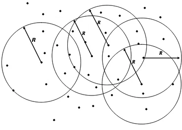
3.1 N-nodes with Poisson distribution . . . 36
3.2 Virtual clusters formation of size R. . . 37
3.3 Two hops connection . . . 38
3.4 Clustering using ZRP and VCRP . . . 39
3.5 Nodes mobility in ad hoc network . . . 41
3.6 Node Mobility from its starting point . . . 42
3.7 Shift of position of a node in a Ad hoc network . . . 43
3.8 Algorithm evaluation of the ad hoc network . . . 47
3.9 Virtual Cluster Fragility, with low fragility . . . 48
3.10 Virtual Cluster Fragility, with high fragility . . . 49
4.1 Closed coverage area . . . 52
4.2 Initial scenario with 25 nodes and link dij ≤R . . . 53
4.3 Initial scenario with 25 nodes and link Pthreshold≤PRx . . . 54
4.4 Initial scenario with 50 nodes and link dij≤R . . . 55
4.5 Initial scenario with 50 nodes and link Pthreshold≤PRx . . . 56
4.6 Initial scenario with 100 nodes and linkdij≤R . . . 56
4.7 Initial scenario with 100 nodes and linkPthreshold≤PRx . . . 57
4.8 Final scenario with 25 nodes and linkdij≤R . . . 58
4.9 Final scenario with 25 nodes and linkPthreshold≤PRx. . . 58
4.10 Final scenario with 50 nodes and link dij≤R . . . 59
4.11 Final scenario with 50 nodes and link Pthreshold≤PRx. . . 59
4.12 Final scenario with 100 nodes and link dij≤R . . . 60
4.13 Final scenario with 100 nodes and link Pthreshold≤PRx . . . 60
4.14 Average Connectivity with Ntot = 25 and linkdij≤R . . . 61
4.15 Average Connectivity with Ntot = 25 and linkPthreshold≤PRx . . . 61
4.16 Average Connectivity with Ntot = 50 and linkdij≤R . . . 62
4.17 Average Connectivity with Ntot = 50 and link Pthreshold ≤PRx . . . 63
4.18 Average Connectivity with Ntot = 100 and linkdij≤R . . . 63
4.19 Average Connectivity with Ntot = 100 and link Pthreshold≤PRx . . . 64
4.20 Network Connectivity to 1-hop and link dij≤R . . . 65
4.21 Network Connectivity to 1-hop and link Pthreshold≤PRx . . . 65
4.22 Network Connectivity to 2-hop and link dij≤R . . . 66
4.23 Network Connectivity to 2-hop and link Pthreshold≤PRx . . . 66
4.24 Network Connectivity to 3-hop and link dij≤R . . . 67
4.25 Network Connectivity to 3-hop and link Pthreshold≤PRx . . . 67
4.26 Network Connectivity to 4-hop and link dij≤R . . . 68
4.27 Network Connectivity to 4-hop and link Pthreshold≤PRx . . . 68
4.28 Total Absolute Connectivity considering dij≤R . . . 69
4.29 Total Absolute Connectivity considering Pthreshold ≤PRx . . . 70
4.30 Empirical CDF of the Total Absolute Connectivity considering R . . . 70
4.31 Empirical CDF of the Total Absolute Connectivity considering PRx . . . . 71
4.32 Histograms normalized of the Total Absolute Connectivity considering R . 71 4.33 Histograms normalized of the Total Absolute Connectivity considering PRx 72 4.34 Total Absolute Connectivity samples with Ntot=25 vs Gaussian pdf . . . . 73
4.35 Total Absolute Connectivity samples with Ntot=50 vs Gaussian pdf . . . . 73
4.36 Total Absolute Connectivity samples with Ntot=100 vs Gaussian pdf . . . . 74
4.37 Fragility with Ntot=25 considering dij ≤R . . . 75
4.38 Fragility with Ntot=25 considering Pthreshold ≤PRx . . . 75
4.40 Fragility with Ntot=50 considering Pthreshold≤PRx . . . 76
4.41 Fragility with Ntot=100 considering dij ≤R . . . 77
4.1 Node Parameters of Simulation . . . 52
4.2 Network Traffic Parameters . . . 52
4.3 Environment Scenario Specifications . . . 54
4.4 Average of Connectivity . . . 63
4.5 Average of Fragility . . . 75
Introduction
The ad hoc wireless network consists of mobile nodes connected by links called multilinks of communication. This wireless network does not have a conventional structure as tradi-tional wireless networks do, which present a predefined structure and fixed, the problems start here and they are related to routing, the maintenance of the point to point link, the bandwidth among which they directly affect the QoS of the ad hoc network degrading it, [1], [2].
Due to the benefits and to the unique versatility that present the ad hoc networks in certain environments and applications being implemented; the interest in the development of this type of network in special, has come to more; in the military areas, rescue, in zones of hostile natural and environment disasters. One of the main problems that appear in ad hoc networks is the updating of the topology, since the nodes have mobility and therefore the structure of the network varies with time; because nodes are added or eliminated ran-domly and such process takes us to an update in the topology for each case; the variability of the network can be so frequent that the update cannot be propagated to all the network by broadcasting messages, which consist of directions and alternative routes, or some other method of update like flooding. In other words knowing the positions the neighboring nodes to the node source so that at certain moment can be used to create a trajectory towards the destination node that would guarantee an acceptable QoS to us, [1], otherwise, if it were not gotten to possible alternative routes and the link failed in the central part, that is, when another node takes part in the trajectory between the node source and the destination, the connection would be lost and as consequence the QoS is also degraded in the ad hoc network, [3].
The study of the mobility of these nodes within the ad hoc network can be made dividing the area or space in cluster called cells where the network ad hoc is implemented for analysis and management of an easy way.
1.1
Objective
The objective of this thesis is to evaluate the performance of ad hoc networks with respect to the organization, connectivity and mobility of the nodes, using point processes to study of it.
1.2
Justification
The ad hoc networks are systems of fast implementation that do not count on permanent physical infrastructure. Due to this, to obtain the interconnections of nodes source and destination, it is necessary to establish topologies on which the routes are constructed that will transport the information, but given the ample class of stations (fixed, semi-portable, mobiles), is necessary to study the way in which the nodes will be organized to be able to define a topology, which will work the network and the necessary connectivity for its operation and their formation and its maintenance.
1.3
Contribution
We propose new parameters with the goal of analyzing the organization, connectivity and mobility of ad hoc wireless networks with different density of node.
1.4
Organization
Background
Wireless systems have experienced a fast growth where their main objective is to look for customer´s satisfaction, so the users can be in communication without the necessity of a wired connection.
In the present Chapter we analyze briefly what an ad hoc wireless network is, its routing protocols and its self-organization for a best management.
2.1
Ad Hoc Wireless Networks
An ad hoc wireless network is a collection of two or more devices equipped with wireless communications and networking capability. Such devices can communicate with another node that is immediately within their radio range or one that is outside their range.
An ad hoc wireless network is self-organizing and adaptive. This means that a formed network can be de-formed on-the-fly without the need for any system management. The term “ad hoc” tends to imply “can take different forms” and can be mobile, standalone, or networked, [4], [6].
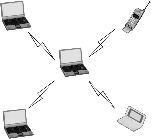
Since ad hoc wireless devices can take different forms (for example, palmtop, laptop, internet mobile phone, etc.), as show in Figure 2.1, the computation storage, and commu-nications capabilities of such devices will vary tremendously. Ad hoc devices should not only detect the presence of connectivity with neighboring devices/nodes, but also identify what type the devices are and their corresponding attributes. There is no need for any fixed radio base stations, no wires or fixed route, [1], [2], [6]. Due the mobility, routing information will have to change to reflect changes in link connectivity.
Ad hoc wireless communications can occurs in several different forms. For a pair of
ad hoc wireless nodes, communications will occur between them over period of time until the session is finished or one of the nodes has moved away. This resembles a peer-to-peer communication scenario.
Figure 2.1: Mobile Host Network
Another form occurs when two or more devices are communicating among themselves and they are migrating in groups. The traffic pattern is, therefore, one where communica-tions occur over a longer period of time. This resembles the scenario of remote-to-remote communication, [6].
Finally, we can have a scenario where devices communicate in a non-coherent fashion and their communication sessions are, therefore, short, abrupt, and undeterministic.
2.2
Types of Ad Hoc Mobile Communications
Mobile host in an ad hoc mobile network can communicate with their immediate peers, that is, peer-to-peer, that are in a single radio hop away. However, if three or more nodes are within range of each other (but no necessarily a single hop away from one another), then remote-to-remote mobile node communications exist.
This section examines the types of mobile host movements that can affect validity of routes directly.
2.2.1
Movements by Nodes in a Route
An SRC node in a route has a downstream link, and when it moves out of its downstream neighbor’s radio coverage range the existing route will immediately become invalid.
Likewise, when a DEST node moves out of the radio coverage of its upstream neigh-bor, the route becomes invalid. However, unlike the earlier case, here, the upstream nodes will have to be informed so they can erase their invalid route entries, [6].
All these movements cause many conventional distributed routing protocols to respond in sympathy with the link changes. This results in an updating of all the remaining nodes within the network. The updating process involves broadcasting over the wireless medium, which results in wasteful bandwidth and an increase in the overall network control traffic. Hence new routing protocols are needed, [3], [6].
2.2.2
Movements by Subnet-Bridging Nodes
In addition to the above-mentioned mobility scenario, any movement by a node that is performing a subnet-bridging function between two mobile subnets can fragment the mobile subnet into smaller subnets. The property of a mobile subnet states that if both the SRC and DEST nodes are elements of the subnet, a route or routes should exist unless the subnet is partitioned by some subnet-bridging mobile nodes.(See Figure 2.2).
Subnet (S1) Subnet (S2)
Merged Subnet
Subnet (S1) Subnet (S2)
Merged Subnet
2.3
Ad Hoc Routing Protocols
One of the major challenges in designing a routing protocol for the ad hoc networks stems from the fact that, on one hand, to determine a packet route, a node needs to know at least the reachability information to its neighbors. On the other hand, in an ad hoc network, the network topology can change quite often. Furthermore, as the number of network nodes can be large, the potential number of destinations is also large, requiring large and frequent exchange of data (e.g., routes, routes updates, or routing tables) among the network nodes. Thus, the amount of update traffic can be quite high. This is in contradiction with the fact that all updates in a wirelessly interconnected ad hoc network travel over the air and, thus, are costly in resources.
The presence of mobility implies that links make and break often in an indetermin-istic fashion. Note that the classical distributed Bellman-Ford routing algorithm is used to maintain and update routing information in a packet radio network. While distance-vector-based routing is not designed for wireless network, it is still applicable to packet radio networks since the rate of mobility is not high. Hence, ad hoc mobile networks are different from radio networks since nodes can move more freely, resulting in a dynamically changing topology. Existing distance-vector and link-state-based routing protocols are un-able to catch up with such frequent link changes in ad hoc wireless networks, resulting in poor route convergence and very low communication throughput. Hence, new routing protocols are needed.
Since the advent of the DARPA packet radio network in the early 1970s, numerous protocols have been developed for ad hoc mobile networks, such protocols must fight with their own limitations of its network, which include high power consumption, low bandwidth, and high error rate, [3], [6], [15]. The routing protocols may generally be categorized as (Figure 2.3):
• Table-driven
• Source initiated on-demand-driven
2.3.1
Table-Driven Approaches.
AD HOC ROUTING PROTOCOLS
TABLE DRIVEN
SOURCE-INITIATED ON DEMAND
DSDV
CGSR
AODV DSR LMR
TORA
ABR
SSR WRP
HYBRID
ZRP
AD HOC ROUTING PROTOCOLS
TABLE DRIVEN
SOURCE-INITIATED ON DEMAND
DSDV
CGSR
AODV DSR LMR
TORA
ABR
SSR WRP
HYBRID
ZRP
Figure 2.3: Categorization of ad hoc protocols
topology by propagating route updates throughout the network to maintain the consistent from, [3], [6].
Destination Sequenced Distance Vector (DSDV)
Destination Sequenced Distance Vector (DSDV) routing is a table-driven routing protocol based on the classical distributed Bellman-Ford routing algorithm. The improvement made here is the avoidance of routing loops in a mobile network of routers. Each node in the mobile network maintains a routing table in which all of possible destinations within the non-partitioned network and the number of routing hops (in this case, number of radio hops) to each destination are recorded.
A sequence numbering system is used to allow mobile hosts to distinguish state routes from new ones. Routing tables updates are sent periodically throughout the network to maintain table consistency; as a result we generate a lot of control traffic in the network, rendering an inefficient utilization of network resource. DSDV with the aim of alleviate this problem uses two types of route update packets; the called full dump; this type of packet carries all available routing information and require multiple network protocol data units (NPDUs). During periods of occasional movement, these packets are transmitted infrequently. Smaller incremental packets are used to relay only information that has changed since that last full dump, [3], [19], [16].
Wireless Routing Protocol (WRP)
wireless network. It avoids the count-to-infinity problem by forcing each node to perform consistency checks of predecessor information reported by all its neighbors. This ultimately eliminates looping situations and provide faster route convergence when a link failure event occurs.
In WRP, nodes learn about the existence of their neighbors from the receipt of ac-knowledgments and other messages. If a node is not sending packets, it must send a HELLO message within a specified time period to ensure that information connectivity is properly reflected. When a mobile receive a HELLO massage from a new node, the new node trans-mits a copy of its routing table information.
WRP must maintain four tables, namely:
• Distance table • Routing table • Link-cost table
• Message retransmission list (MRL) table.
The distance table indicates the number of hop between a node and its destination. The routing table indicates the next-hop node. The link-cost tale reflects the delay associ-ated with particular link. The MRL contains the sequence number of the update message, a retransmission counter, an acknowledgment required flag vector, and a list of the updates sent in the update message.
To ensure that routing information is accurate, mobiles send update messages period-ically to their neighbors. The updated message contains a list of changes (the destination, the distance to destination, the predecessor of the destination), as well as a list of responses indicating which mobile should acknowledge the update, [20], [21].
Cluster Switch Gateway Routing (CSGR)
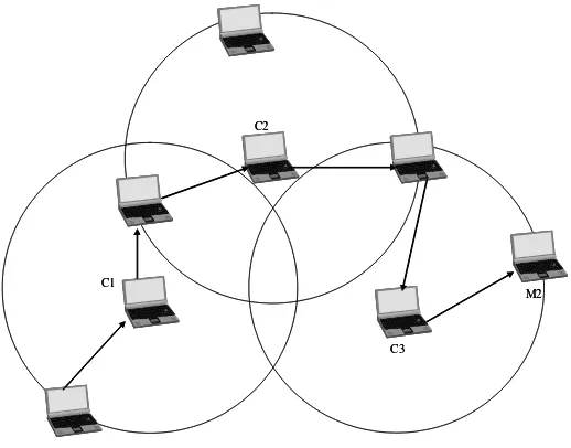
Although using a cluster head allows some form of control and coordination. When a cluster head moves away, another new cluster head must be selected. This can be prob-lematic if a cluster head changing frequently and nodes will be spending a lot of time converging to a cluster head instead of forwarding data toward their intended destinations. To avoid invoking cluster head reselection every time the cluster membership changes, a least cluster changes (LCC) algorithm is introduced. The LCC algorithm, cluster head only change when two cluster head come into contact, or when a node moves out of all other heads.
CSGR uses DSDV as the underlying routing scheme. However, it modifies DSDV by using hierarchical cluster-head-to-gateway routing. Gateway nodes are nodes that are within communication range of two or more cluster heads. As show in Figure 2.4, a packet sent by a node is first routed to its cluster head, and then the packet is routed from a cluster head to a gateway to another cluster head, and so on until the cluster head of the destination node is reached.
C1
C2
C3
M2 C1
C2
C3
[image:23.612.187.446.394.597.2]M2
Figure 2.4: A CSGR path is constrained to cluster heads.
2.3.2
Source-Initiated On-Demand Approaches
An approach that is different from table-driven routing is source-initiated on-demand rout-ing. This type of routing creates routes only when desired by the source node. When a node requires a route to a destination, it initiates a route discovery process within the network. This process is completed once a route is found or all possible route permutations have been examined, [6].
Ad Hoc On-Demand Distance Vector Routing (AODV)
The Ad Hoc On-Demand Distance Vector Routing (AODV) routing protocol builds on the DSDV algorithm previously described. AODV is an improvement on DSDV because it typically minimizes the number of required broadcasts by creating routes on an on-demand basis, as opposed to maintaining a complete list of route as in the DSDV algorithm. This protocol is classified as a pure on-demand route acquisition system.
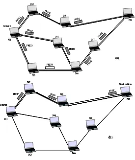
When a source node wants to send a message to some destination node and does no already have a valid route to that destination, it initiates a path discovery process to locate the other node. It broadcasts a route request (PREQ) packet to its neighbors, which then forward the request to their neighbors, and so on, until either the destination or an inter-mediate node with a “fresh enough” route to the destination is located (Figure 2.5). AODV uses destination sequence members to ensure that all routes are loop-free and contain the most recent route information.
During the process of forwarding the PREQ, intermediate nodes record in their route tables the addresses of neighbors from which the first copy of the broadcast packet was received, thereby establishing a reverse path. If additional copies of the same PREQ are later received, these packets are silently discarded. Once the PREQ has reached the desti-nation or an intermediate node with a “fresh enough” route, the destidesti-nation/intermediate node responds by unicasting a route reply (PREP) packet back to the neighbor from which it first received the PREQ (Figure 2.5).
Source N1 N2 N5 N8 N4 N3 N7 N6 (a) PREQ PREQ PREQ PREQ PREQ PREQ PREQ PR EQ PREQ Source N1 N2 N5 N8 N4 N3 N7 N6 (a) PREQ PREQ PREQ PREQ PREQ PREQ PREQ PR EQ PREQ Source Destination N1 N2 N5 N8 N4 N3 N7 N6 (b) PREP PREP PREP Source Destination N1 N2 N5 N8 N4 N3 N7 N6 (b) Source Destination N1 N2 N5 N8 N4 N3 N7 N6 Source Destination N1 N2 N5 N8 N4 N3 N7 N6 (b) PREP PREP PREP
route is still desired.
An additional aspect of the protocol is the use of HELLO message which are periodic local broadcast made by node to inform each mobile node of other nodes in its neighbor-hood. HELLO messages can be used to maintain the local connectivity of a node. However, the use of HELLO message is not required. Nodes listen for retransmissions of data packet to ensure that the next hop is still within reach, [3], [15], [16], [23].
Dynamic Source Routing (DSR)
Dynamic Source Routing (DSR), is an on-demand routing protocol that is based on the concept of source routing. Mobile nodes are required to maintain route caches that contain the source routes of which the mobile is aware. Entries in the route cache are continually updated as new route are learned.
The protocol consists of two major phases:
• Route discovery • Route maintenance
When a mobile node has a packet to send to some destination, it first consults its route cache to determine whether it already has a route to the destination. If it has an unexpired route to the destination, it will use this route to send the packet. On the other hand, if the node does not have such a route, it initiates route discovery by broadcasting a route request packet. This route request message contains the address of the destination, along with the source node’s address and a unique identification number. Each node re-ceiving the packet checks whether it knows of a route to the destination. If it does not, it adds its own address to the route record of the packet and then forwards the packet along its outgoing links. To limit the number of route request propagated on the outgoing links of a node, a mobile only forwards the route request if the request has not yet been seen by the mobile and if the mobile’s address has not already appeared in the route record. A route reply is generated when either the route request reaches the destination itself, or when it reaches an intermediate node that contains in its route cache an expired route to the destination.
truncated. When a route error packet is received, the hop in error is removed from the node’s route and all routes containing the hop are truncated at that point, [3], [24].
Temporally Ordered Routing Algorithm (TORA)
TORA is high adaptive, loop-free, distributed routing algorithm based on the concept of link reverse. TORA is proposed to operate in a highly dynamic mobile networking environ-ment. It is source-initiated and provides multiple routes for any desired source/destination pair. The key design concept of TORA is the localization of control messages to a very small set of nodes near the occurrence of a topological change (1-hop), [3]. The protocol performs tree basic functions:
• Route creation • Route maintenance • Route erasure.
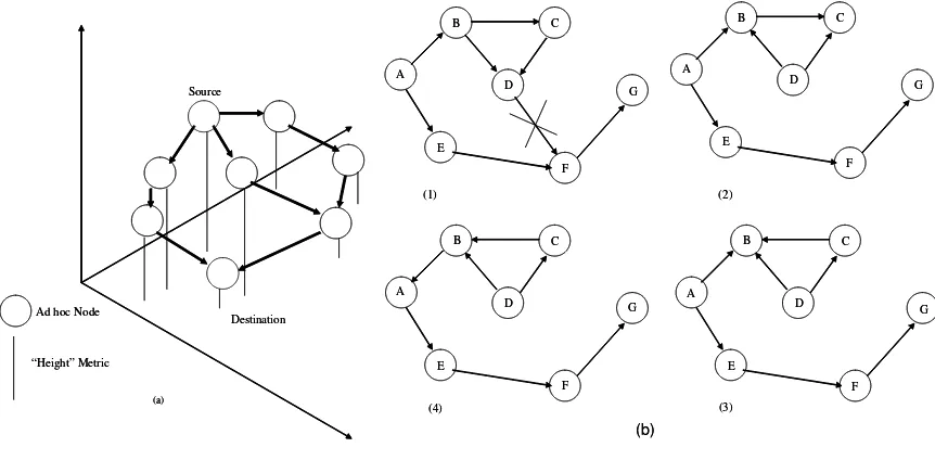
During the route creation and maintenance phases, nodes use a “height” metric to establish a DAG (directed acyclic graph) rooted at the same destination.
Timing is an important factor for TORA because the “height” metric is dependent on the logical time of a link failure; TORA assumes all nodes have synchronized clocks (accomplished via an external time source such as the global positioning system (GPS)). Hence, it is unclear if TORA would function properly in an environment where GPS is not available or is not reliable.
TORA’s metric is a quintuple comprising five elements, namely:
• Logical time link failure
• The unique ID of the node that defined the new reference level • A reflection indicator bit
• A propagation ordering parameter • The unique ID of the node
the network to erase invalid routes, [25].
In TORA, there is a potential for oscillations to occur, especially when multiple sets of coordinating nodes are concurrently detecting partitions, erasing routes, and building new routes based on each other. Because TORA uses internodal coordination, its instability problem is similar to the “count-to-infinity” problem in distance-vector routing protocols, except that such oscillations are temporary and route convergence will ultimately occur, [25].(See Figure 2.6).
Source
Destination Ad hoc Node
“Height” Metric
(a)
Source
Destination Ad hoc Node
[image:28.612.82.513.272.484.2]“Height” Metric (a) A B E F D C G E F D C G E F D C G E F D C G (1) (2) (4) (3) (b) A A A B B B A B E F D C G E F D C G E F D C G E F D C G (1) (2) (4) (3) (b) A A A B B B
Figure 2.6: (a) Route creation, and (b) route maintenance in TORA
Signal Stability Routing (SSR)
Another on-demand protocol is the Signal Stability-Based Adaptive Routing (SSR) proto-col. SSR is a descendent of Associativity-Based Routing (ABR), and ABR predates SSR. Similar to ABR, SSR selects routes based on the signal strength between nodes and a node’s location stability. SSR route selection criteria has a effect of choosing routes that have “stronger” connectivities. SSR can be divided into two cooperative protocols, [3], [26]:
• The Dynamic Routing Protocol (DRP) • The Static Routing Protocol (SRP)
obtained by periodic beacons from the link layer of each neighboring node. After updating all appropriate table entries, the DRP passes a received packet to the SRP.
The SRP processes packets by passing them up the stack if they are the intended receivers, or looking up their destination in the RT and then forwarding them if they are not. If not entry is found in the RT for the destination, a route-search process is initiated to find a route.
The assumption made in SSR is that route search packets arriving at the destination might have chosen the path of strongest signal stability, as the packets are dropped at a node if they have arrived over a weak channel.
When a failed link is detected within the network, intermediate nodes will send an error message to the source indicating which channel has failed. The source initiates another route process to find a new path to the destination. Thereafter, the source sends an erase message to notify all nodes of the broken link, [26].
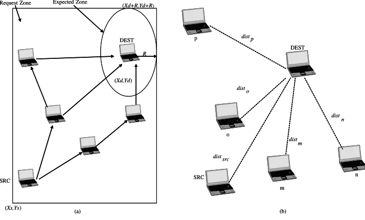
Location-Aided Routing (LAR)
Compared to other ad hoc routing schemes, LAR utilizes location information (via, say, the GPS) to improve the performance of ah doc wireless networks.
LAR limits the search for a new route to smaller request zone, thereby resulting in reduced signaling traffic. LAR defines two concepts:
• Expected zone • Request zone
LAR makes several assumptions. First, it assumes that the sender has advanced knowledge of the destination location and velocity. Based on the location and velocity, the expected zone can be defined. The request zone, however, is the smallest rectangle that includes the location of the sender and expected zone, [6]. (see Figure 2.7).
Zone Routing Protocol (ZRP)
(Xs,Ys) SRC
(Xd,Yd)
R
DEST (Xd+R,Yd+R)
Expected Zone Request Zone
(a) (Xs,Ys)
SRC
(Xd,Yd)
R
DEST (Xd+R,Yd+R)
Expected Zone Request Zone
(a)
dist p
dist o
distsrc
dist m
dist n
p
o
SRC
m
n DEST
(b)
dist p
dist o
distsrc
dist m
dist n
p
o
SRC
m
n DEST
[image:30.612.106.463.138.353.2](b)
Figure 2.7: (a) Concepts LAR, and (b) route physical distance.
zone can, therefore, affect ad hoc communication performance, [4], [27].
In ZRP, a routing zone comprises a few mobile ad hoc nodes within one, two or more hops away from where the central node is formed. Within this zone, a table-driven-based routing protocol is used. A related issue is that of updates in the network topology. For a routing protocol to be efficient, changes in the network topology should have only a local effect. In other words, creation of a new link at one end of the network is an important local event but, most probably, not a significant piece of information at the other end of the network. Globally proactive protocols tend to distribute such topological changes widely in the network, incurring large costs. The ZRP limits propagation of such information to the neighborhood of the change only, thus limiting the cost of topological updates.
ZRP itself has three sub-protocols, see Figure 2.8:
• The proactive (table-driven) Intrazone Routing Protocol (IARP) • The reactive Interzone Routing Protocol (IERP)
• The Bordercast Resolution Protocol (BRP).
NDM IARP IERP
BRP
ICMP
IP
ZRP
A B Exchange of packets between protocols A & B A B Information passed from protocol A to p rotocol B Existing Protocols:
IP Internet Protocol
ICMP Internet Control Message Protocol
ZRP Entities:
IARP IntrAzone Routing Protocol
IERP IntErzone Routing Protocol
BRP Bordercast Resolution Protocol
Additional Protocols:
NDM Neighbor Discovery/Maintenance Protocol
NDM IARP IERP
BRP
ICMP
IP
ZRP
NDM IARP IERP
BRP IERP
BRP
ICMP
IP
ZRP
A B Exchange of packets between protocols A & B A B Information passed from protocol A to p rotocol B Existing Protocols:
IP Internet Protocol
ICMP Internet Control Message Protocol
ZRP Entities:
IARP IntrAzone Routing Protocol
IERP IntErzone Routing Protocol
BRP Bordercast Resolution Protocol
Additional Protocols:
NDM Neighbor Discovery/Maintenance Protocol
Figure 2.8: The ZRP Architecture.
zone.
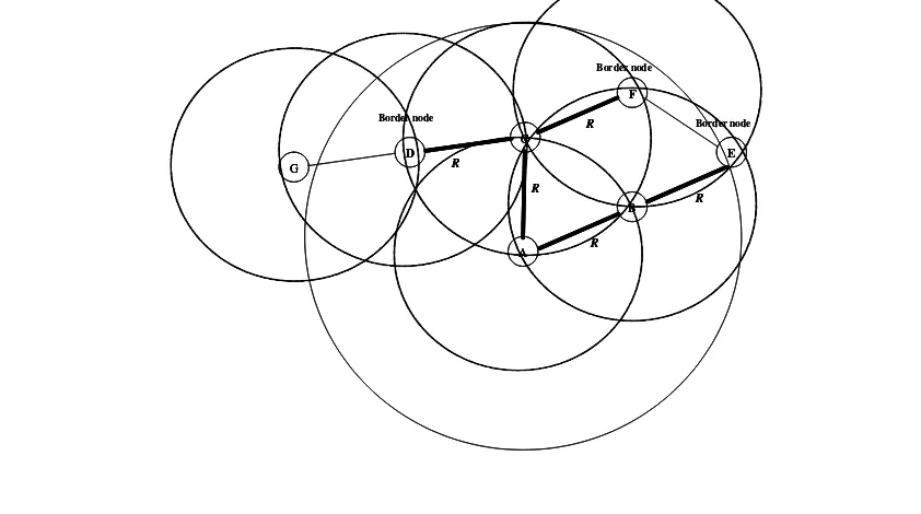
ZRP’s IARP relies on an underlying neighbor discovery protocol to detect the pres-ence and abspres-ence of neighboring nodes, and therefore, link connectivity to these nodes. Its main role is to ensure that each node within the zone has a consistent routing table that is up-to-date and reflects information on how to reach all other nodes in the zone. An example of a radius R = 2-hop routing zone (for node A) is shown in Figure 2.9; in this example nodes B through F are within the routing zone of A. Node G is outside
A’s routing zone. Also note that E can be reached by two paths from A, one with length 2-hops and one with length 3-hops. Since the minimum is less than or equal to 2, E is withinA’s routing zone. Peripheral nodes are routing zone nodes whose minimum distance to the node in question is equal exactly to the zone radius. In the above figure, nodesD,F
andE are A’s peripheral nodes. These peripheral nodes play an important role in efficient querying based on bordercasting. We note that each node maintains its own routing zone. As a result, routing zones of nearby nodes may overlap heavily.
Each node proactively tracks the topology of its routing zone through an IntrAzone Routing Protocol (IARP). IARP is derived from globally proactive link state routing pro-tocols (for example, OSPF), [28].
D
F
C
E
B
A G
R
R R
R
R
Border node
Border node
Border node
D
F
C
E
B
A G
R
R R
R
R
D D
F F
C C
E E
B B
A A G
G
R
R R
R
R
Border node
Border node
[image:32.612.88.509.147.382.2]Border node
Figure 2.9: The proactive Intrazone Routing Protocol (IARP)
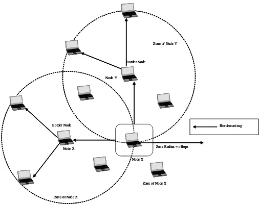
broadcast to penetrate into nodes within other zones, the border nodes in other zones that receive this messages will not propagate it further. IERP uses the bordercast resolution protocol. Bordercasting is possible as any node knows the identity and the distance to all the nodes in its routing zone by the virtue of the IARP protocol. (see Figure 2.10).
The IERP operates as follows: The source node first checks whether the destination is within its routing zone. (Again, this is possible as every node knows the content of its zone). If so, the path to the destination is known and no further route discovery processing is required. If, on the other hand, the destination is not within the source’s routing zone, the source bordercasts a route request (referred to here as a “request”) to all its peripheral nodes. Now, in turn, all the peripheral nodes execute the same algorithm: check whether the destination is within their zone. If so, a route reply (referred to here as a “reply”) is sent back to the source indicating the route to the destination. If not, the peripheral node forwards the query to its peripheral nodes, which, in turn, execute the same procedure. An example of this Route Discovery procedure is demonstrated in the figure below. As we be shown, thus, a route within a network is specified as a sequence of nodes, separated by approximately the zone radius, [29]. In Figure 2.11 the nodeA has a datagram to nodeL. Assume routing zone radius of 2-hop. Since L is not in A’s routing zone (which includes
Border Node
Border Node
Zone of Node Z
Zone of Node Y
Node Z
Node X
Zone Radius = r Hops Node Y
Zone of Node X
Bordercasting Border Node
Border Node
Zone of Node Z
Zone of Node Y
Node Z
Node X
Zone Radius = r Hops Node Y
Zone of Node X Border Node
Border Node
Zone of Node Z
Zone of Node Y
Node Z
Node X
Zone Radius = r Hops Node Y
Zone of Node X
[image:33.612.188.442.132.332.2]Bordercasting
Figure 2.10: Hybrid Approach - Zone routing protocol.
L is not found in any routing zones of these nodes, the nodes bordercast the request to their peripheral nodes. In particular, G bordercasts to K, which realizes that L is in its routing zone and returns the requested route (L−K−G−A) to the query source, namelyA.
The IERP also provides a mechanism to reactively respond to route failures. A route failure is detected by the IP when the next hop in a source route is determined to be unreachable (i.e., does not appear in the Intrazone Routing Table). Upon detection of a route failure, the IERP is alerted, and a route failure packet is generated. The route failure packet propagates back to the route’s source in the same manner as a route reply. When the route’s source receives notification of the route failure, the expired route is removed from its Interzone Routing Table. The IERP may also be configured to locally repair the damaged Interzone route by initiating a route discovery to the unreachable next hop, [27], [31].
When a route is broken due to mobility, if the source of the mobility is within the zone, it will inform all other nodes in the zone. If the source of mobility is a result of the border node or other zone nodes, then route repair in the form of a route query search is performed, or in the worst case, the source node is informed of route failure.
D E B A F C G H J C K I L Source Destination Bordercast Border node Border node Border node Bordercast Bordercast Bordercast Bordercast Bordercast Border node Border node Border node D D E E B B A A F F C C G G H H JJ C C K K I I L L Source Destination Bordercast Border node Border node Border node Bordercast Bordercast Bordercast Bordercast Bordercast Border node Border node Border node
Figure 2.11: The reactive Interzone Routing Protocol (IERP)
that the routing zone hierarchy is visible only to the ZRP entities, making bordercasting services only of use to the IERP.
Upon receipt of a (IERP) packet to be bordercasted, the BRP resolves the bordercast address into the individual IP addresses of the peripheral nodes. The received packet is then encapsulated into a BRP packet and sent to each peripheral node (via IP broadcast transmission).
The bordercasting packet delivery service is provided by the Bordercast Resolution Protocol (BRP). The BRP uses a map of an extended routing zone, provided by the lo-cal proactive Intrazone Routing Protocol (IARP), to construct bordercast (multicast) trees along which query packets are directed. (Within the context of the hybrid ZRP, the BRP is used to guide the route requests of the global reactive Interzone Routing Protocol (IERP)). The BRP employs special query control mechanisms to steer route requests away from areas of the network that have already been covered by the query. The combination of multicasting and zone based query control makes bordercasting an efficient and tunable service that is more suitable than flood searching for network probing applications like route discovery.
responsible for forwarding the packet to the next hop toward its destination, [30].
2.4
Clustering
There are several major difficulties for designing a routing protocol for MANET. Firstly, MANET has a dynamically changing topology due to the movement of mobile nodes which favors routing protocols that dynamically discover routes. Secondly, the fact that MANET lacks any structure makes IP subnetting inefficient. Thirdly, links in mobile networks could be asymmetric at times. If a routing protocol relies only on bi-directional links, the size and connectivity of the network may be severely limited; in other words, a protocol that makes use of uni-directional links can significantly reduce network partitions and improve routing performance.
Since we have mentioned until now, the networks ad hoc do not depend on some in-frastructure of preexisting communication like in the cellular systems; in this networks the mobiles nodes can be found dispersed, reason why they probably do not have direct con-nection with all other nodes. These situations determine necessary the use of intermediate nodes to reach to the destination node. A solution taken from the cellular networks is that the nodes that are in the ad hoc network self-organize themselves into clusters. Three main advantages arise here, [2]:
1. In a multihop environment, the structure of clusters facilitates reuse of resources to increase the capacity. If it does not exist overlaps of multicluster, two clusters can use the same frequency or code set if they are not neighbors.
2. The update of topology becomes hierarchical. When a mobile node changes position, this event is sufficient so that single nodes pertaining to this cluster update their topology, and not all the network.
3. The propagated and generated routing information can be reduced.
This is why many clustering algorithms have been proposed for network management.
2.4.1
Cluster Based Routing Protocol (CBRP)
is elected for each cluster to maintain cluster membership information. The protocol effi-ciently minimizes the flooding traffic during route discovery and speeds up this process as well, [7].
CBRP has the following features:
• Fully distributed operation.
• Less flooding traffic during the dynamic route discovery process.
• Explicit exploitation of uni-directional links that would otherwise be unused. • Broken routes could be repaired locally without rediscovery.
• Sub-optimal routes could be shortened as they are used.
The route shortening and local repair. Both features make use of the 2-hop-topology information maintained by each node through the broadcasting of HELLO messages. The route shortening mechanism dynamically shortens the source route of the data packet be-ing forwarded and informs the source about the better route. Local route repair patches a broken source route automatically and avoids route rediscovery by the source, [7].
However, the overhead for maintaining up-to-date information about the whole net-work’s cluster membership and inter-cluster routing information at each and every node in order to route a packet is considerable. As network topology changes from time to time due to node movement, the effort to maintain such up-to- date information is expensive and rarely justified as such global cluster membership information is obsolete long before they are used, [7]. CBRP terminology:
Node ID, is a string that uniquely identifies a particular mobile node. Node IDs must be totally ordered. In CBRP, we use a node’s IP address as its ID for purposes of routing and interoperability with fixed networks.
Cluster, a cluster consists of a group of nodes with one of them elected as a cluster head. A cluster is identified by its Cluster Head ID. Clusters are either overlapping or disjoint. Each node in the network knows its corresponding Cluster Head(s) and therefore knows which cluster(s) it belongs to.
have several host clusters.
Cluster Head, a cluster head is elected in the cluster formation process for each clus-ter. Each cluster should have one and only one cluster head. The cluster head has a bi-directional link to every node in the cluster. A cluster head will have complete knowl-edge about group membership and link state information in the cluster within a bounded time once the topology within a cluster stabilizes.
Cluster Member, all nodes within a cluster EXCEPT the cluster head are called mem-bers of this cluster.
Gateway Node, any node a cluster head may use to communicate with an adjacent cluster is called a gateway node.
HELLO message, all nodes broadcast HELLO messages periodically every HELLO INTERVAL seconds; a node’s HELLO message contains its Neighbor Table and Cluster Adjacency Table. A node may sometimes broadcast a triggered HELLO message in re-sponse to some event that needs quick action.
Conceptual Data Structures
Neighbor Table.
The neighbor table is a conceptual data structure that we employ for link status sensing and cluster formation, [7]. Each entry contains:
• The ID of the neighbor that it has connectivity with and • the role of the neighbor (a cluster head or a member). • the status of that link (bi-directional or uni-directional).
Cluster Adjacency Table.
The Cluster Adjacency Table keeps information about adjacent clusters. Each entry contains, [7], [15]:
• the ID of the neighboring cluster head
• the status of the link from the gateway to the neighboring cluster head (bi-directional or uni-directional).
Two-hop Topology Database.
In CBRP, each node broadcasts its neighbor table information periodically in HELLO packets. Therefore, by examining the neighbor table from its neighbors, a node is able to gather complete information about the network topology that is at most two-hops away from itself.
Physical and Link Layer Assumptions
Each MANET node that runs CBRP is equipped with one wireless transceiver. CBRP is capable of handling multiple transceivers per host and multiple hosts per router if the concept of a router ID is introduced.
CBRP assumes omnidirectional antennas. Each packet that a node sends is broadcast into the region of its radio coverage. CBRP is designed to operate on top of a single-channel broadcast medium.
Link/Connection Status Sensing Mechanism.
Each node knows its bi-directional links to its neighbors as well as uni-directional links from its neighbors to itself. Each node periodically broadcasts its Neighbor Table in a HELLO message.
Upon receiving a HELLO message from its neighbor B, node A modifies its own Neighbor Table as follows:
1. It checks if B is already in the Neighbor Table; if not, it adds one entry for B if it has heard from B in the previous HELLO INTERVAL before. If B’s Neighbor Table contains A, A marks the link toB as bi-directional in the relevant entry else A marks the link to B as uni-directional (uni-directional from B toA).
2. If B is already in A’s Neighbor Table.
• If the link status field of B’s entry says uni-directional but A is listed B’s hello message, then change it to bi-directional.
3. Update the role of B in the Role field of B’s entry.
Each entry in the Neighbor Table is associated with a timer. A table entry will be removed if a HELLO message from the entry’s node is not received for a period of (HELLO LOSS+1)HELLO INTERVAL.
When a node’s neighborhood topology stabilizes, the Neighbor Table of a node will have complete information of all the nodes that have a bi-directional or uni-directional link to it within a bounded time. However, a node would not know to whom it has a uni-directional link. For example in Figure 2.12, the Neighbor Table of node 7 will show that 4 has a uni-directional link to it, however node 4 would not know of the existence of such a link.
8
1
4
3 6
5
7 2
Bi-directional link
1 Cluster head
2 Cluster head Uni-directional link 8
1
4
3 6
5
7 2 8
8
1 1
4 4
3
3 66
5 5
7 7
2 2
Bi-directional link
1 Cluster head
2 Cluster head Uni-directional link
Bi-directional link Bi-directional link
1 Cluster head 1 1 Cluster head
2 Cluster head 2 2 Cluster head
Uni-directional link
Figure 2.12: Link/Connection Status Sensing Mechanism
Protocol Operation
The operations of CBRP are entirely distributed. The major components are: Cluster Formation, Adjacent Cluster Discovery and Routing.
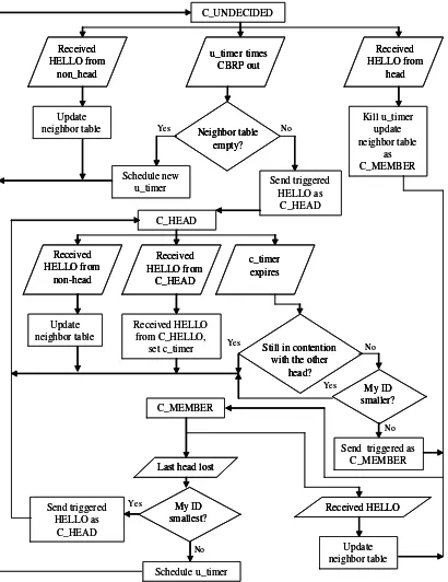
Cluster Formation
HELLO message from a Cluster Head indicating a bi-directional link in between, it aborts its u timer and sets its own status to C MEMBER, [7].
A cluster head regards all the neighbors that it has bi-directional links to as its mem-ber nodes. A node regards itself as a memmem-ber node for a particular cluster if it has a bi-directional link to the corresponding cluster head.(See Figure 2.13).
Rules for changing cluster head:
1. A non-cluster head never challenges the status of an existing cluster head, i.e. if X
is a non-cluster head node with a bi-directional link to cluster head Y, X does not become a cluster head even if it has an ID lower than Y’s.
2. When two cluster heads move next to each other (i.e. there is a bi-directional link be-tween them) over an extended period of time (for CONTENTION PERIOD seconds), then only will one of them lose its role of cluster head.
Adjacent Cluster Discovery
Cluster X and cluster Y are said to be bi-directionally linked, if any node in cluster X is bi-directionally linked to another node in cluster Y, or if there is a pair of opposite uni-directional links between any 2 nodes in clusterX and cluster Y respectively. For example in Figure 2.14, cluster 1 and cluster 2 are bi-directionally linked by the pair of links 3−>4 and 5−>6.
The goal of Adjacent Cluster Discovery is for a cluster to discover all its bi-directionally linked adjacent clusters. For this purpose, each node keeps a Cluster Adjacency Table (CAT) that records information about all its neighboring cluster heads, [7].
Routing Considerations
Routing in CBRP is based on source routing. It can be viewed as consisting of 2 phases: route discovery and the actual packets routing. Route Discovery is the mechanism whereby a node S wishing to send a packet to a destination D obtains a source route to D. the way S finds a route(or multiple routes) to D is also done by flooding.
C_UNDECIDED Update neighbor table Kill u_timer update neighbor table as C_MEMBER Neighbor table empty? Schedule new
u_timer Send triggered HELLO as
C_HEAD C_HEAD Received HELLO from non_head u_timer times CBRP out Received HELLO from head Received HELLO from non-head Received HELLO from C_HEAD c_timer expires Update neighbor table Received HELLO from C_HELLO,
set c_timer Still in contention
with the other head? C_MEMBER Send triggered HELLO as C_HEAD My ID smaller?
Send triggered as C_MEMBER Last head lost
Received HELLO Update neighbor table My ID smallest? Schedule u_timer Yes Yes Yes Yes No No No No C_UNDECIDED Update neighbor table Kill u_timer update neighbor table as C_MEMBER Neighbor table empty? Neighbor table empty? Schedule new
u_timer Send triggered HELLO as
C_HEAD C_HEAD Received HELLO from non_head Received HELLO from non_head u_timer times CBRP out u_timer times CBRP out Received HELLO from head Received HELLO from head Received HELLO from non-head Received HELLO from non-head Received HELLO from C_HEAD Received HELLO from C_HEAD c_timer expires c_timer expires Update neighbor table Received HELLO from C_HELLO,
set c_timer Still in contention
with the other head? Still in contention
with the other head? C_MEMBER Send triggered HELLO as C_HEAD My ID smaller? My ID smaller?
Send triggered as C_MEMBER Last head lost
Last head lost
[image:41.612.114.524.148.680.2]Received HELLO Received HELLO Update neighbor table My ID smallest? My ID smallest? Schedule u_timer Yes Yes Yes Yes No No No No
1
6 3
5 4
2
Bi-directional link
1 Cluster head
2 Cluster head Uni-directional link
3 4
5 6
Clusters members
7
8 11
6 6 3 3 3
5 5 4 4 4
2 2
Bi-directional link
1 Cluster head
2 Cluster head Uni-directional link
3 4
5 6
Clusters members Bi-directional link Bi-directional link
1 Cluster head
1 1 Cluster head
2 Cluster head
2 2 Cluster head
Uni-directional link
3 4
5 6
3 3 44
5 5 66
Clusters members
7 7 7
8
Figure 2.14: Adjacent Cluster Discovery
Routing
Route Shortening. Due to node movement or other reasons, a source route may become less optimal over time and should be shortened whenever possible. It works as follows: when-ever a node receives a source-routed data packet, it tries to find out the furthest node in the unvisited route that is actually its neighbor. If it succeeds, it shortens the source route accordingly and sets the S flag before forwarding the packet. When a destination node re-ceives a data packet with S flag set, it sends back a gratuitous RREP (setting the G flag in RREP) containing the shortened route to the packet source to inform it of the better route.
Route Error. When a forwarding node finds out that the next hop along the source route for an unsalvaged packet is no longer reachable, it will create a Route Error (ERR) packet and send it back to the packet source to notify it of the link failure, [7].
Local Repair. After the forwarding node detects a broken route and sends out an ERR packet, it will try to salvage the data packet the best way it can using its own local information:
1. It checks if the hop after next in the source route is reachable through an intermediate node other than the one specified as the next hop by searching through its 2-hop-topology database.
2. It checks if the unreachable next hop could be reached through an intermediate node by checking its 2-hop-topology database.
2.4.2
Access-Based Clustering Protocol (ABCP)
Nevertheless, the protocol that presents better characteristics for the process of update of the topology is the ABCP(Access-Based Clustering Protocol), since it provides generic characteristics, flexibility, rapidity in the update and a stable structure of cluster or cell. This protocol presents three main advantages that are: in which it concerns multiconnec-tions (multihop), cluster facilitates the reuse of the resources to increase the capacity of the system, this is; two to cluster can use the same frequency or code as long as these cluster, he is not neighboring; the second advantage is that when changes its position in cluster the update of all the single system is not necessary that the node updates its information, and the third advantage is that the routing information and the propagation of this can be reduced, [2], [3], with the help of the clusterhead, a hierarchical routing or network management protocol can be more easily implemented with fewer overheads.
There are two criteria for cluster initialization, and begin to partition mobile users. One is based on the node ID and the other is based on degree (the number of direct links to its neighbors). But we think that criteria based on the node ID is much more stable than the based on degree criterion; because one method for cluster maintenance is periodically running the cluster initialization algorithm regardless of the current cluster structure. The cluster updating , is realized for transmission of framework using hierarchical routing over dynamic clusters that are organized according to set of system parameters that control the size of each cluster and the number of hierarchical levels.
How we already mentioned, the clustering can facilitate the implementation such as spatial reuse, network management and routing. In a multihop environment, the resulting nonoverlapping cluster structure can be used to support the resource assignment. For in-stance, clustering provides controlled access to the channel bandwidth and scheduling of the nodes in each cluster in order to provide quality of service (QoS) support.
The objective of ABCP is build a stable cluster structure that can be deployed rapidly and do not need a mass of maintenance overhead.
Access-Based Criterion and MAC Protocol on Control Channel
want to send control messages are more than two hops away, message collision will not occur. Thus, the time slot can be spatially reused to enhance the channel efficiency.
Access-Based Clustering Criterion
Each cluster consists of one clusterhead and zero or more ordinary nodes which must be direct neighbors of the clusterhead. In the formation of the cluster structure, each node accesses the control channel to declare its intention to form a cluster. A node that success-fully sends clusrehead declaration before its one-hop neighbors do becomes clusterhead. A node that hears the clusterhead declarations from its neighbor before it has the chance to declare itself as a clusterhead becomes a member of the clusterhead node from which it receives the clusterhead declaration the first. Once a node becomes a clusterhead and has at least one cluster member, it continues to posses this role until becoming inactive.
MAC Protocol for the Control Channel: TPMA
For out-of-band signaling, one channel is dedicated to disseminate control information. The MAC protocol on single control channel has two key requirements:
1. it is distributed
2. it is to set up the channel for reliable broadcast.
The control channel is divided into fixed-size frames as shown in Figure 2.15, the format of control used in a channel within cluster in a network Ad hoc with each one of its parts that constitute it; in which two main parts can be appreciated that are; elimination slot and message slot; first it is used to synchronize the connections between nodes in a network Ad hoc which are carried out by means of Multihop or Multihop; and the second part, Message slot or groove of message that contains solely the information that is desired to send.
The defined part as elimination slot or groove of elimination this subdivided in mini-slots Ms, which are divided in three phases that are, [2].
1. RTS (Request To Send, Answer to send), in this phase each node makes their answers to indicate that it can transmit.
2. CR (Collision Report, Report of Collision), each node reports here that to happened a collision in phase RTS or no.
1 M ONE CONTROL MESSAGE
ONE CONTROL MESSAGE M
1 ONE CONTROL MESSAGE
ELIMINATION SLOT
MESSAGE SLOT
RTS CR RA
RTS: REQUEST TO SEND CR: COLLISION REPORT RA: RECEIVER AVAIBLE
1 M ONE
CONTROL MESSAGE
ONE CONTROL MESSAGE M
1 ONE CONTROL MESSAGE
1 M ONE
CONTROL MESSAGE
ONE CONTROL MESSAGE M
1
1 M ONE
CONTROL MESSAGE
ONE CONTROL MESSAGE M
1 ONE CONTROL MESSAGE
ELIMINATION SLOT
MESSAGE SLOT
RTS CR RA
RTS: REQUEST TO SEND CR: COLLISION REPORT RA: RECEIVER AVAIBLE
Figure 2.15: Format of control of channel in the Cluster of ad hoc network
Phases 1 and 3 are analogous to the RTS/CTS dialogue. However, instead of using a specific destination address (unicast), the RTS and RA indications are addressed to all one-hop neighbors (multicast). Phase 2 is used to indicate a collision occurrence if a node receives more than one RTS indications in phase 1. The following is a detailed description of the multiple access scheme.
• If a node A, wants to transmit a control message, it would wait the beginning of the next frame. In the first mini-slot of the elimination slot, node A sends an RTS in phase 1.
• If other nodes within two hops of node A also send RTS in the first mini-slot, collision will occur and be detected by one common one-hop neighbors of these transmitting nodes. The nodes that receive multiple RTSs will send a CR indication in phase 2 to indicate the collision.
• In the phase 3, the node that receives only one RTS in phase 1 will send a RA indication to acknowledge this RTS request. Phase 3 is designed to address the issue due to the restriction that a node cannot transmit and receive on the single channel simultaneously. In this phase, the node cannot transmit and receive on the single channel simultaneously.
Thus ABCP is a simple broadcast request-response with first-come-first-serve (FCFS) and it is designed from a protocol’s point of view in that it defines the message formats, describe how a node responds when a messages arrives, [2].
Protocol Description
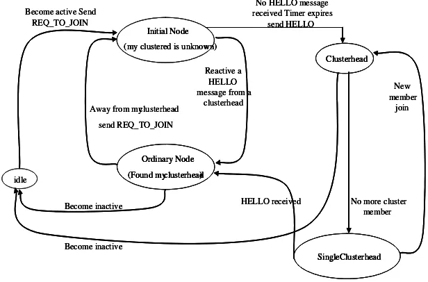
ABCP is divided into two cases for consideration. First in the ordinary node case, three situations cause an ordinary node to send a REQ TO JOIN message:
• A node initially turns on its radio units and becomes a new come to this ad hoc network;
• A node detects that a link with its clusterhead is weakening; and
• A DISCONNECT message from its clusterhead is received.
The similar form that CBRP, it wait to receive one HELLO message of some clus-terhead after that node had send a REQ TO JOIN message and set a timer. (See Figure 2.16).
idle
Initial Node
(my clustered is unknown)
Ordinary Node
(Found my clusterhead)
Clusterhead
Single Clusterhead Become active Send
REQ_TO_JOIN
Away from my clusterhead
send REQ_TO_JOIN
Reactive a HELLO message from a
clusterhead
Become inactive
Become inactive
HELLO received No more cluster member
New member
join No HELLO message
received Timer expires send HELLO
idle idle
Initial Node
(my clustered is unknown)
Ordinary Node
(Found my clusterhead)
Clusterhead
Single Clusterhead Become active Send
REQ_TO_JOIN
Away from my clusterhead
send REQ_TO_JOIN
Reactive a HELLO message from a
clusterhead
Become inactive
Become inactive
HELLO received No more cluster member
New member
join No HELLO message
received Timer expires send HELLO Initial Node
(my clustered is unknown)
Ordinary Node
(Found my clusterhead)
Clusterhead
Single Clusterhead Initial Node
(my clustered is unknown)
Ordinary Node
(Found my clusterhead) Ordinary Node
(Found my clusterhead)
Clusterhead Clusterhead
Single Clusterhead Single Clusterhead Become active Send
REQ_TO_JOIN
Away from my clusterhead
send REQ_TO_JOIN
Reactive a HELLO message from a
clusterhead
Become inactive
Become inactive
HELLO received No more cluster member
New member
join No HELLO message
[image:46.612.154.462.476.679.2]received Timer expires send HELLO
2.5
Connectivity
We have spoken about the need to have an Ad hoc wireless network. Related to this fact a link maintenance is needed to hold a wireless connection of two nodes, this point is very important to guaranty a good Quality of service (QoS) in the hole network, voiding errors and even the loose links. This is why, a concept widely used must be introduced, which defines communication between two nodes, this new concept is “connectivity”.
A pragmatic definition of Connectivity; is the unbiased transport of packets between two ending points. This definition gives a very general idea to us of which we wished to present like connectivity; but for the case of an Ad hoc wireless network where the nodes are geographically dispersed and where more likely a nodex cannot be connected with all others in a direct way or one hop; as a result we have h-hops to different intermediates nodes (IN) to reach our destination node; this is calledh-connectivity.
A formal definition of which we called h-connetivity is; two nodes i and j in an undirected graph are h-connected if there is a path connecting i and j in every subgraph by deleting (h-1) nodes other thani andj together with their adjacent arcs from the graph. This definition is illustrated in Figure 2.17 where in (a) nodes 1 and 2 are 6-connected, nodes 2 and 3 are 2-connectivity, and 1 and 3 are 1-connected. Graph (a) nodes 1 and 2 are 1-connected. Graph (b) nodes 1 and 3 are 2-connected. Another notion of interest is the arc connectivity, which is defined as a minimum number of arcs that must be deleted before the graph becomes disconnected, [18].
3
1 2
(a)
3
1 2
(a)
3
1 2
(b)
3
1 2
(b)
Model Description
In this chapter we propose a model to analyze the ad hoc network connectivity, we develop concepts to describe the connectivity that exists in this type of networks which is important to know the network organization through time and we propose a parameter called fragility with the objective of analyzing the virtual cluster robust. We also analyze statistically the total absolute connectivity
Furthermore, we explain in this chapter the Virtual Cluster-based Routing Protocol (VCRP) idea and the form to generate nodes with point processes. Finally, we present an algorithm to evaluate the ad hoc network.
3.1
Point Processes
Based on the point processes, [5], we represent stations inside a limited area; at a specific moment in time they would be considered like static or without movement. We generate nodes within the study area using a Poisson distribution in the following way, [8],
P[X =k] = γ
k
k!e
−γ, (3.1)
where γ is the average number of points per unit area, and X is the random variable for the number of nodesk=0,1,2,...
If we suppose that we have a square area with sides of length Lthen the total area is denoted asAtotal=L
2
, and the average number of points will be given by
γ =λAtotal, (3.2)