Modelling and simulation of the dynamics of near earth asteroids

Master of Science in Mechatronic Engineering

Master of Science Thesis

Modelling and Simulation of the

Dynamics of Near Earth Asteroids

Supervisors

Prof. Candido Fabrizio Pirri

Prof. Enrico Canuto

Candidate

Jorge Alfredo

Alvarez Guzman

Research Mentor

NASA Jet Propulsion Laboratory

This research was carried out at the Jet Propulsion Laboratory, California Institute of Technology, and was sponsored by the JVSRP Student Program and the National Aeronautics and Space Administration.

Foremost, a special thanks and deep regards to my mentor Dr. Marco B. Quadrelli.

I would also like to express my gratitude to Dr. Abhi Jain, Dr. Jonathan Cameron, Dr. Bob Balaram, Steven Myint, Kalvin Kuo, Hiro Ono and to my fellow interns at JPL for creating a dynamic and intellectually stimulating environment at the DARTS lab, in particular to Mayank for his helpful contributions during my research.

A sincere thanks goes to my italian supervisors, professors Fabrizio Pirri and Enrico Canuto, for giving me the opportunity to have such an edifying experience and for giving me some insight of the field of the research.

I would like to thank Magda, for her support and help during the writing process of this thesis.

This research project was aimed to study the main external perturbations that in-fluence the dynamics of Near Earth Asteroids (NEA) and implement their respective models into the DSENDSEduSims simulation platform.

Initially, the background theory of the dynamics of asteroids is presented. In-troducing the concept of the two-body problem (Sun-asteroid) and the external perturbations that affect the orbital dynamics and the attitude of the small-body. Thefirst goal of this thesis was the implementation of the Solar Radiation Pressure (SRP) model of force and torque, that can be applied to the irregular shape of an asteroid, in order to create a Python[22] function that feeds up the global simulation.

The second goal was simulating the dynamics of a specific NEA comparing two different test cases, one for the free response and the other for the forced response of the system. Consequently a study of the effects of the SRP in the behaviour of the state vector, attitude and orbital elements over time was performed. For this purpose an appropriate shape model of the asteroid, divided into finite elements of area, was adopted.

The third goal of the research was modelling the shadow effects on asteroids in order to determine individual non-illuminated areas. It may occur in two ways, the first is the self-shadowing effects that appear as a result of the irregular shape of the small-body. The second case occurs when other celestial or non celestial body enter the path of the sunlight creating shadows in the asteroid and therefore introducing small changes in the orbital dynamics.

Acknowledgements iii

Summary iv

1 Introduction 1

1.1 Near Earth Asteroids Overview . . . 1

1.2 Hypothesis . . . 4

1.3 Simulation outline . . . 4

2 Dynamics of Asteroids 7 2.1 Orbital Dynamics . . . 7

2.1.1 Reference frames . . . 7

2.1.2 Two-body problem . . . 10

2.1.3 Classical Orbital Elements . . . 13

2.1.4 Free response . . . 13

2.1.5 Converting between State Vector and COE . . . 17

2.2 Dynamic Equations . . . 19

2.3 External Perturbations on Asteroids . . . 20

3 Solar Radiation Pressure 23 3.1 Rigid Body Model . . . 24

3.2 Finite Elements of Area Model . . . 25

3.3 Solar Sail Model . . . 26

3.4 Implemented Solar Radiation Pressure Model . . . 28

4 Planetary Gravity 29 4.1 Gravitational Potential . . . 29

4.1.1 Spherical Harmonics . . . 30

4.1.2 Normalised Associated Legendre Functions . . . 31

4.2 Gravitational Acceleration Vector . . . 31

5 Shape Model of Asteroids 37

5.1 NASA Shape Models . . . 37

5.2 Gaussian Random Spheres . . . 38

6 Tests and Results 43 6.1 Asteroid Dynamics . . . 43

6.2 Thin Solar Sail . . . 55

6.3 Shadowing Effects . . . 58

6.3.1 Theoretical Method . . . 58

6.3.2 Implementation . . . 58

6.3.3 Shadowing Function . . . 59

7 Conclusions and Future Work 63 A Quaternion definitions 65 A.1 Quaternion representation . . . 65

A.2 Quaternion math . . . 66

A.2.1 Norm . . . 66

A.2.2 Normalization . . . 66

A.2.3 Conjugate . . . 66

A.2.4 Addition . . . 67

1.1 Near Earth Objects Classification. q, Q, P and a represent the per-ihelion radius, aphelion radius, orbit period, and semi-major axis

re-spectively. [22] . . . 4

1.2 ExternalForce Module Description . . . 6

2.1 Definition of the Classical Orbital Elements . . . 14

2.2 Type of conic section . . . 15

2.3 Probabilistic error modelling of environmental forces on the Galileo spacecraft [N] [12] . . . 21

2.4 Probabilistic error modelling of secular precessional torques on the Galileo spacecraft [Nm] [12] . . . 22

4.1 Variation of gravitational potential and gravitational acceleration of the Earth with the degree . . . 34

4.2 Variation of Moon’s gravitational potential and gravitational acceler-ation with the degree . . . 35

5.1 Gaussian random sphere (1620) Geographos parameters . . . 41

6.1 Initial orbital elements of asteroid (1620) Geographos . . . 43

6.2 Initial state vector of the CoM of asteroid (1620) Geographos . . . 44

6.3 Initial attitude of asteroid (1620) Geographos referred to the body frame . . . 44

1.1 Asteroid and comet locations in their heliocentric orbits [Credit: P.

Chodas, NASA/JPL-Caltech] . . . 2

1.2 Near Earth Asteroid (1620) Geographos Orbit [Courtesy NASA/JPL-Caltech] . . . 3

1.3 Asteroid Distribution in the Inner Solar System [Credit: Alan Cham-berlin, NASA/JPL-Caltech] . . . 3

2.1 Coordinate reference frames [Courtesy NASA/JPL-Caltech] . . . 8

2.2 Body-fixed reference frame [Courtesy Enrico Canuto] . . . 9

2.3 Two-body problem geometry [Courtesy Enrico Canuto] . . . 10

2.4 Classical Orbital Elements [11] . . . 13

2.5 Eccentric and Mean anomaly [1] . . . 16

2.6 "Bell Curve" Standard Normal (Gaussian) Distribution [20] . . . 22

3.1 Components of Reflection [18] . . . 23

3.2 Diagram of vectors for the non-ideal solar sail[21] . . . 26

5.1 (1620) Geographos Radar-based Polyhedron Shape Model . . . 38

5.2 Polyhedron-based model of asteroid (1620) Geographos . . . 41

6.1 Orbital trajectory of the centre-of-mass of asteroid (1620) Geographos 45 6.2 (1620) Geographos CoM Position [AU] vs Simulation Time [yr] . . . . 46

6.3 (1620) Geographos CoM Velocity hm_si vs Simulation Time [yr] . . . . 47

6.4 (1620) Geographos CoM Acceleration hm s2 i vs Simulation Time [yr] . . 48

6.5 (1620) Geographos body-frame quaternion vs Simulation Time [yr] . . 49

6.6 (1620) Geographos Orbital Elements vs Simulation Time [yr] . . . 50

6.7 (1620) Geographos Perturbation in Orbital Elements vs Simulation Time [yr] . . . 51

6.8 (1620) Geographos Gravitational Force [N] vs Simulation Time [yr] . 52 6.9 (1620) Geographos SRP Force [N] vs Simulation Time [yr] . . . 53

6.10 (1620) Geographos SRP Torque [Nm] vs Simulation Time [yr] . . . . 54

6.11 Solar sail Finite Element Model . . . 55

6.12 Force exerted on a 100 x 100 m2 _{square solar sail at 1 AU . . . 56}

6.13 Force Error [N] vs Incident Angle [deg] . . . 57

Introduction

This chapter is intended to provide the reader with both a basic overview of the subject of this dissertation and a familiarisation with the motivation of the study, simulation environment and developed routines.

1.1

Near Earth Asteroids Overview

Asteroids are small bodies in the solar system that orbit the Sun, which means that their orbits are heliocentric as is the case for all of the planets in the solar system. They are composed of rock and metals and have irregular shapes due to the fact that they are not as massive as planets, as a result of this they may rotate in peculiar ways. They are mainly located in the main belt (between the orbits of Mars and Jupiter) as can be seen in Figure 1.1. For a more specific look at their distribution in the inner solar system please see Figure 1.3, in which they are classified depending on the eccentricity and semi-major axis of their elliptical orbits. These parameters indicate how much they deviate from a circular orbit and what is the distance from the centre to the farthest point of the orbit respectively (Orbital Elements will be further explained in Chapter 2). Nevertheless, the proximity of some of these bodies with the planet Earth prompt to the definition of Near Earth Asteroids.

Near Earth Asteroids (NEA) are asteroids whose heliocentric orbits cross the Earth’s orbit and its closest approach to the Sun is below 1.3 AU1_{, as is displayed}

Figure 1.1: Asteroid and comet locations in their heliocentric orbits [Credit: P. Chodas, NASA/JPL-Caltech]

from its formation process and their composition has not changed in billions of years. They are usually classified, depending on their heliocentric orbits, as a subclass of the bigger group of Near Earth Objects (NEO) that contain also the Near Earth Comets (NEC) as reported in Table 1.1. They differ with the latter because of their formation, composition, orbit and stability of the surface.

1

1 AU = 149,597,870.700 km (mean distance between the Earth and the Sun)[28].

2

Figure 1.2: Near Earth Asteroid (1620) Geographos Orbit [Courtesy NASA/JPL-Caltech]

Group Description Definition

NEC Near Earth Comets q <1.3 [AU]

P <200 [yr2_]

NEA Near Earth Asteroids q <1.3 [AU]

Atiras NEAs whose orbits are contained en-tirely with the orbit of the Earth (named after asteroid 163693 Atira).

a <1.0 [AU] Q <0.983 [AU]

Atens Earth-crossing NEAs with semi-major axes smaller than Earth’s (named after asteroid 2062 Aten).

a >1.0 [AU] Q >0.983 [AU]

Apollos Earth-crossing NEAs with semi-major axes larger than Earth’s (named after asteroid 1862 Apollo).

a >1.0 [AU]

1.017< q <1.3 [AU]

Amors Earth-approaching NEAs with orbits exterior to Earth’s but interior to Mars’ (named after asteroid 1221 Amor).

a >1.0 [AU] q <1.017 [AU]

PHAs Potentially Hazardous Asteriods: NEAs whose Minimum Orbit Intersec-tion Distance (MOID) with the Earth is 0.05 AU or less and whose absolute magnitude (H) is 22.0 or brighter.

M OID _≤0.05 [AU] H _≤22.0

Table 1.1: Near Earth Objects Classification. q, Q, P and a represent the perihelion radius, aphelion radius, orbit period, and semi-major axis respectively. [22]

1.2

Hypothesis

The aim of this thesis is to give the reader the sufficient insight into the research de-veloped, in which the global objective was to implement a model within the simulat-ing platform for each of the considerableexternal perturbations (forces and torques) acting on an asteroid. The starting hypothesis is that the dynamics of NEA, other than the gravitational force of the Sun, are predominantly affected by the Solar Radiation Pressure (SRP) and the gravitational force exerted by the planet Earth and the Moon.

1.3

Simulation outline

developed at the Jet Propulsion Laboratory (JPL). In Figure 1.2 a description of the developed ExternalForce module is presented. It contains the principal scripts, rou-tines and functions necessary for the simulation of the theory that will be described in the following Chapters. All of the scripts were builded up using Python[26] as the programming language.

3

Folder Description

OrbitalParameters Folder containing Python functions to transform from Clas-sical Orbital Elements to state vector (COE2rv.py) or viceversa (rv2COE.py). PerturbationCOE.pyis a function to calculate the perturbation in the COE.

SolarPressure Folder containing all the scripts needed to compute the Solar Radiation Pressure. SolarPressure.py,

SolarPressureFEM.py and SolarPressureSolarSail.py

contain the models of tested versions of the SRP.

ShapeModels Folder containing the shape models of asteroids as they were adapted from the source files found at http://pds. nasa.gov/. Including the shape model of asteroid (1620) Geographos.

Shadowing Folder containing all the scripts that compute the shadow-ing effect. Examples for asteroid (1620) Geographos, an ideal Solar Sail and a primitive object (sphere) have been written. test_graphical.py displays the rendered image of the asteroid with the collisions and the shadowed areas.

test_nongraphical.pyprints the collision positions. PlanetaryGravity Folder containing scripts that calculate the gravitational

potential and acceleration of the Earth and the Moon us-ing spherical harmonics. Data input from the Earth Grav-itational Model (EGM2008) and Lunar Prospector mission (LP150) has been used. LegendreFunctions.pyis a func-tion that calculated the normalised associated Legendre polynomials needed to compute the spherical harmonics.

sphericalharmonics.py is a recursive function that cal-culates the gravitational potential and acceleration.

test Folder containing a diversity of test performed using SRP.

test_1620Geographosimplements the orbital dynamics of asteroid (1620) Geographos and measures the effect of SRP.

test_SolarSail implements a validating test case for the SRP model of a Solar Sail.

Dynamics of Asteroids

In this chapter the reader will be introduced to the framework of the dynamics of asteroids, as they constitute the base for this thesis project. Initially, an outline of the orbital dynamics of the asteroid will be provided, delineating the main reference frames needed in our particular problem, along with the parameters that characterise the gravitational motion between the celestial bodies. Afterwards, the dynamic equations that govern the system will be reported, giving significant importance to the attitude dynamics of the asteroid. Finally, there will be a description of the principal external perturbations acting on the small-body, making an assessment on the focus of our study in the following chapters.

2.1

Orbital Dynamics

The orbital dynamics of the Center of Mass (CoM) of an asteroid can be seen in two parts. First, the free response of the system is characterised by the Sun’s gravitational force. It defines the motion of the asteroid, an elliptical trajectory with the Sun in one of the focus. Second, other external forces and torques will be seen as perturbations, such as the Solar Radiation Pressure (SRP) and the Planetary Gravity. The ensemble of these perturbations define the forced response of the system.

2.1.1

Reference frames

stated next:

• The first one is the Ecliptic, a quasi-inertial plane defined by the apparent motion of the Sun during the year. Its marginal change is due to lunar and solar precession, nutation and other planetary perturbations.

• The second one is the Celestial Equator, a non-inertial plane defined by the projection of Earth’s equator. It has an obliquity (ǫ) of 23.44 degrees with respect to the former.

Figure 2.1: Coordinate reference frames [Courtesy NASA/JPL-Caltech]

A standard Ecliptic plane is often used at the J2000.0 epoch on January 1, 2000, 11:58:55.816 UTC. The reference direction is the Vernal equinox (γ),

which is the point on the Celestial Sphere at the intersection of the Celestial Equator and the Ecliptic, where the Sun crosses the Equator from south to north in its apparent annual motion along the Ecliptic[3]. This reference frame (otherwise calledInternational Celestial Reference Frame) is considered to be inertial, and it is written as:

Where the origin O is the CoM of the solar system. The plane formed by {O,ˆiJ,ˆjJ} is aligned with the Equator (Mean Equator), and ˆiJ points to the

Vernal equinox (Mean equinox). The Julian J2000 RJ reference frame is used

on the DSENDSEdu platform.

The other important reference frames to be defined are:

• The body-fixed reference frame (body-frame), is defined by an origin and two points that define the pole and the orthogonal plane. Can be formalised as follows:

Rb ={C,ˆb1,ˆb2,ˆb3}

Where, as displayed in Figure 2.2, C is the CoM of the rigid body (asteroid in our case). ˆb3 = _|CP_CP1_1| is unit vector in the direction of the pole. ˆb1 = _|CP_CP2_2| is

the unit vector defined by a point P2 that lies in the orthogonal plane (Π) to

ˆ

b3. And ˆb2 = ˆb3׈b1 is simply constructed to be orthogonal to both ˆb3 and ˆb1.

Figure 2.2: Body-fixed reference frame [Courtesy Enrico Canuto]

Rl ={C,ˆl1,ˆl2,ˆl3}

Where ˆl3 lies along the heliocentric radius vector to the asteroid, and is positive

towards the centre of the Sun. ˆl1lies in the vertical orbital plane, perpendicular

to ˆl3 and positive in the direction of the asteroid motion. ˆl2 = ˆl3׈l1 completes

the right handed orthogonal set of unit vectors, similar to the body-frame case.

• The Perifocal Reference Frame (PQW), quasi-inertial Sun-centered reference frame given by:

RP QW ={O,p,ˆ q,ˆ wˆ}

Where its origin O as previously said is the CoM of the Sun. ˆp = e_e is the unit vector in the direction of the perihelion of the elliptical orbit (given by the eccentricity vector e). wˆ = h_h is the unit vector given by the angular momentum vector (h). And ˆq= ˆw_×pˆcompletes the right handed orthogonal set of unit vectors.

2.1.2

Two-body problem

The two-body problem describes the motion of two bodies in mutual gravitational attraction. These two bodies may have an arbitrarily shape and mass, but for the scope of this thesis is restricted to study the dynamics of an asteroid m1, about a

massive and nearly spherically-symmetric body (Sun), m0.

Figure 2.3: Two-body problem geometry [Courtesy Enrico Canuto]

In Figure 2.3 the problem is illustrated. The position and velocity are defined in an inertial frame R_{O,ˆi1,ˆi2,ˆi3}, therefore the state vector of the Sun and asteroid

Newton’s law of universal gravitation states that any two bodies attract one another with a force proportional to the product of their masses and inversely pro-portional to the square of the distance between. Defining the relative position be-tween them, r =r1−r0, its magnitude,r=|r|, and the universal gravity constant,

G= 6.67259_·10−11_[ m3

kg s2][23], the mathematical equations in our case are defined as:

Fg0 =

Gm0m1

r2

r

r (2.1)

Fg1 =−

Gm0m1

r2

r

r (2.2)

Applying Newton’s second law, using the gravitational forces in Equations 2.1 and 2.2, and with the forcesF0andF1being the external perturbations, we describe

the system in a set of six equations per body. Where the state variables, _{r₀, v_0} and _{r1, v1}, are written as follows:

˙

r₀ =v₀ (2.3)

˙ v0 =

Gm0m1

m0r3

r+ F0 m0

(2.4)

˙

r1 =v1 (2.5)

˙ v1 =−

Gm0m1

m1r3

r+ F1 m1

(2.6)

With initial conditions:

r0(0) =r00, v0(0) =v00, r1(0) =r10, v1(0) =v10

Making a linear change of variables employing the relative motion between the two bodies, r = r_{1 −}r₀ and v = v₁₋v₀, we find a new set of six equations with state variables _{r, v_}, in this manner:

˙

r = ˙r₁₋r˙₀ =v₁₋v₀ =v (2.7)

˙

v = ˙v₁₋v˙₀ =₋G(m0+m1)

r3 r+

F₁ m1 −

F₀ m0

(2.8)

It is convenient to find the state vector of the CoM. Performing another linear change of variables, we define the position and velocity of the CoM in this way:

rCoM =

m0

m0+m1

r0 +

m1

m0+m1

vCoM =

m0

m0+m1

v0+

m1

m0+m1

v1 (2.10)

Using Equations 2.3, 2.4, 2.5, 2.6 and Equations 2.9, 2.10 the set of equations for the state vector of the CoM is presented, thus and thus:

˙

rCoM =

m0

m0+m1

˙ r0+

m1

m0+m1

˙

r1 =vCoM (2.11)

˙

v_CoM = m0 m0+m1

˙

v₀+ m1 m0+m1

˙

v₁ = F0+F1 m0+m1

(2.12)

From Equations 2.11 and 2.12, it is confirmed that the gravitational force is internal to the system since the set of equations of the CoM does not depend on it, but depends only on the external forces applied to the bodies.

Moreover, with the mass of the asteroid being negligible compared to the mass of the Sun (m0 >> m1) and assuming finite external forces, Equations 2.8 and 2.12

simplify, the new set of equations therefore is rewritten as follows:

˙

r=v (2.13)

˙

v _{≈ −}Gm0 r3 r+

F1

m1

=₋µ r3r+

F1

m1

(2.14)

˙

rCoM =vCoM (2.15)

˙

vCoM ≈0 (2.16)

With initial conditions:

r(0) =r0, v(0) =v0, rCoM(0) =rCoM0, vCoM(0) =vCoM0

Where µ = Gm0 = 1.32712440018·1020[m 3

s2][23] is the standard gravitational

parameter of the Sun in our specific case. Since the acceleration of the CoM ap-proximates to zero (Equation 2.16),rCoM may be selected as the centre of an inertial

2.1.3

Classical Orbital Elements

In order to describe the asteroid orbital dynamics it is necessary first to characterise the Classical Orbital Elements (COE) that are required to outline a specific orbit. These elements are considered in a two-body classical system, one of the bodies being the Sun and the other an asteroid orbiting the first one. In general it takes six parameters to uniquely define an orbit and its relative state vector. The six Keplerian classical elements used to describe the motion of a celestial body are reported in Table 2.1. In Figure 2.4 the orbit of the Celestial body is displayed with its respective orbital elements. In this case, as stated in Section 2.1.1, the plane of reference is the standard J2000 Ecliptic plane, and the reference direction is the Vernal Equinox.

Figure 2.4: Classical Orbital Elements [11]

2.1.4

Free response

In order to obtain the free response behaviour of the system, Equations 2.13 and 2.14 are simplified by setting the input from the external forces to zero. The following equations are obtained:

˙

r=v, r(0) =r₀ (2.17)

˙

v =₋µ

Parameter Description

Semimajor-axis (a) Defines the size of the orbit Eccentricity (e) Defines the shape of the orbit

Inclination (i) Defines the inclination of the orbit with respect to the reference (ecliptic) plane measured from the ascending node Argument of the perihelion (ω) Defines the orientation of the orbit in

the orbital plane, as an angle measured from the ascending node to the perihe-lion

Longitude of the Ascending Node (Ω) Defines the location of the ascending and descending orbit locations with re-spect to the reference (ecliptic) plane True Anomaly (ν) Defines where the body is within the

orbit with respect to perihelion

Table 2.1: Definition of the Classical Orbital Elements

It is convenient then to define the angular momentum vector, h, of the asteroid with respect to the Sun, and its time derivative as follow:

h=r_×v (2.19)

˙

h=r_×v˙ + ˙r_×v = 0 (2.20)

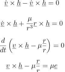
Since the time derivative of the angular momentum vector in Equation 2.20 is zero due to cross-product properties, the orbital plane can be considered as an inertial frame of reference. Now we consider the following equation:

˙

v_×h₋v˙ _×h= 0

˙

v_×h+ µ

r3r×h= 0

d dt

v_×h₋µr r

= 0

v_×h₋µr

r =µe (2.21)

is constant, lies on the orbital plane and points out to the perihelion.

Multiplying both sides of Equation 2.21 by rT _{we may find:}

rT_(v×h)− µ

rr

T_{r =µr}T_e

Applying mixed properties:

h2 ₋µr(t) =µ r(t)ecos(ν(t))

Finally finding an expression for the radius of the orbit as follows:

r(t) = p

1 +ecos(ν(t)) (2.22)

Equation 2.22 is in fact theorbit equation, otherwise named trajectory equation. Where p = h2

µ is called parameter. e = |e|, as seen in Table 2.1 is the eccentricity

of the orbit. ν(t), the angle between r and e, is the true anomaly, also reported in Table 2.1. And h = _|h_| is the magnitude of the angular momentum vector. Furthermore this equation describes the shape and size of the orbit, indicating that all asteroid orbits are conic sections: ellipses, circles, parabolas and hyperbolas.

Conic Section Eccentricity

Circle e= 0

Ellipse 0< e < 1

Parabola e= 1

Hyperbola e >1

Table 2.2: Type of conic section

Table 2.2 shows the different type of conic sections, and therefore all of the possible orbits that the asteroid may describe depending on the eccentricity.

Normally the motion of the asteroid within the orbit is described by the true anomaly (ν), but it can be replaced by the eccentric anomaly (E), which is the angular distance between the perihelion and the projection of the position of the elliptical orbit into its auxiliary circle of radius a, measured from the centre of the orbit (as seen in Figure 2.5). Now we present the differential equation that defines this motion, a modified version of Kepler’s equation, like this:

˙

E(t)(1₋e cos(E(t))) =ω0, E(0) = 0 (2.23)

Figure 2.5: Eccentric and Mean anomaly [1]

ω0 =

r_µ

a3 [rad/s]

p0 =

2π ω0

[s]

The mean angular rate is the constant angular rate that the asteroid would have in a circular orbit (e= 0), and the mean angular period would be its period in such case. Solving Equation 2.23 we find the Free Response equation:

E(t) =e sin(E(t)) +ω0(t−t0), t ≥t0 (2.24)

r(t) =a(1₋e cos(E(t))) (2.25)

The linear part of Equation 2.24 is called mean anomaly, M(t) = ω0(t−t0).

In the particular case of a circular orbit, since we have zero eccentricity (e = 0), Equation 2.24 and Equation 2.25 simplify, and therefore we obtain:

E(t) = ω0(t−t0), t≥t0 (2.26)

As expected the radius of the orbit is equivalent toa, and in this case the eccentric anomaly and the mean anomaly are identical.

2.1.5

Converting between State Vector and COE

From the COE it is possible to calculate the orbital state vector. The state vector of position (r) and velocity (v), previously employed in Equations 2.13 and 2.14, uniquely determine the trajectory of the orbit of an asteroid. They may be ex-pressed in cartesian coordinates with respect to the inertial frame, as follows:

r=x1ˆi+x2ˆj+x3ˆk

v =v1ˆi+v2ˆj +v3ˆk

A couple of algorithms to transform from COE to state vector and vice versa were implemented as Python functions. Both of them are of vital importance during our simulations. The state vector is needed to compute the orbital dynamics, and the COE allow us to study the orbital dynamics and its variation over time.

• State Vector to COE Algorithm

The algorithm to transform from the State Vector to COE found in [25] is presented:

(a, e, i,Ω, ω, ν) = rv2COE(r, v)

h=r_×v

n = ˆk_×h

e=

v2₋ µ r

r₋(r_·v)v µ

ξ = v

2

2 − µ r

If e /= 1.0 then:

p= (1₋e2)

else:

p= h

2

µ and a=∞

cos(i) = hk |h_|

cos(Ω) = ni

|n_| if(nj <0)thenΩ = 360

◦

−Ω

cos(ω) = n·e

|n_||e_| if(ek <0)then ω = 360

◦

−ω

cos(ν) = e·r

|e_||r_| if(r·v <0)then ν = 360

◦

−ν

• COE to State Vector Algorithm

The algorithm to transform from COE to the State Vector found in [25] is presented:

(r, v) = COE2rv(a, e, i,Ω, ω, ν)

rP QW =

"

pcos(ν) 1 +ecos(ν),

psin(ν) 1 +ecos(ν),0

#

vP QW =

" − s µ psin(ν), µ

p(e+ cos(ν)),0

#

r= [P QW2IJK]rP QW

[P QW2IJK] =

   

cΩcΩ−sΩsΩci −cΩsΩ−sΩcΩci sΩsi

sΩcΩ+cΩsΩci −sΩsΩ+cΩcΩci −cΩsi

sΩsi cΩsi ci

   

Where cΩ =cos(Ω), sΩ =sin(Ω), ci =cos(i) and si =sin(i).

2.2

Dynamic Equations

In order to study the motion of an asteroid or any other celestial body it is important to accurately define the dynamic equations that fully represent our system. In our case a Newtonian-Keplerian approach has been used to formulate the differential equations that fully describe the six degrees of freedom (DOF) in the two-body system, allowing us to calculate the state vector and the attitude of the asteroid, in the following way:

˙

r=v (2.28)

¨

r =₋µ

r3r+ap (2.29)

ap =

P

fp

m (2.30)

˙

q =H(q)ω (2.31)

I_·ω˙ +ω_×(I_·ω) = τ (2.32)

τ =X

τp =

X

cp×fp

(2.33)

Wherer andv form the state vector, they are the position and velocity of respec-tively. q and ω are the attitude quaternion and angular velocity correspondingly. I

is the moment of inertia tensor. τ is the total torque. fp and τp are the external

perturbations, in the fashion of forces and torques respectively. apis the acceleration

vector due to the combined effect of all the external forces. AndH(q) is defined by:

H(q) = 1 2

 

q×

v +q3I3×3

−qT v

 

WhereI3×3 is the 3 x 3 identity matrix andq×_v is the cross-product matrix given

q×_v =

   

0 ₋q2 q1

q2 0 −q0

−q1 q0 0

   

The DSENDSEdu platform simplifies our problem, due to the fact that it has been intrinsically designed to solve these differential equations and obtain at any point the state vector and the attitude of the body. Our scope will be that of correctly defining the initial settings and external inputs of our system.

2.3

External Perturbations on Asteroids

The motion of the asteroid is subject to external forces and torques that determine the forced response of the system. They are classified into gravitational and non-gravitational perturbations, depending on its nature. The main forces and torques considered as perturbations are:

• Solar Radiation Pressure: non gravitational perturbation caused by the elec-tromagnetic radiation of the Sun. The photon flux originating from the Sun produces an effective pressure[2] on the celestial bodies that intercept it. This pressure is further traduced into a force and torque perturbation. Its concept will be deepen in Chapter 3.

• Planetary Gravity: gravitational perturbation caused by a third-body gravita-tional potential. It has particular importance during closeflybysof Planets or their natural satellites. Its theory will be expanded in Chapter 4.

• Solar Wind: the Sun is losing mass in form of the solar wind, which has affected its evolution from its birth and will continue to do so until its death. The surface of the Sun is called the photosphere, above which lies the Sun’s atmosphere, known as the corona. The solar wind forms in the corona and is caused by high pressure in the corona relative to the low pressure far from the Sun in the interstellar medium. Solar wind is an ionized gas made up primarily of protons and electrons with minor ions in amounts similar to those in the corona. The rotation of the sun results in the lines of magnetic flux in the solar wind being drawn into Archimedian spirals1_{. This is because the}

Sun revolves once every _∼25.5 days while it takes solar wind several days to reach 1 AU[24]. Therefore the Sun rotates through a significant angle during the time it takes the solar wind to reach an asteroid.

In Tables 2.3 and 2.4 an overview of the probabilistic error of all the important perturbations for a Near Earth environment is presented[12]. The survey is applied to the Galileo spacecraft, but for our analysis it provides trustworthy information of the contribution of the different perturbations in the specific environment of a NEA.

It is assumed that all of the error sources or the combined effect of the error sources have a normal (Gaussian) distribution[12]. The mean and three standard deviations (3σ) values are displayed. As can be seen in Figure 2.6, 99.73% of val-ues are within three standard deviations of the mean, therefore we have a good approximation of the actual value of the external perturbations.

Near Earth (10RE)

Source Mean 3σ

Solar Radiation Pressure 9.0_×10−5 _2.6×10−5

Planet Thermal Radiation 7.8_×10−8 _5.2×10−8

Solar Wind 3.1_×10−8 _1.6×10−8

Newtonian Drag 7.9_×10−11 _2.4×10−10

Table 2.3: Probabilistic error modelling of environmental forces on the Galileo spacecraft [N] [12]

Our attention will now be focused on the effects of SRP and Planetary Gravity (Gravity Gradient), as they are the main sources of external perturbation to the

1

Figure 2.6: "Bell Curve" Standard Normal (Gaussian) Distribution [20]

Near Earth (10RE)

Source Mean 3σ

Solar Radiation Pressure 0 3.2_×10−7

Planet Thermal Radiation 3.5_×10−8 _2.5×10−8

Solar Wind 0 2.8_×10−10

Newtonian Drag 3.4_×10−11 _1.1×10−10

Gravity Gradient Torque 3.2_×10−7 _3.9×10−8

Table 2.4: Probabilistic error modelling of secular precessional torques on the Galileo spacecraft [Nm] [12]

Solar Radiation Pressure

In this chapter the reader will be introduced to some models of Solar Radiation Pressure (SRP). These models represent a physical approach for calculating the SRP force and torque acting on an asteroid. The complexity of such models greatly depend on the magnitude of the uncertainty and therefore how similar to the real-ity is the model meant to be. The models here presented were implemented into appropriate Python functions that feed up the overall simulation of the asteroid’s dynamics.

Figure 3.1: Components of Reflection [18]

cumulative effect over sufficiently long periods of time that make it significant[10], in particular for NEA that do not experience strong gravitational dynamics or other significant environmental forces. Sunlight has both energy and momentum, conse-quently when a photon is absorbed or reflected, momentum is exchanged[2]. Re-sultant force is a function of the exposed area and surface characteristics, which determine how the incoming photons are specularly reflected, diffusely reflected or absorbed.

3.1

Rigid Body Model

As a start the model of D.A. Vallado[25] of SRP for a rigid body is presented. This basic model, as will be seen additionally in the rest of the models, strongly depends on the area-to-mass ratio of the body. This give us a hint on what should be our scope when determining the relevance of the SRP effect on the orbital dynamics of a natural satellite. The structure of the equation is given as:

a_SR =₋pSRCRA⊙ m

rast⊙

|rast⊙|

(3.1)

Where CR is the single reflectivity coefficient, pSR is the SRP coefficient, and

A⊙ is the exposed area to the sun. And the position vector defined in an inertial

reference frame is written as:

rast⊙: position vector between asteroid and sun

|rast⊙|: magnitude of the position vector

ˆ rast⊙ =

rast⊙

|r_ast⊙|: unit vector pointing to the Sun (incident vector line)

Now, as showed in Figure 3.1, we consider the case for different components of reflection and absorption. From this analysis we obtain the following equations:

f_a =₋pSRCRaA⊙cos(φinc)ˆs (3.2)

f_rs =₋2pSRCRsA⊙cos2(φinc)ˆn (3.3)

f_rd=₋pSRCRdA⊙cos(φinc)

2

3nˆ+ ˆs

(3.4)

Where φinc is the solar-incidence angle, ˆs is the unit vector pointing in the

and diffuse reflectivities respectively. The summation of these coefficients must be equal to one (CRa+CRs+CRd = 1).

Adding the previous terms of force in Equations 3.2, 3.3 and 3.4, and assuming a Lambertian diffusion (ideal diffusely reflecting surface) we find compact equations for the SRP Force and Torque, defined by:

f_SRP =₋pSRA⊙cos(φinc)

2

C

Rd

3 +CRscos(φinc)

ˆ

n+ (1₋CRs)ˆs

(3.5)

τSRP = (rCoP −rast⊙)×f_SRP (3.6)

Where rCoP is the position of Center of Pressure (CoP) of the body, and rast⊙

corresponds to the position of the CoM of the asteroid.

3.2

Finite Elements of Area Model

In this section the SRP is modelled in a more in depth way, instead of having an estimated cross-sectional area illuminated by the Sun rays, the total area exposed to the Sun is defined as the addition of a number of finite areas. Following up the P.C. Hughes[10] model for SRP Force and Torque are presented:

f =p[(σa+σrd)Apsˆ+

2

3σrdAp+ 2σrsApp] (3.7)

g =p[(σa+σrd)cpxsˆ+

2

3σrdGp+ 2σrsGpp] (3.8)

Where Ap,cp, Ap, App,Gp and Gpp are given as:

Ap =

"

H(cos(θ))cos(θ)dA (3.9)

AprCoP =

"

H(cos(θ))cos(θ)rdA (3.10)

Ap =

"

H(cos(θ))cos(θ)dA (3.11)

App =

"

H(cos(θ))cos2(θ)dA (3.12)

Gp =

"

Gpp =

"

H(cos(θ))cos2(θ)rxdA (3.14)

Where θ is the incident angle. H(cos(θ)) is the Heaviside function (H(cos(θ)) = 1 when cos(θ)>0), it limits the calculation of the SRP to the areas that are exposed to the sun, specifically when the incident angle is ₋π

2 ≤θ ≤

π

2.

And the relative position r =rCoP −rCoM, where rCoP is the location of the CoP,

rCoM is the location of the CoM of the asteroid.

The difference between the total CoP and the CoM is what creates the applied torque to the body. If both of them would be located in the same position with respect to the body the applied torque would be zero.

The differential element of area dA = ˆndA can be decomposed in magnitude and direction.

The parametersσa,σrdandσrsare respectively the coefficients for absorption, diffuse

reflection and specular reflection.

3.3

Solar Sail Model

Figure 3.2: Diagram of vectors for the non-ideal solar sail[21]

the SRP), both of them possess high area-to-mass ratio and furthermore they must be almost perfect reflectors for the SRP to be appreciable.

Unfortunately, as considered in the previous model, the SRP force is not gener-ated by a surface with a perfect reflectivity. Therefore as can be seen in Figure 3.2 the force exerted by a non-ideal solar sail is obtained by considering reflection, ab-sorption and re-radiation by the sail.

The equations of the SRP exerted by the sail are determined by:

fn=pA((1 + ˜rs)cos2θ+Bf(1−s)˜rcosθ+ (1−˜r)

εfBf −εbBb

εf +εb

cosθ)ˆn (3.15)

ft =pA(1−˜rs)cosθsinθˆt (3.16)

For this model ˜ris the reflection coefficient,sis the fraction of specularly reflected force, ˆn is the unit vector normal to the sail surface, ˆt is the transverse unit vector to that surface, Bf and Bb are the coefficient that account for a non-Lambertian

surface in the front and back of the sail. εf andεbare the front and back emissivities.

Limiting our model to only front sail surfaces, the equation in the normal direc-tion changes as follow:

fn =pA((1 + ˜rs)cos2θ+Bf(1−s)˜rcosθ+ (1−r)B˜ fcosθ)ˆn (3.17)

Which for a coefficient Bf = 2₃ (Lambertian diffusion) turns out to be a similar

equation as the previous models.

The only notable difference between models is the notation used to describe the coefficients. For this reason and for a future test validation a coefficient relation between models is presented:

˜

r =σrd+σrs = 1−σa (3.18)

s= 1₋σ (3.19)

σrd =σ(1−σa) (3.20)

σrs= (1−σ)(1−σa) (3.21)

Whereσais the fraction absorbed andσ is the fraction that is diffusely reflected,

3.4

Implemented Solar Radiation Pressure Model

In this section simplified equations to calculate the total SRP force and torque are derived from the P.C. Hughes[10].

Replacing 3.9, 3.10, 3.11, 3.12, 3.13 and 3.14 in 3.7 we obtain:

f =p[(σa+σrd)

"

H(cosθ)cosθdAˆs+2 3σrd

"

H(cosθ)cosθdA+2σrs

"

H(cosθ)cos2θdA]

f =

"

p[(σa+σrd)H(cosθ)cosθˆs+

2

3σrdH(cosθ)cosθnˆ+ 2σrsH(cosθ)cos

2_θn]dAˆ

f =

"

pH(cosθ)cosθ[(σa+σrd)ˆs+ (

2

3σrd+ 2σrscosθ)ˆn]dA (3.22) Equation 3.22 is in fact the total SRP Force. Using this equation and the relative distance between the CoP and the CoM, we derive an expression for the the total SRP Torque perturbing the asteroid, as follows:

f_SRP =

"

pH(cos(θ)) cos(θ)[(σa+σrd)ˆs+ (

2

3σrd+ 2σrscos(θ))ˆn]dA (3.23)

τSRP =r×f_SRP (3.24)

Planetary Gravity

In the unperturbed Keplerian motion of an asteroid about the Sun, it is assumed that the dynamics of the small-body are only defined by the acceleration due to the gravity of the Sun (this concept was established in Section 2.1 as the free response of the system). In reality other planets also introduce a perturbing acceleration on the body, defined as third-body gravitational perturbations. They are usually small comparing to that of the Sun and therefore its effect is neglected. However such is not the case of our problem.

In this chapter the reader will be introduced to the gravitational acceleration exerted by other Planets or their natural satellites on asteroids. Particularly, since the subject of our study are NEA, its close flyby to the Earth and Moon makes their effect considerable compared to that of the rest of the Planets. Therefore the importance of describing the aforementioned effects in a more accurate way.

4.1

Gravitational Potential

When calculating the gravitational potential of a planet it is often assumed that the total mass of the planet (i.e. Earth), is concentrated in the center of the coordinate system, and the gravitational law [16] is written by:

¨

r=₋GM

r3 r (4.1)

this purpose a more realistic model is presented. This model involves the gradient of the gravitational potential (V) of the body[16] in the following way:

¨

r =_∇V (4.2)

with

V =G

ˆ

dm

|r₋s_| (4.3)

Equation 4.3 applies for an arbitrary mass distribution anddm =ρ(s)d3_{s is the}

mass element. Where s is the position of the individual mass element with respect to the CoM, and ρ(s) is the density of the body.

4.1.1

Spherical Harmonics

The fraction within the integral in Equation 4.3 is expanded in a series of Legendre Polynomials[16], as follows:

1 |r₋s_| =

1 r ∞ X n=0 s r n

Pn(cos(γ))

Where γ = r_rs·s is the angle between r and s, and the Legendre polynomial of degreen (Pn) is written as:

Pn(θ) =

1 2n_n!

dn

dθn(θ

2

−1)n

And the associated Legendre polynomials of degree n and order m are defined as:

Pnm(θ) = (1−θ2)m/2

dm

dθmPn(θ)

Introducing the spherical coordinates (r, θ, λ), with radius r, longitude λ, and latitudeθ, it is possible to write the planetary gravitational potential in the following form[9]:

V(r, θ, λ) = GM

r + GM r nmax X n=2 a r n n X m=0 ¯

Cnmcos(mλ) + ¯Snmsin(mλ)

¯

Pnm(θ) (4.4)

Where ¯Cnm and ¯Snm are the fully-normalised, unit-less, spherical harmonic

co-efficients of the Planet’s gravitational potential, and ¯Pnm(θ) are the normalised

4.1.2

Normalised Associated Legendre Functions

In this section a method[9] of forward recursions for the calculation of the nor-malised associated Legendre functions (polynomials) ¯Pnm(θ) is presented. The full

normalisation is given by:

¯

Pnm(θ) =

v u u

tk(2n+ 1)(n−m)!

(n+m)! Pnm(θ) (4.5)

wherek = 1 for m = 0 andk = 2 for m >0.

The full normalisation requires a recursion that computes non-sectoral (n > m) from previously computed functions. The non-sectoral terms of ¯Pnm(θ) are given as:

¯

Pnm(θ) =anmtP¯n−1,m(θ)−bnmP¯n−2,m(θ), ∀n > m (4.6)

where t=cos(θ)

anm =

v u u t

(2n+ 1)(2n+ 1) (n₋m)(n+m)

and

bnm =

v u u

t(2n+ 1)(n+m−1)(n−m−1)

(n₋m)(n+m)(2n₋3)

The sectoral (n =m) terms ¯P0,0(θ) = 1 and ¯P1,1(θ) =

√

3u serve as seed values for the recursion, where u=sin(θ).

The higher degree and order terms of ¯Pmm(θ) are computed as follow:

¯

Pmm(θ) =u

s

2m+ 1

2m P¯m−1,m−1(θ), ∀m >1 (4.7)

4.2

Gravitational Acceleration Vector

The gravitational acceleration vector, g, is calculated as the first partial derivative of the Gravitational Potential, V, with respect to the planet-fixed position vector, r. A method found in [7] for calculatingg is presented:

g _≡ ∂V

∂r (4.8)

r =     x1 x2 x3     ˆ r= r

r

Λ_≡Γ + x3H r J _≡ nmax X n=2 a r n Jn K _≡ nmax X n=2 a r n Kn H _≡ nmax X n=2 a r n Hn

Γ_≡1 +

nmax X n=2 a r n Γn

Defining the n variables as:

Jn≡ n

X

m=1

mP¯n,m

rm−1( ¯Cn,mCm−1+ ¯Sn,mSm−1)

Kn≡ − n

X

m=1

mP¯n,m

rm−1( ¯Cn,mSm−1−S¯n,mCm−1)

Hn ≡C¯n,0P¯n,1+

n

X

m=1

¯ Pn,m+1

rm ( ¯Cn,mCm+ ¯Sn,mSm)

Γn≡C¯n,0(n+ 1) ¯Pn,0+

n

X

m=1

(1 +n+m)P¯n,m

rm ( ¯Cn,mCm+ ¯Sn,mSm)

and

Cm ≡ρmcos(mλ)

Sm ≡ρmsin(mλ)

We can write a simple and compact vector equation for the gravitational accel-eration:

g =₋µ r2

   Λˆr−

    J K H         (4.9)

4.3

Earth Gravitational Model

As previously discussed in the case of the study of the orbital dynamics of NEA, it is fundamental to measure the perturbing effect caused by the gravitational potential of Earth. For this reason the Earth Gravitational Model EGM2008[19] is adopted. The EGM2008[19] model is complete to degree and order 2159. This model represents the most complete description of the Earth’s gravitational model in spherical harmonics. The ASCII file contains 2401333 formatted records with the following coefficients:

{n, m,C¯nm,S¯nm, sigmaC¯nm, sigmaS¯nm}

Wheren, is the degree, m, the order, ¯Cnm and ¯Snm are the normalised spherical

harmonic coefficients of the gravitational potential, and sigmaC¯nm and sigmaS¯nm,

their associated error standard deviations.

The scaling parameters (standard gravitational parameter, GM, and the equato-rial radius, a) associated with this model have numerical values:

GM = 3986004.415_×108hm3

s2

i

a = 6378136.3 [m]

n V[Nm

kg ] g[

m s2]

3 62459416.154 (2.245017e-18, -0.0, 9.755439150056413) 4 62459416.154 (2.245015e-18, 1.073547e-23, 9.755439171420868) 5 62459416.154 (2.234156e-18, 1.073547e-23, 9.755579372118891) 6 62459416.154 (2.245231e-18, 2.172461e-20, 9.755439283003227) 7 62459416.154 (2.225674e-18, 2.569082e-20, 9.755683211368497) 8 62459416.154 (2.214619e-18, 2.043162e-20, 9.755819689420921) 9 62459416.154 (2.212929e-18, 2.016738e-20, 9.755840385846357) 10 62459416.154 (2.221663e-18, 1.259672e-20, 9.75573408029359) 11 62459416.154 (2.222447e-18, 1.607862e-20, 9.75572457575225) 12 62459416.154 (2.214993e-18, 1.263204e-20, 9.75581447903136) 13 62459416.154 (2.215362e-18, 2.073509e-20, 9.755810051547115) 14 62459416.154 (2.213559e-18, 1.195743e-20, 9.75583166226041) 15 62459416.154 (2.210959e-18, 1.031292e-20, 9.755862738632983) 16 62459416.154 (2.209396e-18, 1.739376e-20, 9.755881374822108) 17 62459416.154 (2.206491e-18, 1.582666e-20, 9.755915959760905) 18 62459416.154 (2.211131e-18, 1.736107e-20, 9.755860821214721) 19 62459416.154 (2.214331e-18, 1.937496e-20, 9.755822848474203) 20 62459416.154 (2.214976e-18, 1.989379e-20, 9.755815219534897)

Table 4.1: Variation of gravitational potential and gravitational acceleration of the Earth with the degree

4.4

Moon Gravitational Model

The other considerable external gravitational perturbation for NEA is the gravita-tional acceleration generated by the Moon. In a similar way to the previous section, we use the Lunar Prospector mission data LP150[13]. The LP150[13] model is com-plete to the 150th degree and order. The ASCII file contains 11473 formatted records with the following coefficients:

{n, m,C¯nm,S¯nm, sigmaC¯nm, sigmaS¯nm}

Where n, is the degree, m, the order, ¯Cnm and ¯Snm are the normalised spherical

harmonic coefficients of the gravitational potential, and sigmaC¯nm and sigmaS¯nm,

The scaling parameters (standard gravitational parameter, GM, and the equato-rial radius, a) associated with this model have numerical values:

GM = 0.49028002380000_×1013hm3

s2

i

a = 1738000.0 [m]

The results of a test of the model up to the 20th degree and order, with position vector r= [0,0,1738000.0], are presented:

n V[Nm

kg ] g[

m s2]

3 2820943.75029 (-0.0, -0.0, -1.6221080516181843) 4 2820943.75029 (-0.0, -0.0, -1.6221075428218674) 5 2820943.75029 (-0.0, -0.0, -1.6220285395287453) 6 2820943.75029 (-0.0, -0.0, -1.6224252246161879) 7 2820943.75029 (-0.0, -0.0, -1.6223695327499759) 8 2820943.75029 (-0.0, -0.0, -1.6223970597650141) 9 2820943.75029 (-0.0, -0.0, -1.6221939155996075) 10 2820943.75029 (-0.0, -0.0, -1.6222233553284742) 11 2820943.75029 (-0.0, -0.0, -1.6220696886369494) 12 2820943.75029 (-0.0, -0.0, -1.6218769635476218) 13 2820943.75029 (-0.0, -0.0, -1.621945771201444) 14 2820943.75029 (-0.0, -0.0, -1.622025384358224) 15 2820943.75029 (-0.0, -0.0, -1.622145487058275) 16 2820943.75029 (-0.0, -0.0, -1.6221011972293156) 17 2820943.75029 (-0.0, -0.0, -1.6221490768703688) 18 2820943.75029 (-0.0, -0.0, -1.621871011647331) 19 2820943.75029 (-0.0, -0.0, -1.621811282914) 20 2820943.75029 (-0.0, -0.0, -1.6217564652529954)

Shape Model of Asteroids

In this chapter the reader will be introduced to the shape model of asteroids and its structure. The mentioned shape must be adequate with the models of the main external perturbations previously discussed, and will be subsequently used with major importance in the simulation of the dynamics of asteroids. For this purpose the entire surface of the small-body is divided into finite elements of area, fitting the model of SRP presented in Section 3.2. In order to accomplish this, the asteroid is modelled as a polyhedron-shaped body, a mesh containing flat facets and straight vertices. Each facet represents a finite area within the polyhedron and the vertices define the total area within each facet.

5.1

NASA Shape Models

In Figure 5.1 a model of asteroid (1620) Geographos is presented. This and sev-eral other shape models can be found in NASA’s Planetary Data System (http: //sbn.psi.edu/pds/archive/shape.html). These shape models were derived us-ing experimental data from radar or optical observations. Shape models typically have several thousands of surface triangular facets[5], increasing the number of facets increases the precision of the model but also increases the computational effort. For each asteroid there is a .obj (.tab) file with the following format:

v x1 y1 z1 v x2 y2 z2 v x3 y3 z3 ...

Figure 5.1: (1620) Geographos Radar-based Polyhedron Shape Model

Rows starting with lettervrepresent thex, y, andz-axis coordinates of each vertex, whereas rows starting with letterf represent each triangular facet and i,j, andkare the number of vertices that form the facet. The number of facetsnf and the number

of vertices nv are related by nf = 2nv −4. The radar shape model of the asteroid

(1620) Geographos shown in Figure 5.1 contains 8192 Vertices and 16380 Facets, which imply a great computational constraint. In fact when this model is used to measure the effects of SRP in the orbital and attitude dynamics of the small-body, the simulation runs slow. For this reason another approach has been used to model the asteroid’s shape.

5.2

Gaussian Random Spheres

statistical-stochastic GRS model found in [17] is presented. The three-dimensional GRS is described by:

r(ϑ, φ) =a exp

s(ϑ, φ)₋1 2β

2 _(5.1)

s(ϑ, φ) =

∞

X

l=0

l

X

m=−l

slmYlm(ϑ, φ) (5.2)

Wherea andβ are the mean radius and the standard deviation of the logradius, and Ylm’s are the orthonormal spherical harmonics. The relative standard deviation

of radius is σ=qexp(β)2 _−1.

The real and imaginary parts of the spherical harmonics coefficientsslm,m ≥0, are

independent Gaussian random variables with zero means and variances

V ar(Re(slm)) = (1 +δm0)

2π 2l+ 1Cl

V ar(Im(slm)) = (1−δm0)

2π 2l+ 1Cl

The coefficientsCl≥0 are the Legendre coefficients of the log radius covariance

function Σs, and we may write the following equation:

Σs(γ) =β2Cs(γ) =

∞

X

l=0

ClPl(cosγ)

∞

X

l=0

Cl=β2

In which Cs is the logradius correlation function, represented as:

Cs(γ) =

∞

X

l=0

clPl(cosγ),

∞

X

l=0

cl= 1

In order to implement the model, the series need to be truncated at a certain degree L high enough to maintain good precision. The two perpendicular slopes, s(ϑ) = rϑ

r and s(φ) = rφ

r , are independent Gaussian random variables with zero

mean, and standard deviation given by:

ρ=

q

Where Σ(2)

s (0) is the second derivative of the covariance function with respect to

γ. The correlation length ℓ and correlation angle Γ are defined by:

ℓ = q 1

−Cs(2)(0)

Γ = 2arcsin(1 2ℓ)

Since the focus of the algorithm will be that of creating individual shapes, it is needed to define some intrinsic parameters of the relative shape. Defining the intrinsic expectation of a function f =f(ϑ, φ) as:

E(f) = 1 4π

ˆ π

0 ˆ 2π

0

dϑdφsin(ϑ)f(ϑ, φ) (5.3)

Using Equation 5.3 it is possible to write an expression for the mean radius ˜a, standard deviation of the radius ˜σ, standard deviation of the logarithmic radius ˜β, standard deviation of slopes ˜ρ and correlation angle ˜Γ as follows:

˜

a=E(r) (5.4)

˜ ρ2 = 1

˜ a2[E(r

2₎

−E(r)2] (5.5)

˜

β2 =E[(loger)2]−[E(logee)]2 (5.6)

˜ Γ = 1

2E r2

ϑ

r2 +

r2

φ

r2_sin2_ϑ

!

(5.7)

A Python routine has been implemented in order to generate GRS that recreate the individual shape of specific asteroids using the previous equations. The shape is stored into a .obj (.tab) file with the same format (facets-vertices) as the one defined in Section 5.1. Next it will be loaded into the main routine that computes the dynamics of the asteroid, and calculates the external forces and torques. At this point it will be particularly important to measure the total SRP acting on the body, since each facet provides a unique contribute to the total perturbation.

Parameter Value

Mean radius ˜a= 1.08[km] Standard deviation of the radius σ˜ = 0.319

Standard deviation of slopes ρ˜= 0.546 Correlation angle Γ = 33.1[˜ ◦_]

Mean density ρ˜= 2.5[_cmg3]

Table 5.1: Gaussian random sphere (1620) Geographos parameters

Tests and Results

In this chapter validating tests of the implemented Python[26] functions and their respective results will be reported. This chapter includes three main sections. The first one is dedicated to the test of the asteroid’s dynamics and its behaviour over time, performing an assessment of the importance of the main external perturba-tions. The second one aims to validates the SRP model for a solar sail, contrasting the results with trusted bibliography. And the third one explores the concept of shadowing effects, and its relative importance when calculating the total SRP act-ing on an asteroid.

6.1

Asteroid Dynamics

In this section the results from the simulation of the orbital dynamics of asteroid (1620) Geographos will be presented. The following initial orbital parameters found in [5] are assumed:

Parameter Value

Semi-major axis a = 1.24547AU

Eccentricity e= 0.3354

Inclination i= 13.34◦

Argument of the perihelion ω = 277.8◦

Longitude of ascending node Ω = 337.3◦

True anomaly ν = 10◦

Table 6.1: Initial orbital elements of asteroid (1620) Geographos

frame is found:

State vector Value

Position r0 = [−9385183996.563,−120902054235.237,−27307229916.384]m

Velocity v0 = [37304.738,−5110.708,2295.700]ms

Table 6.2: Initial state vector of the CoM of asteroid (1620) Geographos

The following initial attitude have been chosen:

Attitude vector Value

Quaternion q0 = [0,0,0,1]

Initial angular velocity ω0 = [0.0,0.0,0.0]rad_s

Table 6.3: Initial attitude of asteroid (1620) Geographos referred to the body frame

The previous parameters in Tables 6.1 and 6.3 plus the body properties in Ta-ble 6.4 form the initial setting needed to simulate the asteroid’s gravitational orbit using the DSENDSEdu platform. The body properties of the asteroid are derived from the GRS model of asteroid (1620) Geographos presented in Figure 5.2, created with the parameters in Table 5.1 .

Property Value

Mass 6.2081_×1012_kg

Volume 2.4832km3

Moment of Inertia

   

2.08434_×1018 ₋1.67338_×1017 1.93765_×1017 −1.67338_×1017 1.77484_×1018 ₋3.09413_×1017

1.93765_×1017 _{−3.09413×10}17 _2.24548×1018

   

kg_·m2

Table 6.4: Body properties of asteroid (1620) Geographos

From now on the blue curves display the results of the DSENDSEdu simulation of the gravitational dynamics of the asteroid while the red curves include the effect of SRP force and torque acting on the small-body. In Figure 6.1 the position of the CoM (r) of asteroid (1620) Geographos is displayed. The simulation time has been selected as 5_×108_{s ≈ 1.5844yr, allowing us to visualise the motion of the asteroid}

reason for their overlapping is that the variation of the orbital parameters is small over one orbit and therefore the impact of SRP is not visible. A more specific look at the state and attitude vectors, orbital elements and perturbation in orbital elements will provide us the expected variation in the parameters and allow us to analyse in more detail the behaviour of the asteroid in the presence of SRP.

In Figures 6.3 and 6.4 changes in the linear velocity and acceleration of the CoM of the asteroid are observed, it is seen how the small-body starts accelerating due to the effect of the SRP force. It is important to notice the differences in attitude by looking at the body-frame quaternion in Figure 6.5, when comparing both cases it is seen how the small-body starts rotating at a small rate over one orbit, as a result of the SRP torque and the irregular shape of the asteroid. It is also important to notice the periodic behaviour of the orbital elements of the asteroid in Figure 6.6 and we can see the perturbation in the semi-major axis in Figure 6.7 confirming that the shape of the orbit is changing over time. In Figures 6.9 and 6.10 the magnitude of the SRP force and torque acting on the asteroid is presented.

Figure 6.1: Orbital trajectory of the centre-of-mass of asteroid (1620) Geographos

1

(a)CoM position x-axis component

(b) CoM position y-axis component

(c)CoM position z-axis component