Brunella's Local Alternative

(1)

Brunella’s Local Alternative

Marianna Ravara Vago

Advisors: M´

arcio Gomes Soares (UFMG, Brazil)

Felipe Cano Torres (UVa, Spain)

(2)

0 Introduction

It is a question of M. Brunella to decide if the following alternative is true: Let F be a singular holomorphic foliation of codimension one in the pro-jective space _P3_{. If there is no projective algebraic surface invariant by}

F, each leaf is a union of algebraic curves.

The answer to this question is known [10] to be positive in the case of a generic pencil of foliations.

This work concerns a local version of the above alternative. Consider a germF

of singular holomorphic foliation of codimension one in (_C3,0) and assume that it has no invariant germ of analytic surface. We prove, under some conditions on the foliation, that there exists a neighborhood of the origin which is a union of semi-transcendental leaves.

A key remark for understanding germs of foliations without invariant germs of surface is that they must be dicritical. In a general we say that F is dicritical if there exists a holomorphic germ of map

φ : (_C2,0) → (_C3,0)

(x, y) 7→ (φ1(x, y), φ2(x, y), φ3(x, y))

such that φ((y = 0)) is invariant by F and the pullback φ∗F of the foliation F co-incides with the foliationdx= 0 in (_C2,0). In [5] it is proved that any nondicritical foliation in (_C3_,_{0) has an invariant germ of analytic hypersurface; this is also true} in any ambient dimension [8].

In this paper we consider only Relatively Isolated Complex Hyperbolic germs of foliations in (_C3_,_{0), that we shall refer to as “RICH foliations”, for short. A germ}_F of singular holomorphic foliation of codimension one in (_C3,0) is a RICH foliation if there exists a reduction of singularities for F

S : (_C3,0) =M0

π1

←−M1

π2

←− · · · πN

←−MN

such that for any 1 ≤k≤N we have

1. The center Yk−1 ⊂ Mk−1 of the blow-up πk is nonsingular, has normal

cross-ings with the total exceptional divisor Ek−1 _⊂ _M

(4)

2. The intersectionYk−1 ∩(π1◦π2◦ · · · ◦πk−1)−1(0) is a single point.

Moreover, we ask (Complex Hyperbolic) that all the points of MN are simple and

without saddle-nodes in the sense of the general reduction of singularities in dimen-sion three [4].

The condition “Complex Hyperbolic” has been frequently considered since the publication of the paper [2], where the authors consider germs of foliations in di-mension two, called “generalized curves”, without saddle-nodes in the reduction of singularities.

The condition “Relatively Isolated”is less restrictive than “Absolutely Isolated”. It contains as examples the case of equireduction along a curve and the foliations of the type df = 0, where f = 0 defines a germ of surface with absolutely isolated singularity. The absolutely isolated singularities of vector fields have been studied in [1], whereas for the case of codimension one foliations on (_C3,0) the singular locus has codimension two unless we have a holomorphic first integral as proved in [14]. Anyway, in the paper [7], the authors consider foliations desingularized essentially by punctual blow-ups, which gives also a condition more restrictive than being Rel-atively Isolated.

Let us recall, see for instance [16], that a germ of foliationGon (_C2,0) contains a nodal separator if in the reduction of singularities there is a singularity analytically equivalent to dy−λdx = 0 where λ is a non rational positive real number.

Consider a germ of curve Γ contained in the singular locus of F. We say that

F is generically dicritical along Γ if it is dicritical at a generic point of Γ. This is equivalent to saying that in the reduction of singularities S there exists a dicritical (generically transversal) component D of the exceptional divisor EN _⊂ _M

N such

thatπ1◦π2◦ · · · ◦πN(D) = Γ. Moreover, we can verify this fact at the equireduction

points of Γ by doing an essentially two-dimensional reduction of singularities [4]. If

F is not generically dicritical along Γ, it is known [4] that the equiredution along Γ is given by the (nondicritical) reduction of singularities of the restrictionG ofF to a plane section transversal to Γ at a generic point. In this case, we say thatF is gener-ically nodal along Γ if this is such a plane transversal sectionGhas a nodal separator.

The main result in this work my be stated as follows:

(5)

1. There exists a neighborhood W of the origin 0 ∈ _C3 _{such that for each leaf}

L⊂W of F in W there is an analytic curve γ ⊂L with 0∈γ.

2. There is an analytic curve Γ contained in the singular locus Sing F such that

F is generically dicritical or generically nodal along Γ.

(6)

1 Preliminaries

1.1 Codimension one holomorphic foliations

Let M be a complex manifold of dimension n and let ΩM be its cotangent sheaf

-that is to say, it is the sheaf of germs of differential holomorphic 1-forms over M. A holomorphic singular foliation of codimension one F, over M, is an integrable and invertible OM-submodule of ΩM such that the quotient ΩM/F is torsion-free. This

means that for each point p ∈ M we can find local coordinates x1, x2, . . . , xn such

that the stalk Fp is generated by a differential 1-form

Ω =

n

X

i−1

bidxi, bi ∈ OM,p

where Ω∧dΩ = 0 and the coefficients b1, b2, . . . , bn have no common factor. The

singular locus Sing F is locally given by

Sing F ={b1 =b2 =· · ·=bn = 0} .

It is a closed analytic subset of M of codimension ≥ 2. An irreducible element

f ∈ OM,p (resp. OˆM,p) is a separatrix (resp. formal separatrix) if, and only if, f

divides Ω∧df. This means that, outside Sing F, the closed analytic hypersurface (f = 0) is contained in a leaf of F.

Though the description ofF near a singular point can be quite complicated, the theorem below asserts that, on the other hand, in a neighborhood of a regular point this task is much simpler:

Theorem 1 (Frobenius) Let Ω be an integrable 1-form over M and p a point such that Ω(p) 6= 0. There exist two germs of functions u, f ∈ OM,p such that

u(p)6= 0, df(p)6= 0 and

Ωp =udf .

It is sometimes useful to regard a foliation F as adapted to a normal crossings divisor E ⊂M.

A subset E ⊂ M is a normal crossings divisor on M is a union of finitely many nonsingular hypersurfaces such that at each point p ∈ M we can find local coordinates x1, x2, . . . , xn such that

E =

e

Y

i=1

xi = 0

!

(7)

Let ΩM[−E] be the sheaf of germs of differential meromorphic 1-forms overM which

have at most simple poles alongE. Aholomorphic codimension one foliation adapted to E overM is a pair (F, E) whereF is an OM-submodule of ΩM[−E] such that

(a) F is locally free of rank one. (b) F ∧dF = 0.

(c) ΩM[−E]/F is torsion-free.

Let’s take a moment to explain the consequences of this definition at each point of M. Let JE be the sheaf of ideals that define the divisor E ⊂M and fix a point

p ∈ M; we may choose local coordinates x1, x2, . . . , xn (which are simply a regular

system of parameters of the local ring OM,p) such that

JE,p=

Y

i∈A

xi

!

· OM,p, A⊂ {1,2, . . . , n} .

Then the stalk ΩM,p[−E] is generated by

dxi

xi

i∈A

∪ {dxi}i /∈A .

Therefore, Fp is generated by a differential meromorphic 1-form

ω=X

i∈A

ai

dxi

xi

+X

i /∈A

aidxi, ai ∈ OM,p

such that ω∧dω = 0 and a1, a2, . . . , an have no common factor.

Let F(M, E) be the space of holomorphic codimension one foliations adapted to E. Given (F, E)∈ F(M, E) and a point p ∈ M, the adapted order νp(F, E) is

(using the notation above)

νp(F, E) = min{νp(ai);i= 1,2, . . . , n}.

The singular locus of (F, E) is given by

Sing (F, E) ={p∈M; νp(F, E)≥1} .

It is a closed analytic subset of X and since ΩM[−E]/F has no torsion, it has

(8)

IfE =∅, we recover the usual notion of holomorphic codimension one foliation. Furthermore, there is a bijection

hol : F(M, E)→ F(M,∅) defined by the following property:

If (G,∅) = hol(F, E), then G

M−E

=F

M−E

.

This implies that if Fp is generated by the 1-form ω above, then Gp is generated by

Ω = Y

i∈A∗

xi

!

ω ,

where A∗ = {i ∈ A;xi does not divide ai}. Note that xi = 0 where i ∈ A∗ are

precisely the components of E that are separatrices.

Now fix (G,∅) ∈ F(M,∅) and a point p ∈ M. Assume Gp is generated by the

1-form Ω above. We have already defined what is a separatrix (resp. formal separa-trix) of (G,∅). An invariant analytic space of (G,∅) is an irreducible closed analytic space K ⊂M such that Ω

K

= 0 at nonsingular points of K. In this case, we’ll say thatK isinvariant by G. IfH ⊂M is an analytic hypersurface which is invariant for

G, then it defines, at each pointp∈H, a separatrix ofG. Conversely, an irreducible hypersurface H ⊂M is invariant for G if and only if it defines a separatrix at each point p∈H.

Let (F, E)⊂ F(M, E) and fix and irreducible component D of E. We sayF is anondicritical component ofE for (F, E) if and only ifDis invariant for hol(F, E). Otherwise we say thatF is adicritical component of E for (F, E). Therefore, using the notation above, we have that

A∗ =ni∈A; (xi = 0) is a nondicritical component for (F, E)

o

.

Let Y ⊂ M be a nonsingular analytic subspace of M. We say that Y has normal crossings with E if the following holds: at each point p∈Y there are local coordinates x1, x2, . . . , xn and sets A, B ⊂ {1,2, . . . , n} such that

E = Y

i∈A

xi = 0

!

and Y =\ nxi = 0; i∈B

(9)

locally at p. AssumeY andE have normal crossings and letπ :M0 →M be a blow-up centered atY. CallE0 =π−1(E∪Y) (with reduced structure); thenE0 ⊂M0 is a normal crossings divisor on M0. Now, if (F, E)∈ F(M, E) and hol(F, E) = (G,∅), there exist unique (F0_{, E}0₎_{∈ F}₍_M0_{, E}0_{) and (}_G0_,_∅₎_{∈ F}₍_M0_,_∅_{) such that}

F0

M0₋_π−1₍_Y₎ =F

M−Y and G

0

M0₋_π−1₍_Y₎ =G

M−Y

under the isomorphism π : M0 −π−1(Y) → M −Y. Furthermore hol(F0_{, E}0_{) =} (G0_,_∅_{). In this situation, we say (}_F0_{, E}0_{) is the} _{adapted strict transform} _{of (}_{F, E}₎ by π and that (G0_,_∅_{) is the} _{strict transform} _{of (}_G,_∅_{) by} _π_{. We denote} _π∗_F ₌ _F0_,

π∗G =G0_.

We will go into more detail about the properties of blow-up morphisms in the next section.

In this work, we will consider holomorphic codimension one foliations of (_C3_,_{0) =}

M. At some points, however, we will regard the restriction of these foliations to a non-invariant transversal two-dimensional section, which results in a codimension one foliation of _C2_{. Thus in this chapter we also recall some concepts, definitions} and results concerning foliations in dimension two.

1.2 Blow-up morphisms

Let M be a complex manifold, dim M =n. In this section, we recall the definition of the blow-up of a point p∈M, and the definition of the blow-up of a smooth an-alytic subset S⊂M that has normal crossings withM and such that codim S≥2. We focus our attention in the local equations. We refer to the vast literature for the universal property of the blow-up, the properness and other intrinsic properties of these morphisms.

Consider the set

Σ =n(x, X)∈_Cn_×

Pn−1; x∈X o

.

Let’s write x = (x1, x2, . . . , xn) ∈ Cn, X = [X1 : X2 : · · · : Xn] ∈ Pn−1. So x ∈ X

means that [x] = [(x1, x2, . . . , xn)]∈Pn−1 is precisely

(10)

Since (x1, x2, . . . , xn) ∼ (X1, X2, . . . , Xn) if and only if there exists a λ ∈ C∗ such

that (x1, x2, . . . , xn) =λ(X1, X2, . . . , Xn), we get that, whenever xj, Xj 6= 0,

x1

X1 = x2

X2

=· · ·= xn

Xn

=λ .

So whenever xj, Xj 6= 0, the equations

xi

xj

= Xi

Xj

, i6=j

define the set Σ⊂_Cn_×

Pn−1. We regard Σ with the induced topology ofCn×Pn−1.

Consider the first projection

π: Σ → _Cn

(x, X) 7→ x .

Suppose x= (x1, x2, . . . , xn) ∈Cn, x6= 0: there exists a i ∈ {1,2, . . . , n} such that

xi 6= 0. Therefore [x]∈Pn−1 is well defined, and we may putπ−1(x) = (x,[x])∈

P

. So apart from the choice of representant of the class [x],π is injective. Naturally, π

is surjective. Therefore

π : Σ−π−1(0)→_Cn_{− {}₀_}

is a isomorphism. We have that π−1(0) = (0,[a1 : a2 : · · · : an]) such that 0 ∈

λ(a1, a2, . . . , an); thus

π−1(0) ={0} ×_Pn−1 _'

Pn−1 .

The map π is called the blow-up of the origin of _Cn, the set π−1(0) is called the exceptional divisor and the set Σ ∪ π−1(0) is the new ambient space, also of dimension n.

Now we would like to write the mapπ inlocal charts. Let

Hj =

n

[a1 :a2 :· · ·:an]∈Pn−1; aj 6= 0

o

.

Note that Hj 'Cn−1. We put

Σj = Σ∩(Cn×Hj) =

n

(x, X); Xj 6= 0

o

.

Finally, we define

Φj : Σj → Cn

(x, X) 7→ X1

Xj,

X2

Xj, . . . ,

Xj−1

Xj , xj,

Xj+1

Xj , . . . ,

Xn

Xj

(11)

The mapπ◦Φ−1_j will give the expression ofπin the local chart Σj. For instance,

in the case n = 2, we have

Φ1 : Σ1 −→ C2

((x1, x2),[X1 :X2]) 7→

x1,X_X2₁

and

Φ2 : Σ1 −→ C2

((x1, x2),[X1 :X2]) 7→

X1

X2, x2

_.

So

Φ−1₁ : _C2 _{− {}₍₀_{, y}₎_{} −→} _Σ 1

(a, b) 7→ (a, ab),[1 :b] and

Φ−1₂ : _C2_{− {}₍_x,₀₎_{} −→} _Σ 2

(a, b) 7→ (ab, b),[a: 1] . Hence

π◦Φ−1₁ ((a, b)) = (a, ab) is thefirst local chart , π◦Φ−1₂ ((a, b)) = (ab, b) is the second local chart .

Ifn = 3, we have

Φ1 : Σ1 −→ C3

((x1, x2, x3),[X1 :X2 :X3]) 7→

x1,X_X2₁,X_X3₁

,

Φ2 : Σ2 −→ C3

((x1, x2, x3),[X1 :X2 :X3]) 7→

X1

X2, x2,

X3

X2

_,

Φ3 : Σ3 −→ _C3

((x1, x2, x3),[X1 :X2 :X3]) 7→

X1

X3,

X2

X3, x3

.

So

Φ−1₁ : _C3− {(0, y, z)} −→ Σ1

(a, b, c) 7→ (a, ab, ac),[1 :b :c] , Φ−1₂ : _C3− {(x,0, z)} −→ Σ2

(12)

Φ−1₃ : _C3 _{− {}₍_{x, y,}₀₎_{} −→} _Σ 3

(a, b, c) 7→ (ac, bc, c),[a:b: 1]

.

Therefore

π◦Φ−1₁ ((a, b, c)) = (a, ab, ac) is thefirst local chart , π◦Φ−1₂ ((a, b, c)) = (ab, b, bc) is the second local chart ,

π◦Φ−1₃ ((a, b, c)) = (ac, bc, c) is the third local chart .

So in dimensionn, we will have Φ−1_j : _Cn_{− {x}

j = 0} → Σj

(x1, . . . , xn) 7→

(x1xj, x2xj, . . . , xj−1xj, xj, xj+1xj, . . . , xnxj),

[x1 :· · ·:xj−1 : 1 :xj+1:· · ·:xn]

and therefore

π◦Φ−1_j ((x1, . . . , xn)) = (x1xj, x2xj, . . . , xj−1xj, xj, xj+1xj, . . . , xnxj)

is the j-th local chart of the blow-up of the origin 0∈_Cn_.

Now we wish to perform the blow-up of an analytic subset S ⊂ M that has normal crossings withM and such that codim S ≥2. For each pointp∈S, we can find local coordinates at psuch that

S =

 

Y

i∈Ap

xi = 0



 where Ap ⊂ {1,2, . . . , n} .

To make the notation easier, we will write

S =x1 =x1 =· · ·=xk = 0

, k≤n−2.

The only coordinates we will modify will be x1, x2,· · ·, xk; the others will be kept

as they are. Naturally, when we perform the blow-up of the origin, we modify all coordinates given that

{0}={x1 =x2 =· · ·=xn = 0} .

Forj = 1,2, . . . , k, we will once again consider the sets

Σj = Σ∩(Cn×Hj) =

n

((x1, . . . , xn),[X1 :· · ·:Xn]); Xj 6= 0

o

(13)

Now we will define the maps Ψj : Σj → Cn

(x, X) 7→ X1

Xj,

X2

Xj, . . . ,

Xj−1

Xj , xj,

Xj+1

Xj , . . . ,

Xk

Xj, xk+1, . . . , xn

_.

So

Ψ−1_j : _Cn_{− {x}

j = 0} → Σj

(x1, . . . , xn) 7→

(x1xj, . . . , xj−1xj, xj, xj+1xj, . . . , xkxj, xk+1, . . . , xn),

[x1 :· · ·:xj−1 : 1 :xj+1 :· · ·:xk : xk+1

xj :. . .:

xn

xj]

and

π◦Ψ−1_j ((x1, . . . , xn)) = (x1xj, . . . , xj−1xj, xj, xj+1xj, . . . , xkxj, xk+1, . . . , xn)

is the j-th local chart of the blow-up of S∈_Cn_{. For each point} _p_∈_S_{, we have that}

π◦Ψ−1_j (p)'_Pk−1 .

For example, suppose we want to blow-up the z-axis of _C3_, _Z ₌ _{x ₌ _y _{= 0}_}_. We will consider the maps

Ψ1 : Σ1 → C3

((x1, x2, x3),[X1 :X2 :X3]) 7→

x1,X_X2₁, x3

and

Ψ2 : Σ2 → C3

((x1, x2, x3),[X1 :X2 :X3]) 7→

X1

X2, x2, x3

.

Therefore

Ψ−1₁ : _C3− {(0, y, z)} → Σ1

(a, b, c) 7→ (a, ab, c),[1 :b: c_a] and

Ψ−1₂ : _C3_{− {}₍_x,₀_{, z}₎_{} →} _Σ 2

(a, b, c) 7→ (ab, b, c),[a: 1 : c_b] , thus we have

π◦Ψ−1₁ ((a, b, c)) = (a, ab, c) is thefirst local chart , π◦Φ−1₂ ((a, b, c)) = (ab, b, c) is thesecond local chart .

Note that for each point p∈Z, π−1(p)'_P1_{. So} _π−1₍_Z₎_'_Z _×

(14)

Figure 1: Explosion of the origin of _R2

For example, ifπ:M0 →M = (_R2_,_{0) is the blow up of the origin in}

R2 we have

that

π◦φ−1₁ (x, y) = (x0, x0y0) , π◦φ−1₂ (x, y) = (x00y00, y00) .

Hence the change of coordinate is given by y0 7→ 1

x00 and π

−1₍₀₎_'

P1.

1.3 Simple singularities in dimension two

Throughout this section, M will denote a complex manifold of dimension two. Let

F be a holomorphic codimension one foliation of M, and let p ∈ M be a singular point of F. Given local coordinates x, y at p, let ω = a(x, y)dx+b(x, y)dy be a generator of F.

Definition 1 We say that p is a simple singularity of F if the jacobian matrix

Jp(ω;x, y) =

    

−∂b

∂x(p) − ∂b ∂y(p) ∂a

∂x(p) ∂a ∂y(p)

    

(15)

This definition depends neither on the choice of generatorω nor on the choice of local coordinates. Thus we can rewrite the local generator of F as

ω= (λxdy−µydx) +ω1, where the coefficients of ω1 have order ≥2.

Remark 1 There are exactly two formal invariant curves at the origin, Γx and Γy,

tangent to Lx =T0(x= 0) and Ly =T0(y = 0) respectively. The directions Lx and

Ly are called the proper directionsof the singular point 0∈C2. Ifµ6= 0 thenLx is a

strong proper direction, and it is weak otherwise; the same for Ly. Briot-Bouquet’s

Theorem asserts that if Lx is strong, then Γx is convergent.

This discussion is resumed in the following lemma, whose proof we omit (it may be found in [6]):

Proposition 1 Through a simple singularity pass exactly two formal curves, at least one of them convergent.

One very important characteristic of the simple singularities is that they are stable under blow-up.

Proposition 2 Let π : M1 → M0 = M be the blow-up morphism centered at p. Suppose thatp is a simple singularity ofF such that the quotients of the eigenvalues are {α,1/α}. Let F1 be the strict transform of F. Then

1. the exceptional divisor E =π−1(p) is invariant by F;

2. the foliation F1 has exactly two singular points, p1, p2 in E, and the quotients of the eigenvalues are, respectively,

α−1, 1 α−1

,

α

1−α,

1−α α

.

In particular, the points p1, p2 are simple singularities of F1. In [16], J-F. Mattei and D. Mar´ın give the following definition:

Definition 2 Let F be a codimension one foliation ofM, dim M = 2. A point p∈

Sing F is a nodal singularity if the 1-form that generates F locally at p is given by

(16)

Remark 2 The topological characterization of a nodal singularity is the existence of a saturated closed set whose complement is disconnected and such that each connected component is a neighborhood of one of the two separatrices (without the origin). That is to say, this saturated closed set acts like a separator of leaves of the foliation near the separatrices at the point. Suppose Γx = (x = 0), Γy = (y = 0)

are the two separatrices at p. So if ∆⊂M is a one-dimensional section transversal to Γy at a regular point q and not invariant by the foliation (say, for instance, that

∆ = {1} ×_D), we have that SatF(∆) is not a neighborhood of the nodal point p. This phenomenon is not seen in the complex hyperbolic singularities which are not nodal: at those points, if ∆ is like before, then SatF(∆) is in fact a neighborhood of the singular point. We will study this situation in detail in Chapter 4.

1.4 Reduction of singularities in dimension two

This section is devoted to recalling, without much detail, the proof of a very known and important result due to Seidenberg [24], which can be stated as follows:

Theorem 2 Let F be a codimension one singular foliation of M, dim M = 2. There exists a morphism π : M →M0 =M, composition of finitely many blow-ups centered at points, such that every singularity of π∗F is simple.

The proof of Theorem 2 is split in two parts: first we perform finitely many blow-ups centered at points in order to obtain pre-simple singularities; second, we make the passage from pre-simple singularities to simple ones, also by performing finitely many blow-ups.

Definition 3 LetF be a codimension one foliation ofM and letp∈M be a singular point of F. We will say p is a pre-simple singularity if, given local coordinates x, y

at p such that F is generated by the 1-form ω =a(x, y)dx+b(x, y)dy, the matrix

Jp(ω;x, y) =

     −∂b

∂x(p) − ∂b ∂y(p) ∂a

∂x(p) ∂a ∂y(p)

     is non-nilpotent.

(17)

X(x, y) =b(x, y) ∂

∂x +a(x, y) ∂ ∂y

has one nonzero eigenvalue. Like the simple singularities, the pre-simple singularities are also stable under blow-up. Let p ∈M be a pre-simple point of F which is not a simple singularity. Then the vector field X locally at p has one of the following types:

1. X =mx ∂ ∂x +ny

∂

∂y +· · · , m, n∈Z>0 ;

2. X =x ∂

∂x + (y+x) ∂

∂y +· · · .

We will now exhibit a series of arguments which will lead to the proof of Theorem 2, but beforehand, let’s fix some notation.

Remark 3 - Notation Let F be a codimension one foliation of M. We will repeatedly work with a sequence

M =M0 ←−π1 M1 ←−π2 · · · ←−πN Mn← · · · (1)

composition of blow-ups morphisms such that:

− the center ofπ1 is a singular point ofF, p∈M =M0;

− the center ofπs is a point ps−1 ∈Ms−1, s≥2;

− Ds s =π

−1

s (ps−1)'P1;

− Ds

i is the strict transform by πs of Dsi−1, i < s;

− Es=D₁s∪D₂s∪ · · · ∪D_ss₋₁∪Ds_s is the exceptional divisor;

− F1 =π1∗F, . . . ,Fs =πi∗Fs−1, i≥2, where π∗_iFi−1 denotes the trans-form ofFi−1 by πi.

Note that each Ds

i is isomorphic to P1 and that at each stage, the exceptional

divisor Es has normal crossings with Ms. We will fix E0 ⊂ M = M0, the first divisor, to be the empty set. If Γs−1 ⊂Ms−1 is a curve, then Γs will denote its strict

transform by πs.

(18)

Lemma 3 LetF be a codimension one foliation of M, pa singular point of F, and let Γ be a formal nonsingular curve passing through p. Consider a sequence like (1) such that pi = Γi∩π−1i (pi−1). If pi is a singular point of Fi for every i∈N, then Γ

is an invariant curve of F.

Proof: Assume that Γ = (y= 0) locally atp. We wish to show that Γ1 is invariant by F1 and therefore Γ will be invariant by F.

Take local coordinates x0, y0 at p1 given by x0 = x, y0 = y/x. Note that Γ1 = (y0 = 0). The exceptional divisor E1 _{is given at} _p

1 by x0 = 0. Even if x0 = 0 is dicritical, we write a generator of (F1, E1) as

ω1 =a1(x0, y0)

dx0

x0 +b1(x 0

, y0)dy0 ,

where a1, b1 have no common factor. The fact that p1 is singular implies that

νp1(a1)≥1 . We perform the second blow-up and we obtain

ω2 =a2(x00, y00)

dx00

x00 +b2(x 00

y00)dy00

where x00 =x0 =x, y00 =y0/x0 and, puttingν2 = min{νp1(a1), νp1(b1) + 1},

a2 =

1

x00

ν2

a1+y00b1

b2 =

1

x00

ν2−1

b1 .

Note that ν2 ≥ 1. We repeat the argument. Note that y0 = 0 is invariant by F1 if and only if we have a1 =y0˜a1. Suppose, by absurd, that we have the contrary; thus we can write

a1 =xm1u1(x) +y0˜a1, u1(0)6= 0 .

a2 =xm2u2(x) +y00a˜2, u2(0)6= 0 .

· · · , · · ·

The computations above show that m2 = m1 −ν2 < m1, but this cannot occur indefinitely and we arrive to a contradiction.

(19)

Remark 4 The result is also valid if Γ is a singular curve.

Given a pointp∈M and a divisor with normal crossingsE ⊂M, we will denote

ep(E) as the number of components ofE passing throughp. Given a foliationF and

a normal crossings divisorE, we denoteEinv, respectivelyEdic, the normal crossings

union of the invariant components of E byF, respectively dicritical components of

E by F.

Now we recall the definition of the Milnor number of a foliation at a pointp∈M. Let F be a codimension one foliation in M such that, given local coordinates x, y

at p,F is generated by the 1-form

ω=a(x, y)dx+b(x, y)dy .

The Milnor number of F at p, µp(F), is the intersection multiplicity of the curves

{a= 0} and {b= 0}at p,

µp(F) =ip(a, b) .

Suppose π1 : M1 → M is a blow-up centered at p, and put E1 = π1−1(p). Noether’s formula combines the multiplicity of intersection before and after π1:

ip(a, b) = νp(a)·νp(b) +

X

p0_∈_E

1

ip0(a0, b0) ,

where νp(a), νp(b) are the orders of a, b at p and (we are considering the first local

chart, x=x0, y =x0y0)

a0(x0, y0) = 1

x0νp(a)a(x

0

, x0y0)

b0(x0, y0) = 1

x0νp(b)b(x

0

, x0y0) .

We use Noether’s formula to achieve the next result, whose proof we will omit but may be found in several places, such as in [6].

Lemma 4 Supposeπ1 :M1 →M is a blow-up centered at p, E1 =π1−1(p). If m be the minimum of the multiplicities of a, b, then

1. µp(F) = m2−(m+ 1) +

P

p0_∈_E

1

µp0(F₁) if π₁ is nondicritical ;

2. µp(F) = (m+ 1)2−(m+ 2) + P p0_∈_E

1

(20)

Let us start the proof of Theorem 2. In order to do that, let’s assume it is false; thus we can find an infinite sequence of blow-ups

S : M0 ←−π1 M1 ←−π2 · · ·

as in Remark 3 with the following conditions:

1. The centerpi−1 of πi is not a simple point of Fi−1; 2. Each pi ∈π−1i (pi−1) .

Let us show that S cannot exist.

Let Iq = µq(Fi)−eq(Einvi ); we wish to see the behavior of Iq under blow-ups.

Due to Lemma 4, if m≥2 and πi+1 is the blow-up centered at pi, dicritical or not,

we have that

X

p0_∈_Di+1

i+1

µp0(F_i₊₁)< µ_p i(Fi) .

Thus for every point p0 ∈ Di_i₊₁+1, µp0(F_i₊₁)< µ_p

i(Fi) and Ip0 < Ipi; that is to say, if

m ≥2,Ipi decreases with each blow-up. So let’s see what happens when m= 1.

Lemma 5 In the situation above,

− if m= 1 and πi+1 is dicritical, then pi is pre-simple;

− if m= 1, epi(E

i_{) = 2, then} _p

i is pre-simple;

− if pi is not pre-simple, then Ipi ≥ Ip0 ∀ p

0 _∈ _Di+1

i+1. Furthermore, we have a strict inequality if πi+1 is dicritical.

Proof: For the first assertion, consider the dicritical divisor Di_i₊₁+1: there exist two distinct points in D_ii+1₊₁ and two smooth curves, Γ1 and Γ2, invariant by Fi+1 and transversal to D_ii₊₁+1 at these points. Take local coordinates x, y at pi such that

πi+1(Γ1∪Γ2) = (xy= 0). Then Fi is generated by the 1-form

ω =ya(x, y)dx+xb(x, y)dy .

Since m= 1, eithera(pi)6= 0 or b(pi)6= 0; supposea(pi)6= 0. Then we can divideω

bya and obtain another generator for Fi, ω∗ =ydx+xb∗(x, y)dy. Thus the matrix

Jpi(ω

∗

1;x, y) =

? ?

0 1

(21)

has at least one nonzero eigenvalue, and pi is pre-simple.

Now for the second assertion: there are two invariant components ofEi passing through pi, thus ω = ya(x, y)dx+xb(x, y)dy is a local generator of Fi at pi; we

repeat the argument above.

For the last assertion, we need only consider the case wherem = 1,epi(E

i_{) = 1}

andπi+1is nondicritical. The points inDii+1+1 either haveep0(Ei+1) = 1 or 2. Consider

a point q ∈D_ii+1₊₁ such thateq(Ei+1) = 1. There exists another point q0 ∈Dii+1+1 such that eq0(Ei+1) = 2 (for example, q0 =Di+1

i ∩D i+1

i+1). Then

µpi(Fi) =−1 +

X

p0_∈_Di+1

i+1

µp0(F_i₊₁)≥ −1 +µ_q(F_i₊₁) +µ_q0(F_i₊₁)≥µ_q(F_i₊₁) ,

which impliesIpi ≥Iq sinceepi(E

i_{) =} _e

q(Ei+1) = 1. Now, for the points that, likeq0,

haveeQ(Ei+1) = 2, note thatµpi(Fi)≥ −1 +µq0(Fi+1), thereforeIpi =µpi(Fi)−1≥

µq0(F_i₊₁)−2 = I_q0.

Corollary 3 Given any sequence S as in Remark 3, there exists an index k such that pk is pre-simple.

Proof: Suppose, by absurd, that there exists a sequence S as in Remark 3 such that pi is not pre-simple for every i∈N. If there exists an indexs ∈Nsuch that πi

is dicritical for i ≥s, then Ipi decreases infinitely, which is not possible. Therefore

we may assume that, apart from finitely many indices, πi is nondicritical. ThenIpi

must stabilize; thus except for finitely many indices, we may assume Ipi =Ipi+1 for all i. Due to Lemma 5, this implies that for alli, epi(E

i_{) = 1 and} _m_{= 1. Then the}

points pi are the points of intersection of the strict transform (at each stage Mi) of

a nonsingular formal curve Γ⊂M (the construction of Γ is similar to the argument used in the proof of Proposition 1). By Lemma 3, Γ is invariant by F and since the blow-ups πi are nondicritical, it follows that the pi are pre-simple singularities. We

arrive to an absurd and we are done.

This concludes the first part of the proof of Theorem 2, which is to get pre-simple singularities. Now we move on to the passage from pre-simple to simple.

Proposition 6 Letp∈M be a pre-simple singularity ofF. There exits a morphism

(22)

Proof: Put

Res(F, p) =

0 if α /∈_Q>0

m+n if α = m_n is an irreducible fraction,m, n∈_Z>0

,

where αis the quotient of the eigenvalues of the matrix Jp(ω;x, y). So a singularity

q is simple if and only if Res(F, q) = 0. The argument is that, after blowing-up a pre-simple singularity, if singularities which are not yet simple (and they must be pre-simple, due to the stability property) appear, then the residue strictly decreases. Since it cannot decrease infinitely, after finitely many blow-ups the residue of the singularities in the last divisor will be zero.

Ifpis a pre-simple but not simple singularity, after a linear change of coordinates the matrix Jp(ω;x, y) has one of the following forms:

1. J D(0,0) =

1 0 0 1

;

2. J D(0,0) =

1 1 0 1

;

3. J D(0,0) =

m 0

0 n

.

The first case corresponds to π1 being a dicritical blow-up; in the divisor D11 =

π₁−1(p) there are no singularities, and the result follows.

In the second case, we will find only one singular point ofF1, p0 ∈D11, which is the origin of the first local chart x=x0, y =x0y0. We have that

Jp0(ω0;x0, y0) =

1 0

? 0

,

and p0 is, therefore, a simple singularity. The origin of the second local chart

x=x00y00, y =y00 is not a singularity ofF1.

Finally, in the third case, we will find two singularities onD1₁, the origins of the local charts; call them p0 and p∞. The eigenvalues of the jacobian matrix of p0 are

m, n−m, whereas the eigenvalues of the jacobian matrix of p∞are n, m−n. So we have that

Res(F, p) = m+n > n=m+n−m =Res(F1, p0),

Res(F, p) =m+n > m =n+m−n=Res(F1, p∞) .

(23)

1.5 Camacho-Sad’s theorem

In [3], C. Camacho and P. Sad proved that every holomorphic foliation F of (_C2_,₀₎ admits an invariant analytic curve. If, during the reduction of singularities ofF, one component of the exceptional divisor happens to be dicritical, then each leaf of the final transform of F which intersects this component is projected onto an analytic curve; hence, in this case, F indeed admits infinitely many invariant analytic curves. In this section we will exhibit a method, due to J. Cano (see [9]), for constructing invariant analytic curves in the case of nondicritical foliations.

Let F be a foliation of (_C2,0) and let Γ be an invariant curve which is not singular. Given local coordinatesx, yat the origin, we may assume that Γ = {y = 0}

and that F is generated by the 1-form

ω =y˜a(x, y)dx+b(x, y)dy, ˜a(x, y), b(x, y)∈_C{x, y} .

The index I(F,Γ; 0) of F relative to Γ at 0∈_C2 _{is defined by}

I(F,Γ; 0) = residue at 0∈_C2 of − ˜a(x,0) b(x,0) . That is to say, if

−˜a(x,0) b(x,0) =

X

cixi ∈C{x}[x−1] ,

then I(F,Γ; 0) = c−1. The index does not depend on the choice of coordinates nor on the choice of the generator ω of F.

We are interested in the behavior of the index under blow-ups, and also on calculating directly the index at simple singularities. The proof of the following result is based on the classical Residue Theorem of one complex variable. For further details see [6].

Proposition 7 Let π : M0 → M0 = (C2,0) be a blow-up centered at the origin,

E =π−1(0)⊂M0 be the exceptional divisor, F0 ₌_π∗_F _{be the strict transform of} _F and Γ0 be the strict transform of Γ. Suppose π is not dicritical. Then

• X

p0_∈_E

I(F0, E;p0) =−1

(24)

Now let’s suppose 0 ∈ _C2 _{is a simple singularity of the foliation} _F_{. We recall} (Remark 1) that there are two formal invariant curves at the origin, Γx and Γy,

which are tangent toLx =T0(x= 0) andLy =T0(y= 0) respectively. Ifµ6= 0 then

Lx is a strong proper direction, and it is weak otherwise; the same for Ly. If Lx is

strong, then Γx is convergent.

Lemma 8 In the situation above, we have that

• if Lx is a weak direction, then I(F,Γy; 0) = 0;

• if λµ6= 0, then I(F,Γx; 0)·I(F,Γy; 0) = 1.

Proof: Firstly let’s suppose Lx is a weak direction; thus µ = 0 and the origin

is a saddle-node singularity. Thus Ly is necessarily strong, and therefore Γy is

convergent. Choosing local coordinates x, y, we may write Γy = (y = 0) and F is

generated by the 1-form

ω =y˜a(x, y)dx+b(x, y)dy

where ˜a(0,0) = 0 and b(x,0) =xu(x), u(0)6= 0. Thus we can write

˜

a(x, y) = X

i+j≥1

aijxiyj =a10x+a01y+a20x2+a11xy+a02y2+· · ·

b(x, y) =xu(x) +y(· · ·) .

So

−˜a(x,0)

b(x,0) =

−(a10x+a20x2+· · ·+ak0xk+· · ·)

xu(x) =−

a10

u(x) −

x

u(x)(· · ·)∈C{x} , and therefore I(F,Γy; 0) = 0. That is to say, the index of the “strong” curve of a

saddle-node singularity is zero.

Now suppose λµ 6= 0: then the origin is a complex hyperbolic singularity and both directionsLx,Ly are strong, hence both curves Γx and Γy are convergent. Thus

we may assume that Γx = (x= 0), Γy = (y= 0) and we can write ω as follows:

ω=y(−µ+a1(x, y))dx+x(λ+b1(x, y))dy

where a1(0,0) =b1(0,0) = 0. Writing

a1(x, y) = X

i+j≥1

(25)

b1(x, y) =

X

i+j≥1

bijxiyj =b10x+b01y+b20x2+b11xy+b02y2+· · · ,

we have that

−(−µ+a1(x,0))

x(λ+b1(x,0))

= µ−(a10x+a20x

2₊_{· · ·}₊_a

k0xk+· · ·)

λx+x(b10x+b20x2+· · ·+bk0xk+· · ·) and therefore I(F,Γy; 0) =c−1 =µ/λ. On the other hand we have that

−(λ+b1(0, y))

y(−µ+a1(0, y))

= λ−(b01y+b02y

2₊_{· · ·}₊_b

0kyk+· · ·)

µy−y(a01y+a02y2+· · ·+a0kyk+· · ·)

and therefore I(F,Γx; 0) = c−1 =λ/µ, and the second assertion follows.

We are especially interested in calculating the index of a foliation at a nodal singularity. Suppose that 0 ∈ _C2 _{is a nodal point of} _F_. _{Thus choosing local} coordinates x, y, the local generatorω can be written as follows (Definition 2):

ωp =λ1ydx+λ2xdy

where λ1λ2 6= 0 and λ1/λ2 ∈ R<0 \Q<0. Thus I(F,Γx; 0) = −λ2/λ1 ∈ R>0 and

I(F,Γy; 0) =−λ1/λ2 ∈R>0.

Remark 5 Let F be a foliation on M = (_C2_,_{0) and assume that the blow-up} _π _:

M1 →M0 = (C2,0) is not dicritical. If there is a nodal singularity p∈π1−1(0) =E1 of F1 =π∗1F, there exists another singular point q6=p,q ∈E1, such that q is not a nodal singularity of F0_{. Indeed, we have just seen that} _I₍_F

1, E1;p)∈R>0; since

X

p0_∈_E1

I(F1, E1;p0) = −1,

there must exist a pointq∈E1 such thatI(F1, E1;q)∈/ R>0. Henceqis not a nodal

singularity of F1.

Now we will exhibit the algorithm for constructing invariant curves of a foliation

F of (_C2_,_{0). As we have remarked before, we will suppose that} _F _{is not dicritical,} otherwise we would find infinitely many invariant curves.

(26)

(?)−1 The point p belongs to only one irreducible component of E (that is to say,

ep(E) = 1) and

I(F, E;p)∈/ _Q≥0 .

(?)−2 The point p belongs to two irreducible components D1, D2 of E (that is to say, ep(E) = 2) and there exists a real number a >0 such that

I(F, D1;p)∈_Q≤−a ,

I(F, D2;p)∈/Q≥−1/a .

Theorem 4 Suppose(F, E)satisfies property(?)at the pointp∈M. Letπ:M0 → M be the blow-up centered at p and suppose π is not dicritical. Let F0 ₌ _π∗_F_,

D =π−1(p), E0 =D∪π−1(E). Then there exists a point p0 ∈D such that (F0_{, E}0₎ satisfies property (?) at p0.

Proof: (see [9]). Suppose, by absurd, that the assertion is false. Firstly let’s consider the case ep(E) = 1: let D1 be the irreducible component ofE which containsp and

D0₁ be its transform by π. Since the pair (F, E) satisfies property (?) at p, we have that I(F, E;p) ∈/ _Q≥0. Let q = D∩D0₁. Then for every point p0 ∈ D, p0 6= q, we have that ep0(E0) = 1 and, since (F0, E0) does not satisfy property (?) atp0, we have

that I(F0_{, D}_;_p0₎_∈

Q≥0. Due to Proposition 7 it follows that

I(F0, D;q) = −1−X

p0₆₌_q

I(F0, D;p0)∈_Q≤−1 .

However, since (F0, E0) does not satisfy property (?) at q, it follows that

I(F0, D₁0;q)∈_Q≥−1 (take a= 1) .

But also due to Proposition 7 we have that

I(F, E;p) =I(F0, D0₁;q) + 1∈_Q≥0 ,

which is an absurd and we are done.

Now supposeep(E) = 2: p∈D1∩D2,D1, D2 ⊂E. So there exists a real number

a >0 such that

I(F, D1;p)∈Q≤−a ,

(27)

LetD0₁, D₂0 be the transforms ofD1, D2respectively and letq1 =D01∩D,q2 =D02∩D. So, like in the other case, for every p0 ∈ D, p0 6= q1, q2 we have by hypothesis that

I(F0, D;p0)∈_Q≥0. Therefore

I(F0_{, D}_;_q

1) +I(F0, D;q2) =−1−

X

p0₆₌_q

1,q2

I(F0_{, D}_;_p0₎_∈

Q≤−1 .

However, we have that

I(F0, D₁0;q1) = I(F, D1;p)−1∈Q−(a+1) ;

since (F0_{, E}0_{) does not satisfy property (}_?_{) at} _q

1, it follows that

I(F0, D;q1)∈_Q≥−1/(a+1) . This implies that

I(F0, D;q2) =

I(F0, D;q1) +I(F0, D;q2)

−I(F0, D;q1)∈Q≤−a/(a+1) .

But since (F0_{, E}0_{) does not satisfy property (}_?_{) at} _q

2, it follows that

I(F0, D0₂;q2)∈Q−(a+1)/a .

However, this implies that

I(F, D2;p) =I(F0, D02;q2) + 1 ∈Q≥−1/a ,

which is an absurd and we are done.

Note that ifp∈Eis a simple singularity ofF such thatep(Einv) = 2, then (F, E)

does not satisfy property (?) at p. Indeed, suppose p= D1 ∩D2 where D1, D2 are irreducible components of E invariant by F. Then if I(F, D1;p)·I(F, D2;p) = 0 (that is to say, p is a saddle-node singularity), clearly (F, E) does not satisfy property (?)−2 at p. In the caseI(F, D1;p)·I(F, D2;p) = 1, then p is a complex hyperbolic singularity and I(F, D1;p) = µ/λ, I(F, D2;p) = λ/µ (Lemma 8). So if I(F, D1;p) ∈ Q≤−a then I(F, D2;p) ∈ Q≥−1/a and once again (F, E) does not

satisfy property (?)−2 at p. Hence ifpis a simple singularity ofF such that (F, E) satisfies property (?) at p then ep(Einv) = 1. In this case we have

(28)

Assume we can choose local coordinates x, y atp such that p= (x, y) = (0,0) and

E = (y = 0). By Lemma 8,I(F, E;p)6= 0 implies that Lx = (x= 0) is not a weak

direction; that is to say, Lx is a strong direction and therefore the formal curve Γx

at p (which exists because p is a simple singularity) is convergent. Thus we may write Γx = (x= 0).

Now suppose we have a nondicritical foliationF of (_C2_,_{0); we wish to construct} an analytic curve Γ which is invariant for F. Let π1 : M1 → M0 = (C2,0) be the blow-up of the origin, F1 =π∗F, E =π1−1(0). Since

X

p∈E

I(F1, E;p) =−1 ,

there exists a point p1 ∈E such that (F, E) satisfies property (?) at p1. Note that (F, E) in fact satisfies property (?)−1, since ep1(E) = 1. If p1 is simple, we have just seen that there exists a convergent analytic curve Γ1 transversal to E and in-variant for F; thus Γ =π1(Γ1) and we are done. If p1 is not simple, we blow-up p1. By the theorem of reduction of singularities in dimension two (Theorem 2), after a finite number of blow-ups we will find a point pk which is simple and such that

(Fk, Ek) satisfies property (?) atpk. Most importantly, as remarked above, we must

haveepk(Ek) = 1; thus we find an analytic curve Γk which is invariant for Fk and is

projected onto an analytic curve Γ invariant for F.

In [21] the authors give a proof of a stronger version of Camacho-Sad’s theorem.

1.6 Dimensional type

Let F be a germ of singular holomorphic foliation of codimension one on (_Cn_,_0).

Definition 5 We say that F has dimensional type ≤ n−k at the origin if there are k germs of nonsingular vector fields ξ1, ξ2, . . . , ξk tangent to F such that

ξ1(0), ξ2(0), . . . , ξk(0)

are _C-linearly independent tangent vectors. In this case there is a submersion

φ : (_Cn,0)→(_Cn−k,0)

(29)

In other words, there are local coordinates x1, x2, . . . , xn at the origin 0 ∈ Cn

such that F is generated by the integrable 1-form

ω =

n−k

X

i=1

ai(x1, x2, . . . , xk)dxi .

We say that τ is the dimensional type of F if τ =n−k where k is the maximum possible with the above property.

Due to Frobenius Theorem, we have that τ = 1 if and only if F is nonsingular. We remark that the dimensional type of F has been defined as the largest number of variables needed to generate F locally at the origin; we could also say, for short, that τ is thedimensional type of the origin. Moreover, for every point pnear it, the dimensional type of p (or equivalently, of F at p) is smaller or equal to the dimen-sional type of the origin 0 ∈ _Cn_{. Hence we may interchangeably say “dimensional}

type of a point” to mean “dimensional type of the foliation at the point”. The di-mensional type of the foliation is simply the largest number found when computing the dimensional type of each point individually.

For instance, ifn = 2, then every singular foliationF has dimensional type two. Ifn = 3, a singular foliationF of (_C3_,_{0) has dimensional type two if there are local} coordinates x, y, z at the origin such that F is generated by a 1-form

ω=a(x, y)dx+b(x, y)dy .

That is to say, F is a cylinder in (_C3_,_{0) over the foliation} _G _{of (}

C2,0) given by the

1-form

ωG =a(x, y)dx+b(x, y)dy .

In this case, the z-axis Z = {x = y = 0} is contained in the singular locus of

F. Furthermore, for every two-dimensional section ∆p transversal to Z at a point

p = (0,0, p) we have that p is a singularity in dimension two of the induced two-dimensional foliation F |_∆

p. Indeed, we have that F |∆p =G for every p∈ Z. Note

thatZ may be contained in one or two irreducible components of a normal crossings divisor E ⊂(_C3_,_{0) which are invariant for the foliation} _F_{. That is to say, we also} include the possibility of existence of a normal crossings divisor E such thatZ ⊂E. For instance, in the local coordinatesx, y, zwe may haveE ={x= 0},E ={y = 0}

(30)

1.7 Simple singularities in dimension

n

≥

2

Let F be a codimension one foliation in M = (_Cn_,_0), _n _≥_{2 and} _E _⊂_M _{a normal}

crossings divisor. Let τ be the dimensional type of the origin. If τ = 1, as a consequence of Frobenius Theorem, the origin is a regular point of F. So suppose

τ ≥2.

Definition 6 (CH-simple) We will say that the origin is a Complex Hyperbolic Simple Point of F if there exist convergent local coordinates x1, x2, . . . , xn such that

F is given by ω= 0 where

ω=

τ

X

i=1

(λi+ai(x1, x2, . . . , xτ))

dxi

xi

with ai(0) = 0 for all i= 1,2, . . . , τ and

P

λimi 6= 0 if m6= 0,mi ∈Z>0.

We will decompose the divisor E ⊂M as follows:

E =Einv∪Edic

where Einv is the union of the irreducible components ofE invariant by F and Edic

is the union of the components of E that are generically transversal toF (dicritical components). The origin is CH-simple for the pair F, E (or “adapted to E”) if and only if, in addition, the coordinatesx1, x2, . . . , xn may be chosen in such a way that

E ⊂

n

Y

i=1

xi = 0

!

; Edic ⊂ n

Y

i=τ+1

xi = 0

!

; (2)

τ−1

Y

i=1

xi = 0

!

⊂Einv ⊂ τ

Y

i=1

xi = 0

!

.

In the case that Einv =

_τ₋₁ Q

i=1

xi = 0

we say that we have a trace CH-simple point. In this case we find an invariant hypersurface H = (xτ = 0) such that E∪H is a

normal crossings divisor. If Einv =

_τ Q

i=1

xi = 0

we say that we have a CH-simple corner.

Remark 6 The hypersurfaces (xi = 0), i = 1,2, . . . , τ are the only invariant

(31)

are generically transversal toF forj =τ+1, τ+2, . . . , n. Note also that the singular locus is given by

Sing F = [ 1≤i<j≤τ

(xi =xj = 0) .

All the singularities around a CH-simple point are also CH-simple. Note that there are no saddle-nodes with τ = 2 around a CH-simple singularity. There is a more general definition of simple singularity (see [5], [4]) that allows the existence of two-dimensional saddle-nodes. Although we are only interested in CH-simple singularities, we include the general definition for the sake of completeness.

Definition 7 We say that the origin is a simple singularity if it has one of the following types:

A There exist formal local coordinates xˆ1,xˆ2, . . . ,xˆτ and a function

ϕ:u= ˆxλ1 1 xˆ

λ2 2 · · ·xˆ

λτ τ with

X

λimi 6= 0 if m 6= 0, mi ∈Z>0 , such that F is given by ω = 0 where

ω =ϕ∗α , α = du

u .

That is to say,

ω =

τ

X

i=1

λi

dxˆi

ˆ

xi

.

B There exist formal local coordinates xˆ1,xˆ2, . . . ,xˆτ and a function

ϕ:

u= ˆxp1 1 xˆ

p2 2 · · ·xˆ

pk

k , k ≤τ

v = ˆxλ2 2 xˆ

λ3

3 · · ·xˆλττ

with

τ

X

i≥k+1

λimi 6= if m 6= 0, mi ∈Z>0 ,

such that F is given by ω = 0 where

ω =ϕ∗α , α= du

u +ψ(u) dv

v , ψ(0) = 0 .

That is to say,

ω=

k

X

i=1

pi

dxˆi

ˆ

xi

+ψ(ˆxp1 1 xˆ

p2 2 · · ·xˆ

pk

k )· τ

X

i=2

λi

dxˆi

ˆ

xi

.

Note also that

τ

Q

i=1

xi = 0 are the only invariant formal hyperplanes at a simple

(32)

1.8 Reduction of singularities in dimension three

The reduction of singularities in dimension two has been generalized in dimension three by F. Cano and D. Cerveau in the nondicritical case in [5] and later in the general case by F. Cano in [4]. The main result of [4] is the following

Theorem 5 Let X be a three-dimensional germ, around a compact analytic set, of nonsingular complex analytic space. Let F be a holomorphic singular foliation of codimension one and D be a normal crossings divisor on X. Then there is a morphismπ :X0 →X composition of a finite sequence of blow-ups with nonsingular centers such that:

(1) Each center is invariant by the strict transform of F and has normal crossings with the total transform of D.

(2)The strict transformF0 _of_F _in_X0 _{has normal crossings with the total transform}

D0 of D and it has at most simple singularities adapted to D0.

Essentially, Theorem 5 asserts that given a holomorphic codimension one fo-liation F of (_C3,0) it is possible to find a morphism π : M0 → M = (_C3,0), composition of a finite number of blow-ups with adequate centers, such that every point of F0 ₌_π∗_F _is_simple _{as described in Section 1.7.}

We will introduce the notation that will be used throughout the text. Note that it is very similar to the notation given in Remark 3.

Remark 7 Let π = π1 ◦π2 ◦ · · · ◦πN : MN → M0 = (C3,0) be a morphism of reduction of singularities of F,

(_C3,0) = M0 ←−π1 M1 ←−π2 · · · ←−πN MN . (3)

For 1≤s ≤N, we will denote:

− σs =π1◦π2◦ · · · ◦πs

− ρs=πs+1◦πs+2◦ · · · ◦πN

− Ys−1 is the center of πs

− Ds s =π

−1

s (Ys−1)

− D_is is the strict transform by πs of Dsi−1, i < s

− Es₌_Ds

1∪D2s∪· · ·∪Dssis the exceptional divisor in each step,Es ⊂Ms

(33)

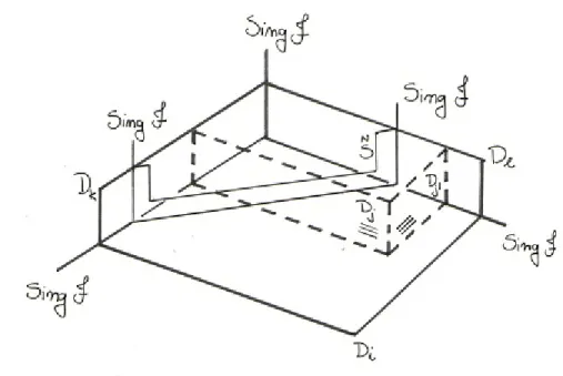
Figure 2: Example of arrangement of the irreducible components of the divisor.

Di, Dk, Dl are invariant components,Dj andDj0 are dicritical components and ˜S is

a convergent separatrix.

As in the two-dimensional case, we denote by ep(E) the number of irreducible

components of the normal crossings divisor E through p. We remark that in each intermediate ambient space Ms, the irreducible components of the divisor Es and

Ys (the center of πs+1) have normal crossings. We may write Es = Einvs ∪Edics as

before. Theorem 5 assures that for every point p∈ MN, we have that 1 ≤ τp ≤3,

0≤ep(EN)≤3 and the following inequality holds:

τp−1≤ep(EinvN )≤τp .

Hence if ep(EinvN ) = τp − 1, p is a trace point; and it is a corner in the case

ep(EinvN ) =τp.

The set σ_s−1(0) ⊂ Ms is a compact analytic subset that can be described as

(34)

and

σ−1_s (0) =π_s−1(σ−1_s₋₁(0)) .

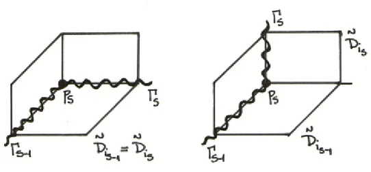
Moreover if Ys−1 ={p}is a point, we have that p∈σs−1−1(0) and thus Dss ⊂σs−1(0).

If Ys−1 is a curve, we have two possibilities:

a) Ys−1 is a compact curve, Ys−1 ⊂ σs−1−1(0). In this case Dss = πs−1(Ys−1) is a

compact divisor contained in σ−1_s (0).

b)Ys−1 is a germ of curve at a single point Ys−1∩σs−1−1(0) =q. In this caseπs−1(q)

is a compact curve contained in Ds

s and Dss is a germ of hypersurface around

π_s−1(q). In particularDs

s is a noncompact component of Es.

As we will see further, in this work we will never encounter possibility a).

1.9 The argument of Cano-Cerveau

In [5], F. Cano and D. Cerveau exhibit a method for constructing an invariant germ of surface once you have a reduction of singularities as in Theorem 5 and Remark 7. It essentially says that, if there are no dicritical components in the exceptional divisor EN _⊂_M

N, it is possible to continue each germ of invariant surface that rests

on a curve of the singular locus whose points are trace singularities of dimensional type two and thus construct, by projection, an invariant germ of surface at the origin 0∈_C3_.

The main result of [5] is the following

Theorem 6 (Existence of separatrices in dimension three) If F is a germ of holo-morphic singular foliation of codimension one over (_C3_,₀₎_{given by} _ω _{= 0} _{then one} of the following properties are satisfied:

(i) F has a germ of invariant surface.

(ii) There is an analytic mapping σ : (_C2_,₀₎ _→₍

C3,0) such that σ∗ω is not

iden-tically zero and the foliation given by σ∗ω = 0 has infinitely many analytic solutions through the origin.

We shall give here a brief description of Cano-Cerveau’s argument. Suppose F

does not fulfill (ii). Then after the reduction of singularities we do not encounter dicritical irreducible components inEN _⊂_M

N that project onto the origin (compact

(35)

Tr Sing FN =U {Y; Y is an irreducible component of Sing FN

which is generically contained in only one irre-ducible component of EN}.

Thus Tr Sing FN is a union of curves such that generically, every point of each

curve is a trace singularity of dimensional type two. Furthermore, it is clear that each Y ⊂ Tr Sing FN has normal crossings with EN and satisfies the following

properties:

−Y is not a singular curve;

− Either Y ⊂ π−1(0) and in this case it is a global compact curve; or

Y ∩π−1(0) =pY is one point and Y is a germ at pY, in which caseπ(Y)

is a germ of curve at the origin 0∈_C3_;

− IfY 6=Y0, then either Y ∩Y0 =∅or Y ∩Y0 =pY,Y0 is a single point.

Let Γ be a connected component of Tr Sing FN: Γ = Y1 ∪Y2 ∪ · · · ∪Yl where

the generical point of eachYi is a trace singularity of dimensional type two, and the

intersection points Yi∩Yj are trace singularities of dimensional type three. Then for

each point p∈Γ there exists a formal separatrix Sp; let us assume Sp is convergent.

By analytic triviality we may continue in an analytic way Sp to the points q ∈ Γ

such that eq(EinvN ) ≤ ep(EinvN ). The difficulty lies in continuing Sp to the points q0

where eq0(EN

inv) = 2, that is to say, to the points of Γ which are trace singularities

with dimensional type three. Nevertheless, it can also be done. Therefore we can “glue” the local separatrices Sp in order to obtain a closed hypersurface SΓ which gives, locally, a separatrix at each point of Γ. Due to the fact that the reduction of singularities (3) is a proper morphism, SΓ is projected to a convergent germ of separatrix S ⊂(_C3,0) of the foliation F.

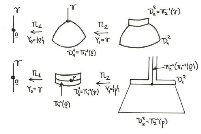
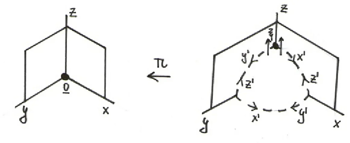
It remains to show that there is at least one connected component Γ of Tr Sing

FN that supports a convergent separatrix as above. Let ∆ be a non-degenerate

(36)

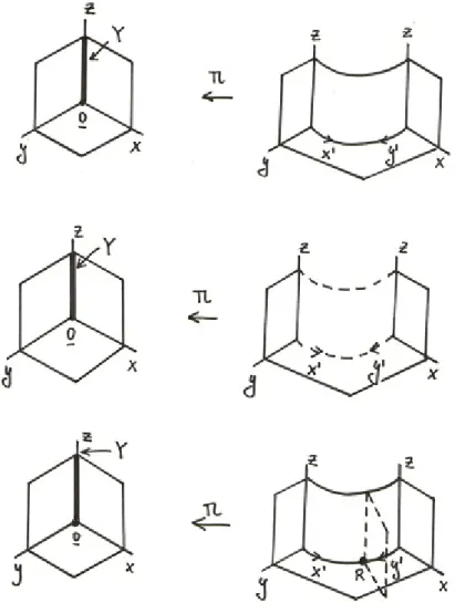
Figure 3: The argument of Cano-Cerveau

Lemma 9 [5] The strict transform of γ under the reduction of singularities of F,

γN = π∗γ, is nonsingular, not contained in Sing FN and transversal to EN at a

point p∈EN _{such that} _e

p(EinvN ) = 1.

With this lemma we conclude that the set Tr SingFN is not empty by showing

that the final transform ofγ intersectsEN at a pointpwhich is a trace singularity of dimensional type two; thus we find a curve contained in Tr SingFN passing through

it (see Figure 3).

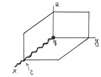
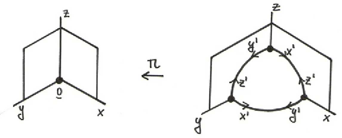
The presence of a compact dicritical component can prevent the extension process of constructing the separatrix S ⊂ (_C3_,_{0). For instance, in Jouanolou’s example} (see [12]), it is possible to construct a conic foliation F of (_C3,0) such that after a single blow-up centered at the origin we obtain only simple singularities, and the exceptional divisor - which only has one compact component - is generically transversal to the strict transform F0_{. Let} _G _{be a codimension one foliation of} (_C2_,_{0) with only simple singularities and which has no invariant curves. We may} build F so that the intersection of F0 _{and the exceptional divisor is precisely the} foliation G. SinceG has no invariant curves and F is a conic foliation of (_C3,0), we have that F has no invariant surfaces. The foliation F is given by the differential 1-form

(37)

Figure 4: Jouanolou’s example

This is the primary example of a holomorphic codimension one foliation in ambient space with dimension higher than two that has no invariant hypersurfaces.

However, there are other situations in which Cano-Cerveau’s argument works even if there are dicritical irreducible components in the exceptional divisor. For in-stance, if Sing F has codimension two, in ambient space dimension three this means that Sing F is a union of germs of curves at 0 ∈ _C3_{. If all dicritical irreducible} components generated during the reduction of singularities of F are projected onto these germs of curves, Cano-Cerveau’s argument is still valid. That is to say, if the dicritical components of the divisor are not compact, there is no risk of losing the compactness of the prolongation of the local invariant surfacesSp when intersecting

with these components, since the intersection of Sp and a dicritical component

re-sults in a germ of curve.

The argument is still valid when we have meromorphic first integrals in the compact dicritical components (see [23]).

1.10 Generic equireduction

(38)

analytic manifold M of dimension three (we will assume thatM is either compact or a germ over a compact set), a codimension one singular foliation F on M, and we also fix a normal crossings divisor E ⊂M.

We start by defining theadapted singular locus Sing(F, E) of F relatively toE. We recall that F and E havenormal crossings at a pointp∈M if and only ifF is nonsingular at p and

E∪H

defines a normal crossings divisor locally at p, where H is the only invariant hyper-surface of F through p. Then we define

Sing(F, E) = np∈M; F and E do not have normal crossings atpo .

By definition, we have that Sing F ⊂Sing (F, E). Moreover Sing(F, E) is a closed analytic subset of M of codimension at least two (to see this it is enough to remark that if F is tangent to a hypersurfaceD, then F and D have normal crossings at a generic point of D). Let us also remark that

Sing F = Sing(F,∅).

Before giving the precise definition ofpoint of equireduction, let us introduce the finite equireduction bamboos. Given a point p ∈ M, a finite equireduction bamboo for F, E of lengthN ≥0 over p is given by

B: n(Mk,Fk, Ek, Yk, pk;Uk)

oN

k=0 where we have the following properties:

1. Uk ik

,→Mk is an open subset of Mk, k = 0,1, . . . , N.

2. Yk ⊂Uk is a closed connected nonsingular curve having normal crossings with

Ek∩Uk, k = 0,1, . . . , N.

3. M0 = M and πk : Mk → Uk−1 is the blow-up with center Yk−1 for k = 1,2, . . . , N.

4. E0 =E and Ek =π_k−1(Yk−1∪(Ek−1 ∩Uk−1)) for k= 1,2, . . . , N. 5. p0 =pand πk(pk) = pk−1 for k = 1,2, . . . , N.

(39)

7. ik◦πk induces an ´etale morphism Yk →Yk−1 atpk.

Moreover, F0 = F, Fk is the transform by πk of Fk−1|_U_k−

1 and we add the conditions

8. Sing(Fk|Uk, E

k_∩_U

k) =Yk.

9. IfDk k =π

−1

k (Yk−1) is dicritical for Fk, we have one of the following properties:

a) (complete transversality) For each q∈Yk−1 the fiberπ_k−1(q) is generically transversal toFk.

b) (verticality) For each q∈Yk−1 the fiber π_k−1(q) is invariant byFk.

Remark 8 The existence of a finite equireduction bamboo of lengthN = 0 simply means that Sing (F, E) is a nonsingular curve at phaving normal crossings withE. Note that this property is satisfied at the generic points of the curves contained in Sing(F, E).

We can represent such a bamboo in a displayed way by the diagram

B: M ←i0- U0

π1

← M1

i1

←- U1

π2

← · · · πN

← MN

iN

←- UN

∪ ∪ ∪ ∪ ∪ ∪

E,F Y0 3p0 E1,F1 Y1 3p1 EN,FN YN 3pN

Definition 8 We say that a point p ∈ M is a point of equireduction for F, E if Sing(F, E) is a nonsingular curve at phaving normal crossings with E and for any finite equireduction bamboo

B: n(Mk,Fk, Ek, Yk, pk;Uk)

oN

k=0 there is an open set W ⊂UN, pN ∈W such that the blow-up

σ: ˜M →W

with center YN ∩W satisfies

1. IfE˜ =σ−1(YN∪(EN∩W))andF˜ is the transform ofFN byσ, then Sing( ˜F,E˜)

is a (possibly empty) union of nonsingular curves having normal crossings with ˜

E.

(40)

3. If σ is a dicritical blow-up, the we have either a) or b) where a) Each fiber σ−1(r) is generically transversal for r∈YN ∩W.

b) Each fiber σ−1(r), r∈YN ∩W, is invariant by F˜.

Remark 9 The bamboo B may be extended to several branches of length N + 1, except in the case that Sing( ˜F,E˜) = ∅. This case only occurs for a dicritical (completely transversal) morphism σ.

Letp∈M be a point with dimensional type τp = 2. So there exists a

neighbor-hood U ⊂M, p∈U, and a germ of nonsingular vector fieldξ inU which is tangent to F. Hence Sing(F, E)∩U is a nonsingular curve; moreover, it is contained in each invariant component of E∩U passing through p. If π:M0 →M is a blow-up centered at Y = Sing(F, E)∩U, we have that F1 is tangent to the vector field ξ1, the transform of ξ by π. Therefore, in the case that Sing(F1, E1)6= ∅, for any q ∈ Sing(F1, E1) we can find a neighborhood Uq ⊂ M1 such that Sing(F1, E1)∩Uq is

a nonsingular curve contained in each invariant component of E1_{. Repeating the} argument, we conclude that pis an equireduction point.

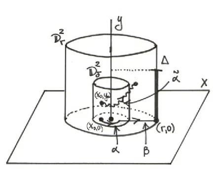
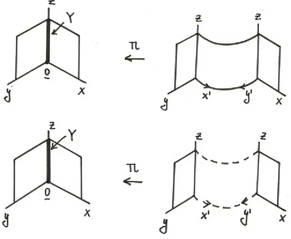
However, the properties “p ∈ M is an equireduction point for F, E” and “the dimensional type of p is two” are not equivalent. Take for instance M = (_C3_,_0),

E =∅ and F is the foliation given by ω = 0 where

ω =d[xy(x−y)(y+ (z+ 1)x)].

So Sing(F, E) = Sing F = (x=y= 0). By performing just one nondicritical blow-up π1 : M1 → M0 = M centered at Y0 = (x =y = 0), we obtain that every point of Sing(F1, E1) is simple. Note that Sing(F1, E1) is the union of four nonsingular curves which are locally isomorphic to Y0. If we continue performing blow-ups we will only obtain simple singularities. Hence every point p∈Sing(F, E) is an equire-duction point for F, E. However, note that the dimensional type of every pointp∈

Sing(F, E) is not two. Indeed, suppose we haveτp = 2. Then locally at pthe vector

field ξ = ∂/∂z is tangent to F. Hence F1 is (locally) tangent to the vector field

(41)

Figure 5: Equireduction is not equivalent to dimensional type two.

Let us state the main results on equireduction that we need in this work. The precise proofs may be found in [4], [8].

Proposition 10 Let p ∈ M be an equireduction point for F, E. Then there is an open set U ⊂M, p∈U, and a finite sequence of blow-ups

U π1

←− M1

π2

←− M2 ←− · · ·

πN

←− MN