Environmentally constrained null models: site suitability as occupancy criterion

(1)

OIKOS 93: 110 – 120. Copenhagen 2001

Environmentally constrained null models: site suitability as

occupancy criterion

Pedro R. Peres-Neto, Julian D. Olden and Donald A. Jackson

Peres-Neto, P. R., Olden, J. D. and Jackson, D. A. 2001. Environmentally con-strained null models: site suitability as occupancy criterion. – Oikos 93: 110 – 120.

Null models have proven to be an important quantitative tool in the search for ecological processes driving local diversity and species distribution. However, there remains an important concern that different processes, such as environmental condi-tions and biotic interaccondi-tions may produce similar patterns in species distribucondi-tions. In this paper we present an analytical protocol for incorporating habitat suitability as an occupancy criterion in null models. Our approach involves modeling species presence or absence as a function of environmental conditions, and using the estimated site-specific probabilities of occurrence as the likelihood of species occupancy of a site during the generation of ‘‘null communities’’. We validated this approach by showing that type I error is not affected by the use of probabilities as a site occupancy criterion and is robust against a variety of predictive performances of the species-en-vironmental models. We describe the expected differences when contrasting classical and the environmentally constrained null models, and illustrate our approach with a data set of Dutch dune hunting spider assemblages. An environmentally constrained approach to null models will provide a more robust evaluation of species associations by facilitating the distinction between mutually exclusive processes that may shape species distributions and community assembly.

P.R.Peres-Neto,J.D.Olden and D.A.Jackson,Dept of Zoology,Uni6.of Toronto,

Toronto, ON, Canada M5S 3G5 (pperes@zoo.utoronto.ca) (present address of JDO:

Dept of Biology,Colorado State Uni₆., Fort Collins,CO80523-1878,USA).

Null models have been used widely to investigate pat-terns in species distributions and to identify possible mechanisms (e.g., competition, predation) or assembly rules (e.g., limiting similarity, species saturation) re-stricting local community membership to subsets of the regional pool of potential colonizers (e.g., Caswell 1976, Connor and Simberloff 1979, Jackson et al. 1992, Cook and Quinn 1995, Gotelli and Graves 1996, Weiher and Keddy 1999). Null models constitute a body of statisti-cal methods to assess whether observed patterns in species distributions are distinct from arrangements of species taken at random from the regional pool. Con-ceptually, they are seen as quantitative tools for uncov-ering and testing conspicuous patterns in data rather than to elucidate the causal mechanisms responsible for such ecological patterns. For instance, nonrandom pat-terns in field data can serve as initial evidence for the

operation of particular ecological mechanisms shaping communities, which can subsequently be assessed ex-perimentally (e.g., Werner 1984, Juliano and Lawton 1990). Given that experimental data alone cannot ad-dress the extent to which particular local mechanisms are influential at macroecological scales (Maurer 1999), null models and experimentation are regarded as com-plementary tools in the search for mechanisms structur-ing ecological communities.

Null models of species distributions generally involve data of species incidence (i.e., presence or absence) across a number of patches, sites, local communities or islands. Frequencies of species co-occurrence are com-pared to expectations based on random site occupation to determine whether species exhibit non-random pat-terns in their distribution (Gotelli 2000). However, evi-dence for non-random patterns in species distributions

(2)

does not necessarily imply the role of biotic interac-tions, but could be equally related to other factors such as similarities or differences in dispersal abilities or environmental requirements of the species. In such cases, different processes like competition and environ-mental suitability could both lead to similar conclusions regarding patterns in species co-occurrences (i.e., rejec-tion of the null hypothesis; see Schluter 1984, Bradley and Bradley 1985 for discussions). We argue that our treatment of the biotic and abiotic factors as indepen-dent components is a practical one in the sense that patterns in species distribution may be more conspicu-ous when these components are independent (but see Brown et al. 2000, Stone et al. 2000). To maximize the chance of distinguishing among competing hypotheses, the likelihood of species co-occurrences should be as-sessed again after the environment is factored out as a possible explanation for the patterns encountered. The idea that ecological requirements of species should be incorporated into null models has been long recognized, yet is rarely addressed in the literature (Zobel 1997). Approaches to control for species habitat requirements in null models have taken different forms. The simplest approach fixes the total number of species per site and species frequencies (see Gotelli 2000) when generating the ‘‘null communities’’ in order to account for differ-ences in resource availability among sites and species-related characteristics. However, since species richness should vary with resource availability, this approach has been debated. Diamond and Marshall (1977) at-tempted to remove the effects of habitat diversity on species co-occurrences by using residuals from probit analysis to factor out differences in island sizes. Kelt et al. (1995) and Gotelli et al. (1997) incorporated geo-graphic and habitat characteristics directly into null models during the generation of ‘‘null communities’’ by assigning species to sites where they should be able to disperse naturally and persist.

In general, attempts made to incorporate environ-mental constraints into null models have been based on environmental classifications where habitats are grouped into categories (e.g., forest versus woodland, low versus high altitude). The fact that habitats cannot always be easily classified into discrete units (e.g., Knight and Morris 1996, Dufreˆne and Legendre 1997), promoting subjective classifications, and that species are more likely to exhibit a much finer response to habitat conditions, emphasizes the need to apply more quantitative approaches for incorporating habitat suit-ability into null models. The objective of our study is to present a novel approach for incorporating environ-mental constraints into null models. This approach involves modeling species presence or absence as a function of a set of environmental factors, and using the estimated site-specific probabilities of occurrence as the likelihood of species occupancy of a site during the generation of ‘‘null communities’’. After detailing the

protocol of the environmentally constrained null model approach, we conducted a simulation study to validate the model and described the expectations for the model. As an example, we used the approach with a data set of hunting spider assemblages from a Dutch dune area.

Unconstrained null models and co-occurrence

test statistics

A presence-absence matrix is the basis for the analysis of species distribution null models, where rows repre-sent species and columns reprerepre-sent sites or samples. Each matrix cell is coded (1) for presence and (0) for absence. To test whether the matrix contains non-ran-dom patterns of species co-occurrences, a rannon-ran-domiza- randomiza-tion test is used. The test begins by choosing a test statistic that reflects the question of interest and calcu-lating the measure for the original data. Next the observed test statistic is contrasted against a null distri-bution that is generated by randomly allocating the incidence values (1/0) in the matrix a large number of times (i.e., generate ‘‘null communities’’) and calculat-ing the test statistic for each randomized set. Under the null hypothesis the observed test statistic is just one possible value from the null distribution and its likeli-hood can be evaluated as the proportion of randomized values that are more extreme than the observed.

Perhaps the main source of disagreement among ecologists is the protocol that is used to generate the ‘‘null communities’’ (see Gotelli and Graves 1996 for a review). Although no consensus has been reached on the most appropriate protocol, ecologists have com-monly employed two algorithms for generating random matrices. The first randomizes the incidence values (1/0) fixing the sum of rows (i.e., species occurrences are maintained constant), whereas the second fixes the sum of both rows and columns (i.e., species occurrences and site richness are maintained constant). Depending on the algorithm, sites have different probabilities of being ‘‘randomly colonized’’; however all sites are assumed to provide similar environmental conditions because any of them could be successfully colonized by any species under chance alone. We refer to these approaches as unconstrained null models. Gotelli (2000) found that both provide appropriate type I error rates and com-parable statistical power.

(3)

indicate an increasing degree of mutual exclusivity be-tween species, where the maximum is reached when half of the sites are occupied by one species and the other occupies the other half. (2) The T-score statistic (Stone and Roberts 1992) calculates the degree of togetherness by counting the number of sites that species A and B jointly are either present or absent. A high T-score indicates common occurrence between species, where the maximum is achieved when half of the sites are occupied by both species and the other half lacks both species. (3) The S-score (Stone and Roberts 1992) mea-sures the number of shared sites occupied by both species A and B and is at its maximum when species occupy all sites. When conducting an analysis of the whole incidence matrix, C-, T- and S-scores are calcu-lated as the average from all species pairs.

Environmentally constrained null models

Figure 1 depicts the protocol for our environmentally constrained null model where two hypothetical species A and B were modeled according to two environmental

variables. The first step involves a single-species ap-proach to estimate the probability of species presence or absence at each study site based on the environmen-tal or habitat conditions. The resulting matrix contains site occurrence probabilities for each species at each site (i.e., site-specific probability matrix). A high predicted probability indicates that a site contains suitable envi-ronmental conditions for species occurrence, whereas a low probability suggests the lack of suitable environ-mental conditions. Predictions of site occurrence can be generated using a number of qualitative or quantitative approaches. For example, historical data could be used to assign probabilities of species colonization or infor-mation from experimental studies and field measures of habitat use could be used independently or combined to generate probabilities. An array of classification tech-niques such as discriminant analysis, logistic regression, classification trees, artificial neural networks or genetic algorithms is also available (see Hand 1997). In our hypothetical example (Fig. 1), we have used linear discriminant analysis to generate the species-specific probability matrix.

(4)

In the second step, probabilities of occurrence are transformed into relative probabilities, and species pres-ences are reassigned to sites during the generation of ‘‘null communities’’ according to these relative values (Fig. 1). We refer to this algorithm as Ct-RA1. In addition we consider situations where the probability of species occurrence is low (i.e., smaller than 0.5), al-though the species is observed present (i.e., poor predic-tion by the model). Using these probabilities during the generation of ‘‘null communities’’ would identify these sites as unfavorable although the species is present. Therefore, we propose a second algorithm Ct-RA2 that assigns a probability of 1.0 to all sites in the species-specific probability matrix where the species is actually present in the observed incidence matrix. Then proceed as for Ct-RA1, where probabilities are transformed into relative probabilities (Fig. 1). Therefore, for Ct-RA2 only the probabilities from the species-habitat models for empty sites are used. In both protocols we maintain fixed species frequencies, so that the number of sites occupied by any species in each random matrix is the same as in the observed matrix (Fig. 1). The con-strained randomization approach is then repeated a large number of times and at each time the index measuring species co-occurrence (Crnd, Trnd or Srnd) is

calculated and recorded. The observed value (Cobs, Tobs

or Sobs) is then contrasted to the null distribution of

random values and the probability of rejection is esti-mated (Fig. 1). The test is one-tailed and the probabil-ity is calculated as: (number of Crnd, Trndor Srndequal

to or larger than Cobs, Tobs or Sobs +1)/(number of

randomizations+1), where 1 represents the observed value for the index being evaluated and is also included as a value of the randomized distribution. For all analyses we used 1999 random permutations.

Validation of environmentally constrained

null models

Although the above protocol is ecologically sound, there is a need to verify whether the use of site-specific probabilities in null models could inflate or deflate the expected type I error rate (Roxburgh and Matsuki 1999, Peres-Neto and Olden 2001). To address this question we designed a Monte Carlo experiment (Manly 1997, Peres-Neto and Marques 2000) to vali-date empirically our constrained randomization al-gorithms. A sample-based Monte Carlo approach was employed because our interest relates to null models for distribution matrices that represent samples from a larger universe rather than complete censuses of species in island archipelagos.

The experiment involved generating a large number of random species incidence matrices. Empirical estima-tions of type I error were calculated as the proportion

(5)

Table 1. Summary of type I error estimates for unconstrained and constrained null models. Each entry is the proportion of tests for which the null hypothesis was rejected according to a specific alpha level when tested against a sample from a random incidence matrix. See text for details on the simulation protocols and null models used.

Unconstrained Environmentally constrained null models null models

Cr-RA2 Cr-RA1

Species-specific site probability matrix Species-specific site probability matrix

Alpha=0.10 1 2 3 4 1 2 3 4

C-score 0.108 0.115 0.112 0.109 0.127 0.093 0.086 0.075 0.107 T-score 0.106 0.135 0.110 0.108 0.132 0.100 0.089 0.085 0.108 S-score 0.093 0.126 0.099 0.090 0.128 0.091 0.085 0.096 0.098

Alpha=0.05

Alpha=0.01

correct classification success. We did not compare power since the unconstrained and constrained null models assess the likelihood of different alternative hypotheses. However, note that type I error compari-sons are justifiable as the null hypothesis is the same in both cases (i.e., absence of species association).

Environmentally constrained null models –

expectations

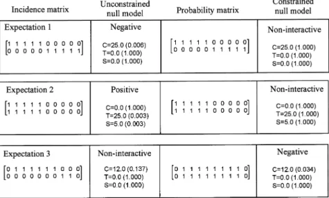
We anticipate three qualitative differences in interpreta-tions when contrasting the outcomes of unconstrained versus environmentally constrained null models. In Fig. 2 we provide a hypothetical example illustrating these expectations. Such expectations are due to the uncon-strained null model having a greater proportion of sites occupied as a result of chance alone relative to the constrained versions.

Expectation1 – The unconstrained null model detects a significant negative association between species (i.e., high C-score), whereas the constrained null model is non-significant (Fig. 2). In this case, negative associa-tions between species may be driven by the fact that they have different environmental requirements, so that biotic interactions between species are non-existent when species-environment relationships are taken into consideration.

Expectation2 – The unconstrained null model detects a significant positive association between species (i.e., high T- and S-scores), whereas the constrained null model is non-significant (Fig. 2). Here, positive

associa-tions between species can be explained by common species-environment affinities and not by biotic facilita-tion or similar dispersal capacities among species (Kelt et al. 1995). In these cases, species distributions overlap-ping in a relatively small fraction of sites should show the greatest differences between constrained and uncon-strained null models. In contrast, species with greater frequency of occurrence in the data and exhibiting positive associations may show no difference when environment is taken into account because the site-spe-cific probabilities will be closer to the actual percent of occurrence in the data set. Also, if one assumes that species with broad distributions are habitat generalists, environment should not be playing an important role in their distributions, so that in these cases both types of null models will likely provide similar outcomes.

(6)

rationale was that nearby quadrats should offer more similar environments than more distant ones.

We do not expect cases where the unconstrained null model is non-significant, but the constrained null model detects a positive association among species. Under the constrained permutation, a smaller number of sites is available to species and they will tend to co-occur more often under chance alone, decreasing the probability of rejection of positive associations. We also do not expect the case where the unconstrained null model detects a positive association between species and the constrained null model detects a negative association between spe-cies, or vice versa (but see Schoener and Adler 1991), because in our constrained null model only the proba-bility of the test statistic is affected (i.e., the observed test statistic is not changed). Cases where both con-strained and unconcon-strained null models agree in their outcomes imply that species interactions cannot be explained by environment alone. In the case of positive interactions, species occupying a smaller fraction of the available habitats, but overlapping highly in their distri-bution, may suggest facilitation. As discussed above in expectation 2, ubiquitous species also may not exhibit differences between the two types of null models. There is also the case where species may remain positively associated when they only overlap in fewer sites that offer a unique combination of environmental condi-tions, but not others.

Environmentally constrained null model in a

community of hunting spiders

Data were taken from ter Braak (1986: Table 3) and comprise the abundance values of 12 species of hunting spiders and environmental data for six habitat variables

from 28 sites (Table 2), originally presented by Van der Aart and Smeek-Enserink (1975). We constructed spe-cies-habitat models by modeling species presence-ab-sence as a function of six environmental characteristics using linear discriminant analysis. The results from the discriminant analyses produced a site-by-species matrix containing probability estimates for species occurrence of each site. A jackknife procedure (also called n-fold or leave-one-out cross validation) was used to validate the models because this approach provides a nearly unbiased estimate of prediction success (Olden and Jackson 2000). The jackknife approach excludes one site, constructs the models with the remaining 27 sites, and then predicts the probability of species occurrences for the excluded site using this model. This procedure is repeated 28 times so that each site, in turn, is excluded during the model construction and its response is pre-dicted. Overall correct classification rate was calculated as the percentage of sites where the model correctly predicted the presence or absence of a species and Cohen’s Kappa statistic was used to assess whether the model predictions differed from expectations based on chance alone (Titus et al. 1984). All single-species mod-els were found to be statistically significant (Table 3). To acquire a basic description of species-environmental affinities, we performed a principal component analysis (PCA) on correlations of the sites-by-species probability matrix so that each species could be compared in the reduced ordination space (Fig. 3). Arrows represent correlations between environmental variables and prin-cipal components. Our results largely agree with those presented by ter Braak (1986: Fig. 1) based on a canonical correspondence analysis.

Based on the entire incidence matrix, the unstrained null model and the two environmentally con-strained null models showed significant positive associations between species (C-score=30.2,P=1.000

(7)

(8)

Table 3. Results from discriminant analysis for predicting species presence-absence of hunting spider species based on environmental factors (see Table 2). Reported values are percentage of species occurrence (%SO), percentage of sites that the species was correctly classified (%CC), Kappa statistic and the associatedp-value (P). Species codes follow Table 2.

P

Species %SO %CC Kappa

AL 25.0 92.9 0.810 0.001

PL 60.7 96.4 0.926 0.001

ZS 60.7 92.9 0.850 0.001

PN 53.6 82.1 0.643 0.001

PP 46.4 92.9 0.855 0.001

AA 42.9 89.3 0.779 0.001

TT 92.9 96.4 0.650 0.007

AC 67.8 92.9 0.826 0.001

PM 75.0 96.4 0.909 0.001

AAc 60.7 96.4 0.926 0.001

AF 39.3 92.9 0.845 0.001

AP 21.4 92.9 0.818 0.001

Table 4. Summary of the null models results for the hunting spider data. Number of rejections for species pair-wise com-parisons for different significance levels is presented. For instance, for an alpha=0.05, 13 species pairs were negatively associated (C-score) according to the unconstrained null model.

Environmentally constrained Unconstrained

null models null models

Cr-RA2

C-score Cr-RA1

0

5 0

0.01

0 0

13 0.05

0.10 13 1 1

T-score

15 1 1

0.01

18 4 4

0.05

20

0.10 10 11

S-score

0.01 14 1 1

0.05 17 3 3

9 18

0.10 11

for all null models; T-score=54.8, PB0.0005 for all null models; S-score=8.9,PB0.0005 for all null mod-els). Examining species-pair associations showed that the number of significant interactions (both positive and negative) was much smaller for the environmen-tally constrained null model compared to the un-constrained (Table 4). Although there were a large number of negative interactions (Tables 4, 5), the mod-els based on the complete incidence matrix were not effective in detecting these associations, suggesting that when there are both positive and negative interactions between species, these indices may provide different power. Note that only three species had negative associ-ations, whereas six species had positive associations (Table 5).

Discussion

Our study describes a null-model protocol where spe-cies-environment associations can be accounted for when examining patterns in species incidence. The clas-sical approach (i.e., unconstrained) assumes that the environment is homogeneous across the landscape and thus unimportant in shaping species distributions, whereas the constrained approach incorporates species-specific responses to the environment. Therefore, the constrained approach facilitates a better evaluation of

(9)

the possible roles of biotic and abiotic factors shaping community structure. The comparison between classical null models and the constrained approach should provide the necessary contrast to judge which factor predominates. However, it is important to reiterate that the general value of null models based on distributional data is in verifying patterns related to similar or com-plementary distributions, rather than asserting that cer-tain mechanisms are important or unimportant. For instance, because species that compete may be more likely to share similar habitats, positive associations are also expected under strong competition (Schluter 1984, Kelt and Brown 1999). The value of our analytical approach is not different in this regard; however, it addresses the question of whether or not associations between species may be simply ascribed to environmen-tal affinities, rather than biotic interactions, and also tests whether species have more similar or distinct habitat requirements.

The results show that accounting for environmental suitability of the dune sites greatly influences the inter-pretation of interactions between hunting spider species as we found that differences or similarities in species environmental requirements largely described the pat-terns of association between species (Tables 4, 5). Con-sequently, this removed the need to invoke facilitation or competition as plausible mechanisms determining most species distributions. For instance,A.pericolaand P. lugrubisare negatively associated based on the re-sults from the unconstrained null model; however, they have very different environmental affinities for the amount of bare sand, cover moss and water content (Fig. 3), thus resulting in no significant association according to the constrained null model. In contrast,A. albimana andA. lutetianaare positively associated ac-cording to the unconstrained null model, but are ran-domly associated in the environmentally constrained null models because these species were found at sites with very similar environmental conditions (Fig. 3). Interestingly, A. cuneata and P. nigriceps remained

positively associated after the environment was incor-porated (Table 5). Although these two species exhibit somewhat different environmental preferences (Fig. 3), they frequently overlap at sites having the combination of few fallen twigs but high light reflectivity (Table 2), suggesting an interaction of these two variables in facilitating coexistence. Associations that remain signifi-cant after accounting for species-environment relation-ships may be related to three aspects: (1) species associations are truly related to biotic interactions; (2) interactions between some environmental factors at particular sites might facilitate coexistence; and (3) important environmental variables not used in the spe-cies-environment models may contribute to their joint or disjoint distribution. Regardless, our null model will be effective in revealing those associations that can be explained by the measured environmental variables from those that cannot be explained.

A number of conditions may decouple species-habi-tat relationships and introduce errors into species-envi-ronmental models. For instance, some sites may provide environmental conditions suitable for persis-tence; however, dispersal barriers may impede immigra-tion into the site (e.g., Lonzarich et al. 1998). Competitive interactions may also displace species from their optimum into sub-optimal habitats in a number of sites. An interesting extension to the constrained ap-proach would be to sample site-specific probabilities within confidence intervals for site probabilities (see Taylor 1991) at each randomization so that the degree of error would be also incorporated into the null model. In the worst-case scenario, where species models present extremely high degrees of errors, the uncon-strained and conuncon-strained null models would provide equivalent outcomes (Peres-Neto unpubl.).

By fixing species frequencies in our null models, we assumed that the probability of random colonization of sites is a function of the fraction of sites occupied. However, species frequencies are also an important outcome of competitive interactions, and perhaps may

Table 5. Pair-wise associations between hunting spiders. Positive associations (+) were assessed by the significance of the T-score (note: S-score provided similar results). Negative associations (−) were judged by the significance of the C-score. All results based on alpha=0.05. The upper diagonal contains the results based on the unconstrained null model, whereas the lower diagonal has the results for Cr-RA1 (note: Cr-RA2 provided similar results). Species codes follow Table 2.

AL PL ZS PN PP AA TT AC PM AAc AF AP

AL + + + + +

+

PL − − −

ZS + + + + − − −

+ + +

PN − −

+ + + −

PP

+ + + −

AA

−

TT

+ + − −

AC +

(10)

also reflect positive associations (Gotelli 2000 and refer-ences therein). As a consequence, fixing species frequen-cies may incorporate the outcomes from previous species interactions into the ‘‘null communities’’, lower-ing the power of detectlower-ing true associations. Relaxlower-ing this assumption may provide important insights. For instance, some components of metapopulation or bio-geographic models may be adapted and incorporated into constrained null models for predicting site occu-pancy, as well as generating random site occupancy via simple stochastic processes (e.g., Haydon et al. 1993, Hanski 1994). The use of more complex species-envi-ronmental models for predicting species incidence may be modified to incorporate aspects related to spatial location of sites (Roxburgh and Matsuki 1999) such as isolation, connectivity and corridor quality and species dispersal abilities into null models.

Our study has detailed methods for incorporating site-specific probabilities into null models so that spe-cies selected to compose ‘‘null communities’’ could occupy the environment offered by randomly selected sites under normal conditions rather than occurrences simply being mediated by species interactions. Given the vast number of data sets containing data on species distributions and site environmental conditions, the method presented here should facilitate a more robust evaluation of the factors contributing to species associ-ations and community organization.

Acknowledgements– We would like to thank Nicholas Gotelli for stimulating discussions regarding null models and helpful comments on this paper and Bryan Manly for his insights regarding Monte Carlo simulations for type I error estimation. Funding for this project was provided by a CNPq Fellowship to PRP-N, a Natural Sciences and Engineering Research Council of Canada (NSERC) Graduate Scholarship to JDO and an NSERC Research grant to DAJ. A computer program to carry out the null model protocols presented here is avail-able on_Bhttp://www.zoo.utoronto.ca/jackson/software/_\.

References

Bradley, R. A. and Bradley, D. W. 1985. Do non-random patterns of species in niche space imply competition? – Oikos 45: 443 – 446.

Brown, J. H., Fox, B. J. and Kelt, D. A. 2000. Assembly rules: desert rodent communities are structured at scales from local to continental. – Am. Nat. 156: 314 – 321.

Caswell, H. 1976. Community structure: a neutral model analysis. – Ecol. Monogr. 46: 327 – 354.

Connor, E. F. and Simberloff, D. 1979. The assembly of species communities: chance or competition? – Ecology 60: 1132 – 1140.

Cook, R. and Quinn, J. F. 1995. The importance of coloniza-tion in nested species subsets. – Oecologia 102: 413 – 424. Diamond, J. M. and Marshall, A. G. 1977. Distributional

ecology of New Hebridian birds: a species keleidoscope. – J. Anim. Ecol. 46: 703 – 727.

Dufreˆne, M. and Legendre, P. 1997. Species assemblages and indicator species: the need for a flexible asymmetrical ap-proach. – Ecol. Monogr. 67: 345 – 366.

Gotelli, N. J. 2000. Null model analysis of species co-occur-rence patterns. – Ecology 81: 2606 – 2621.

Gotelli, N. J. and Graves, G. R. 1996. Null models in ecology. – Smithsonian Inst. Press.

Gotelli, N. J., Buckley, N. J. and Wiens, J. A. 1997. Co-occur-rence of Australian birds: Diamond’s assembly rules revis-ited. – Oikos 80: 311 – 324.

Hand, D. J. 1997. Construction and assessment of classifica-tion rules. – John Wiley and Sons.

Hanski, I. 1994. A practical model of metapopulation dynam-ics. – J. Anim. Ecol. 63: 151 – 162.

Haydon, D., Radtkey, R. R. and Pianka, E. R. 1993. Experi-mental biogeography: interactions between stochastic, his-torical, and ecological processes in a model archipelago. – In: Ricklefs, R. E. and Schluter, D. (eds), Species diversity in ecological communities – historical and geographical perspectives. Univ. of Chicago Press, pp. 117 – 130. Jackson, D. A., Somers, K. M. and Harvey, H. H. 1989.

Similarity coefficients: measures of co-occurrence and asso-ciation or simply measures of occurrence. – Am. Nat. 133: 436 – 453.

Jackson, D. A., Somers, K. M. and Harvey, H. H. 1992. Null models and fish communities: evidence of nonrandom pat-terns. – Am. Nat. 139: 930 – 951.

Jason, S. and Vegelius, J. 1981. Measures of ecological associ-ation. – Oecologia 49: 371 – 376.

Juliano, S. A. and Lawton, J. H. 1990. The relationship between competition and morphology. II. Experiments on co-occurring dystiscid beetles. – J. Anim. Ecol. 59: 831 – 848.

Kelt, D. A. and Brown, J. H. 1999. Community structure and assembly rules: confronting conceptual and statistical is-sues with data on desert rodents. – In: Weiher, E. and Keddy, P. (eds), Ecological assembly rules: perspectives, advances, retreats. Cambridge Univ. Press, pp. 75 – 107. Kelt, D. A., Taper, M. L. and Meserve, P. L. 1995. Assessing

the impact of competition on community assembly: a case study using small mammals. – Ecology 76: 1283 – 1296. Knight, T. W. and Morris, D. W. 1996. How many habitats

do landscapes contain? – Ecology 77: 1756 – 1764. Lonzarich, D. G., Warren, M. L. and Conzarich, M. E. 1998.

Effects of habitat isolation on the recovery of fish assem-blages in experimentally defaunated stream pools in Ar-kansas. – Can. J. Fish. Aquat. Sci. 55: 2141 – 2149. Manly, B. J. F. 1997. Randomization, bootstrap and Monte

Carlo methods in biology. – Chapman and Hall. Maurer, B. A. 1999. Untangling ecological complexity: the

macroscopic perspective. – Univ. of Chicago Press. Olden, J. D. and Jackson, D. A. 2000. Torturing data for the

sake of generality: how valid are our regression models. – E´ coscience 7 (in press).

Peres-Neto, P. R. and Marques, F. 2000. When are random data not random, or is the PTP test useful? – Cladistics (in press).

Peres-Neto, P. R. and Olden, J. D. 2001. Assessing the robust-ness of randomization tests: examples from behavioural studies. – Anim. Behav. (in press).

Roxburgh, S. H. and Matsuki, M. 1999. The statistical valida-tion of null models used in spatial associavalida-tion analysis. – Oikos 85: 68 – 78.

Schluter, D. A. 1984. A variance test for detecting species associations, with some example applications. – Ecology 65: 998 – 1005.

Schoener, T. W. and Adler, G. H. 1991. Greater resolution of distributional complementarities by controlling for habitat affinities: a study with Bahamian lizards and birds. – Am. Nat. 137: 669 – 692.

Stone, L. and Roberts, A. 1992. Competitive exclusion, or species aggregation? An aid in deciding. – Oecologia 91: 419 – 424.

(11)

Taylor, B. 1991. Investigating species incidence over habitat fragmentation of different areas – a look at error estima-tion. – In: Gilpin, M. and Hanski, I. (eds), Metapopula-tion dynamics: empirical and theoretical investigaMetapopula-tions. Academic Press, pp. 177 – 191.

ter Braak, C. J. F. 1986. Canonical correspondence analysis: a new eigenvector technique for multivariate direct gradient analysis. – Ecology 67: 1167 – 1179.

Titus, K., Mosher, J. A. and Williams, B. K. 1984. Chance-corrected classification for use in discriminant analysis: ecological applications. – Am. Midl. Nat. 111: 1 – 7. Van der Aart, P. J. and Smeek-Enserink, N. 1975. Correlation

between distributions of hunting spiders (Lycosidae, Ctenidae) and environmental characteristics in a dune area. – Neth. J. Zool. 25: 1 – 45.

Weiher, E. and Keddy, P. 1999. Introduction: the scope and goals of research on assembly rules. – In: Weiher, E. and Keddy, P. (eds), Ecological assembly rules: perspectives, advances, retreats. Cambridge Univ. Press, pp. 1 – 20. Werner, E. E. 1984. The mechanisms of species interactions

and community organization in fish. – In: Strong, D. R., Jr., Simberloff, D., Abele, L. G. and Thistle, A. B. (eds), Ecological communities: conceptual issues and evidence. Princeton Univ. Press, pp. 360 – 382.

Wilson, J. B. and Gitay, H. 1995. Limitations to species coexistence: evidence for competition from field observa-tions, using a patch model. – J. Veg. Sci. 6: 369 – 376. Zobel, M. 1997. The relative role of species pools in