Advanced Probability Theory
for Biomedical Engineers
John D. Enderle, David C. Farden, and Daniel J. Krause www.morganclaypool.com
ISBN-10: 1598291505 paperback ISBN-13: 9781598291506 paperback ISBN-10: 1598291513 ebook ISBN-13: 9781598291513 ebook
DOI 10.2200/S00063ED1V01Y200610BME011 A lecture in the Morgan & Claypool Synthesis Series
SYNTHESIS LECTURES ON BIOMEDICAL ENGINEERING #11
Lecture #11
Series Editor: John D. Enderle, University of Connecticut
Series ISSN: 1930-0328 print Series ISSN: 1930-0336 electronic First Edition
Advanced Probability Theory
for Biomedical Engineers
John D. Enderle
Program Director & Professor for Biomedical Engineering, University of Connecticut
David C. Farden
Professor of Electrical and Computer Engineering, North Dakota State University
Daniel J. Krause
Emeritus Professor of Electrical and Computer Engineering, North Dakota State University
SYNTHESIS LECTURES ON BIOMEDICAL ENGINEERING #11
M
&
C
M or g a n
&
C l ay p o ol P u b l i s h e r s
ABSTRACT
This is the third in a series of short books on probability theory and random processes for biomedical engineers. This book focuses on standard probability distributions commonly en-countered in biomedical engineering. The exponential, Poisson and Gaussian distributions are introduced, as well as important approximations to the Bernoulli PMF and Gaussian CDF. Many important properties of jointly Gaussian random variables are presented. The primary subjects of the final chapter are methods for determining the probability distribution of a func-tion of a random variable. We first evaluate the probability distribufunc-tion of a funcfunc-tion of one random variable using the CDF and then the PDF. Next, the probability distribution for a single random variable is determined from a function of two random variables using the CDF. Then, the joint probability distribution is found from a function of two random variables using the joint PDF and the CDF.
The aim of all three books is as an introduction to probability theory. The audience includes students, engineers and researchers presenting applications of this theory to a wide variety of problems—as well as pursuing these topics at a more advanced level. The theory material is presented in a logical manner—developing special mathematical skills as needed. The mathematical background required of the reader is basic knowledge of differential calculus. Pertinent biomedical engineering examples are throughout the text. Drill problems, straight-forward exercises designed to reinforce concepts and develop problem solution skills, follow most sections.
KEYWORDS
Contents
5. Standard Probability Distributions . . . 1
5.1 Uniform Distributions . . . 1
5.2 Exponential Distributions . . . 4
5.3 Bernoulli Trials . . . 6
5.3.1 Poisson Approximation to Bernoulli . . . 11
5.3.2 Gaussian Approximation to Bernoulli . . . 12
5.4 Poisson Distribution . . . 14
5.4.1 Interarrival Times . . . 18
5.5 Univariate Gaussian Distribution . . . 20
5.5.1 Marcum’s Q Function . . . 25
5.6 Bivariate Gaussian Random Variables . . . 26
5.6.1 Constant Contours. . . .32
5.7 Summary . . . 36
5.8 Problems . . . 36
6. Transformations of Random Variables . . . 45
6.1 Univariate CDF Technique . . . 45
6.1.1 CDF Technique with Monotonic Functions . . . 45
6.1.2 CDF Technique with Arbitrary Functions . . . 46
6.2 Univariate PDF Technique . . . 53
6.2.1 Continuous Random Variable . . . 53
6.2.2 Mixed Random Variable . . . 56
6.2.3 Conditional PDF Technique . . . 57
6.3 One Function of Two Random Variables . . . 59
6.4 Bivariate Transformations . . . 63
6.4.1 Bivariate CDF Technique . . . 63
6.4.2 Bivariate PDF Technique . . . 65
6.5 Summary . . . 73
Preface
This is the third in a series of short books on probability theory and random processes for biomedical engineers. This text is written as an introduction to probability theory. The goal was to prepare students at the sophomore, junior or senior level for the application of this theory to a wide variety of problems - as well as pursue these topics at a more advanced level. Our approach is to present a unified treatment of the subject. There are only a few key concepts involved in the basic theory of probability theory. These key concepts are all presented in the first chapter. The second chapter introduces the topic of random variables. The third chapter focuses on expectation, standard deviation, moments, and the characteristic function. In addition, conditional expectation, conditional moments and the conditional characteristic function are also discussed. The fourth chapter introduces jointly distributed random variables, along with joint expectation, joint moments, and the joint characteristic function. Convolution is also developed. Later chapters simply expand upon these key ideas and extend the range of application.
This short book focuses on standard probability distributions commonly encountered in biomedical engineering. Here in Chapter 5, the exponential, Poisson and Gaussian distributions are introduced, as well as important approximations to the Bernoulli PMF and Gaussian CDF. Many important properties of jointly distributed Gaussian random variables are presented. The primary subjects of Chapter 6 are methods for determining the probability distribution of a function of a random variable. We first evaluate the probability distribution of a function of one random variable using the CDF and then the PDF. Next, the probability distribution for a single random variable is determined from a function of two random variables using the CDF. Then, the joint probability distribution is found from a function of two random variables using the joint PDF and the CDF.
A considerable effort has been made to develop the theory in a logical manner - developing special mathematical skills as needed. The mathematical background required of the reader is basic knowledge of differential calculus. Every effort has been made to be consistent with commonly used notation and terminology—both within the engineering community as well as the probability and statistics literature.
and biomedical phenomena. However, we do introduce some pertinent biomedical engineering examples throughout the text.
Students in other fields should also find the approach useful. Drill problems, straightfor-ward exercises designed to reinforce concepts and develop problem solution skills, follow most sections. The answers to the drill problems follow the problem statement in random order. At the end of each chapter is a wide selection of problems, ranging from simple to difficult, presented in the same general order as covered in the textbook.
C H A P T E R 5
Standard Probability Distributions
A surprisingly small number of probability distributions describe many natural probabilistic phenomena. This chapter presents some of these discrete and continuous probability distribu-tions that occur often enough in a variety of problems to deserve special mention. We will see that many random variables and their corresponding experiments have similar properties and can be described by the same probability distribution. Each section introduces a new PMF or PDF. Following this, the mean, variance, and characteristic function are found. Additionally, special properties are pointed out along with relationships among other probability distribu-tions. In some instances, the PMF or PDF is derived according to the characteristics of the experiment. Because of the vast number of probability distributions, we cannot possibly discuss them all here in this chapter.
5.1
UNIFORM DISTRIBUTIONS
Definition 5.1.1. The discrete RV x has a uniform distribution over n points (n>1) on the interval [a,b] if x is a lattice RV with span h =(b−a)/(n−1) and PMF
px(α)=
1/n, α=kh+a,k =0,1, . . . ,n−1
0, otherwise. (5.1)
The mean and variance of a discrete uniform RV are easily computed with the aid of Lemma 2.3.1:
ηx =
1 n
n−1
k=0
(kh+a)= h n
γ[2]
n
2 +a = 1 n
b−a n−1
n(n−1) 2 +a =
b+a
2 , (5.2)
and
σ2
x =
1 n
n−1
k=0
kh− b−a 2
2
= (b−a)2 n
n−1
k=0
k2 (n−1)2 −
k n−1 +
1 4 . (5.3) Simplifying, σ2 x =
(b−a)2 12
n+1
0 .5 1
x
p ( )
.05
(a)
1
x(t )
t
10 30 50 (b)
φ
α α
FIGURE 5.1: (a) PMF and (b) characteristic function magnitude for discrete RV with uniform distri-bution over 20 points on [0,1].
The characteristic function can be found using the sum of a geometric series:
φx(t)=
ejat
n
n−1
k=0
(ejht)k = e
jat
n
1−ejhnt
1−ejht . (5.5)
Simplifying with the aid of Euler’s identity,
φx(t)=exp
ja +b 2 t
sinb−a
2
n n−1t
n sinb−2an−11t. (5.6)
Figure 5.1 illustrates the PMF and the magnitude of the characteristic function for a discrete RV which is uniformly distributed over 20 points on [0,1]. The characteristic function is plotted over [0, π/h], where the span h =1/19. Recall from Section 3.3 thatφx(−t)=φx∗(t) and that
φx(t) is periodic in t with period 2π/h. Thus, Figure 5.1 illustrates one-half period of|φx(·)|.
Definition 5.1.2. The continuous RV x has a uniform distribution on the interval [a,b] if x has PDF
fx(α)=
1/(b−a), a ≤α ≤b
0, otherwise. (5.7)
The mean and variance of a continuous uniform RV are easily computed directly:
ηx =
1 b−a
b
a
αdα = b 2−a2
2(b−a) = b+a
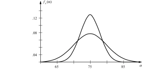
0 .5 1 1
(a)
1
x(t )
φ
t
10 30 50 (b)
x
f (α)
FIGURE 5.2: (a) PDF and (b) characteristic function magnitude for continuous RV with uniform distribution on [0,1].
and
σ2
x =
1 b−a
b
a
α−b+a
2 2
dα = (b−a) 2
12 . (5.9)
The characteristic function can be found as
φx(t)=
1 b−a
b
a
ejαtdα= exp
jb+2at b−a
(b−a)/2
−(b−a)/2 ejαtdα.
Simplifying with the aid of Euler’s identity,
φx(t)=exp
ja +b 2 t
sinb−2at
b−a
2 t
. (5.10)
Figure 5.2 illustrates the PDF and the magnitude of the characteristic function for a continuous RV uniformly distributed on [0,1]. Note that the characteristic function in this case is not periodic butφx(−t)=φx∗(t).
Drill Problem 5.1.1. A pentahedral die (with faces labeled 0,1,2,3,4) is tossed once. Let x be a
random variable equaling ten times the number tossed. Determine: (a) px (20), (b) P(10≤x ≤50),
(c) E(x), (d)σ2
x.
Answers: 20, 0.8, 200, 0.2.
Drill Problem 5.1.2. Random variable x is uniformly distributed on the interval [−1,5]. Deter-mine: (a) Fx (0), (b) Fx(5),(c)ηx, (d)σx2.
5.2
EXPONENTIAL DISTRIBUTIONS
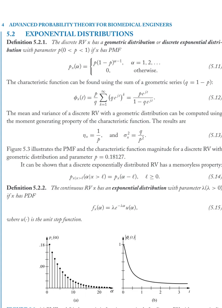
Definition 5.2.1. The discrete RV x has a geometric distribution or discrete exponential
distri-bution with parameter p(0< p<1) if x has PMF
px(α)=
p(1−p)α−1, α=1,2, . . .
0, otherwise. (5.11)
The characteristic function can be found using the sum of a geometric series (q =1−p):
φx(t)=
p q
∞
k=1
q ej tk = pe
j t
1−q ej t. (5.12)
The mean and variance of a discrete RV with a geometric distribution can be computed using the moment generating property of the characteristic function. The results are
ηx =
1
p, and σ 2
x =
q
p2. (5.13)
Figure 5.3 illustrates the PMF and the characteristic function magnitude for a discrete RV with geometric distribution and parameter p=0.18127.
It can be shown that a discrete exponentially distributed RV has a memoryless property:
px|x>(α|x > )= px(α−), ≥0. (5.14)
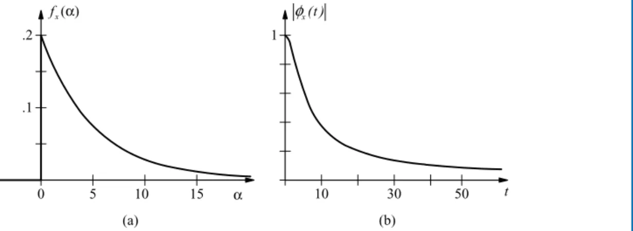
Definition 5.2.2. The continuous RV x has an exponential distribution with parameterλ(λ >0) if x has PDF
fx(α)=λe−λαu(α), (5.15)
where u(·) is the unit step function.
0 10 20 α
x
p (α) .18
.09
(a)
1
x(t )
φ
t
0 1 2 3 (b)
0 5 10 .2
x
f (α)
.1
1
x(t )
φ
t
10 30 50
(a) (b)
15 α
FIGURE 5.4: (a) PDF and (b) characteristic function magnitude for continuous RV with exponential distribution and parameterλ=0.2.
The exponential probability distribution is also a very important probability density function in biomedical engineering applications, arising in situations involving reliability theory and queuing problems. Reliability theory, which describes the time to failure for a system or compo-nent, grew primarily out of military applications and experiences with multicomponent systems. Queuing theory describes the waiting times between events.
The characteristic function can be found as
φx(t)=λ
∞
0
eα( j t−λ)dα= λ
λ− j t. (5.16)
Figure 5.4 illustrates the PDF and the magnitude of the characteristic function for a continuous RV with exponential distribution and parameterλ=0.2.
The mean and variance of a continuous exponentially distributed RV can be obtained using the moment generating property of the characteristic function. The results are
ηx =
1
λ, σx2 =
1
λ2. (5.17)
A continuous exponentially distributed RV, like its discrete counterpart, satisfies a memoryless property:
fx|x>τ(α|x> τ)= fx(α−τ), τ ≥0. (5.18)
Example 5.2.1. Suppose a system contains a component that has an exponential failure rate.
Solution. First, the parameterλis determined from
0.95= P (x>5000)=
∞
5000
λe−λαdα=e−5000λ.
Thus
λ= −ln(0.95)
5000 =1.03×10
−5.
Then, to determine the number of hours reliable at 99%, we solve forαfrom
P (x> α)=e−λα=0.99
or
α = −ln(0.99)λ =980 hours.
Drill Problem 5.2.1. Suppose a system has an exponential failure rate in years to failure with
λ=0.02. Determine the number of years reliable at: (a) 90%, (b) 95%, (c) 99%.
Answers: 0.5, 2.6, 5.3.
Drill Problem 5.2.2. Random variable x, representing the length of time in hours to complete an
examination in Introduction to Random Processes, has PDF
fx(α)=
4 3e
−43αu(α).
The examination results are given by
g (x)=
⎧ ⎪ ⎨ ⎪ ⎩
75, 0<x<4/3 75+39.44(x−4/3), x≥4/3
0, otherwise.
Determine the average examination grade.
Answer: 80.
5.3
BERNOULLI TRIALS
bit, or an even and odd number in a die toss. Let us call one of the events a success, the other a failure. The Bernoulli PMF describes the probability of k successes in n trials of a Bernoulli experiment. The first two chapters used this PMF repeatedly in problems dealing with games of chance and in situations where there were only two possible outcomes in any given trial. For biomedical engineers, the Bernoulli distribution is used in infectious disease problems and other applications. The Bernoulli distribution is also known as a Binomial distribution.
Definition 5.3.1. A discrete RV x is Bernoulli distributed if the PMF for x is
px(k)=
⎧ ⎪ ⎨ ⎪ ⎩
n k
pkqn−k, k =0,1, . . . ,n
0, otherwise,
(5.19)
where p =probability of success and q =1−p.
The characteristic function can be found using the binomial theorem:
φx(t)= n
k=0
n k
( pej t)kqn−k =(q +pej t)n. (5.20)
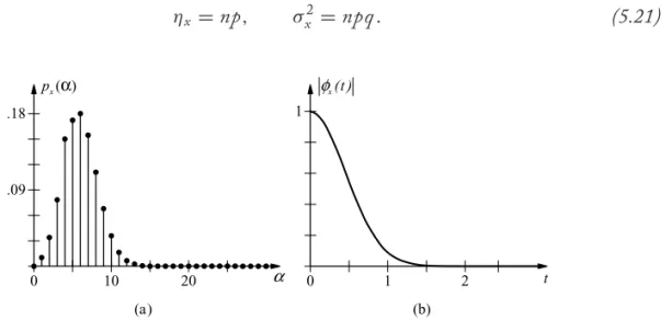
Figure 5.5 illustrates the PMF and the characteristic function magnitude for a discrete RV with Bernoulli distribution, p =0.2, and n=30.
Using the moment generating property of characteristic functions, the mean and variance of a Bernoulli RV can be shown to be
ηx =np, σx2=npq. (5.21)
0 10 20 α
x
p (α) .18
.09
(a)
1
x(t )
φ
t
0 1 2
(b)
Unlike the preceding distributions, a closed form expression for the Bernoulli CDF is not easily obtained. Tables A.1–A.3 in the Appendix list values of the Bernoulli CDF for p = 0.05,0.1,0.15, . . . ,0.5 and n=5,10,15, and 20. Let k∈ {0,1, . . . ,n−1}and define
G(n,k,p)=
k
=0
n
p(1−p)n−.
Making the change of variable m =n−yields
G(n,k,p)=
n
m=n−k
n n−m
pn−m(1−p)m.
Now, since
n n−m
= n!
m! (n−m)! =
n m
,
G(n,k,p)=
n
m=0
n m
pn−m(1−p)m−
n−k−1
m=0
n m
pn−m(1−p)m.
Using the Binomial Theorem,
G(n,k,p)=1−G(n,n−k−1,1−p). (5.22)
This result is easily applied to obtain values of the Bernoulli CDF for values of p >0.5 from Tables A.1–A.3.
Example 5.3.1. The probability that Fargo Polytechnic Institute wins a game is 0.7. In a 15 game
season, what is the probability that they win: (a) at least 10 games, (b) from 9 to 12 games, (c) exactly 11 games? (d) With x denoting the number of games won, findηx andσx2.
Solution. With x a Bernoulli random variable, we consult Table A.2, using (5.22) with n=15, k =9, and p =0.7, we find
a) P (x ≥10)=1−Fx(9)=1.0−0.2784=0.7216,
b) P (9≤x ≤12)= Fx(12)−Fx(8)=0.8732−0.1311=0.7421,
c) px(11)= Fx(11)−Fx(10)=0.7031−0.4845=0.2186.
We now consider the number of trials needed for k successes in a sequence of Bernoulli trials. Let
p(k,n)= P (k successes in n trials) (5.23)
= ⎧ ⎪ ⎨ ⎪ ⎩
n k
pkqn−k, k =0,1, . . . ,n
0, otherwise,
where p = p(1,1) and q =1− p. Let RV nr represent the number of trials to obtain exactly
r successes (r ≥1). Note that
P (success inth trial|r −1 successes in previous−1 trials)= p; (5.24)
hence, for=r,r +1, . . ., we have
P (nr =)= p(r −1, −1) p. (5.25)
Discrete RV nr thus has PMF
pnr()= ⎧ ⎪ ⎨ ⎪ ⎩
−1
r−1
prq−r, =r,r+1, . . .
0, otherwise,
(5.26)
where the parameter r is a positive integer. The PMF for the RV nr is called the negative
binomial distribution, also known as the P´olya and the Pascal distribution. Note that with
r =1 the negative binomial PMF is the geometric PMF.
The moment generating function for nr can be expressed as
Mnr(λ)=
∞
=r
(−1)(−2)· · ·(−r +1)
(r−1)! p
rq−reλ.
Letting m =−r , we obtain
Mnr(λ)= eλrpr
(r −1)!
∞
m=0
(m+r−1)(m+r −2)· · ·(m+1)(q eλ)m.
With
s (x)=
∞
k=0
xk = 1
we have
s()(x) =
∞
k=
k(k−1)· · ·(k−+1)xk−
=∞
m=0
(m+)(m+−1)· · ·(m+1)xm
= !
(1−x)+1.
Hence
Mnr(λ)=
peλ 1−q eλ
r
, q eλ<1. (5.27)
The mean and variance for nr are found to be
ηnr = r
p, and σ 2
nr = r q
p2. (5.28)
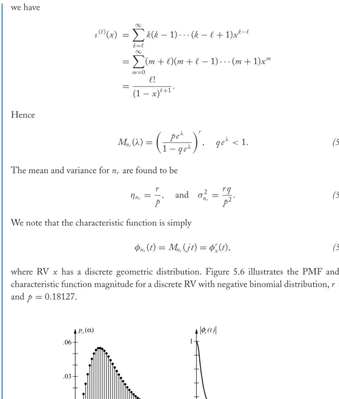
We note that the characteristic function is simply
φnr(t)=Mnr( j t)=φ
r
x(t), (5.29)
where RV x has a discrete geometric distribution. Figure 5.6 illustrates the PMF and the characteristic function magnitude for a discrete RV with negative binomial distribution, r =3, and p =0.18127.
1
x(t )
φ
t
0 1 2
(b) 0 20 40 α
x
p (α) .06
.03
(a)
5.3.1 Poisson Approximation to Bernoulli
When n becomes large in the Bernoulli PMF in such a way that np =λ= constant, the Bernoulli PMF approaches another important PMF known as the Poisson PMF. The Poisson PMF is treated in the following section.
Lemma 5.3.1. We have
p(k)= lim
n→∞,np=λ
n k
pkqn−k =
⎧ ⎨ ⎩
λke−λ
k! , k =0,1, . . . 0, otherwise,
(5.30)
Proof. Substituting p = λn and q =1−λn,
p(k)= lim
n→∞ 1 k! λ k k
1−λ n
n−k k−1
i=0
(n−i).
Note that
lim
n→∞n
−k
1−λ
n
−k k−1
i=0
(n−i)=1,
so that
p(k)= lim
n→∞
λk
k!
1− λ
n
n
.
Now,
lim
n→∞ ln
1− λ
n
n
= lim
n→∞
ln1−λn 1 n = −λ so that lim n→∞ 1−λ
n
n
=e−λ,
from which the desired result follows.
Example 5.3.2. Suppose x is a Bernoulli random variable with n=5000 and p=0.001. Find P (x≤5).
Solution. Our solution involves approximating the Bernoulli PMF with the Poisson PMF
since n is quite large (and the Bernoulli CDF table is useless), and p is very close to zero. Sinceλ=np=5, we find from Table A.5 (the Poisson CDF table is covered in Section 4) that
P (x≤5)=0.6160.
Incidentally, if p is close to one, we can still use this approximation by reversing our definition of success and failure in the Bernoulli experiment, which results in a value of p close to zero—see (5.22).
5.3.2 Gaussian Approximation to Bernoulli
Previously, the Poisson PMF was used to approximate a Bernoulli PMF under certain conditions, that is, when n is large, p is small and np <10. This approximation is quite useful since the Bernoulli table lists only CDF values for n up to 20. The Gaussian PDF (see Section 5.5) is also used to approximate a Bernoulli PMF under certain conditions. The accuracy of this approximation is best when n is large, p is close to 1/2, and npq >3. Notice that in some circumstances np <10 and npq >3. Then either the Poisson or the Gaussian approximation will yield good results.
Lemma 5.3.2. Let
y = x√−np
npq , (5.31)
where x is a Bernoulli RV. Then the characteristic function for y satisfies
φ(t)= lim
n→∞φy(t)=e
−t2/2
. (5.32)
Proof. We have
φy(t)=exp
−j√np npqt φx t √ npq .
Substituting forφx(t),
φy(t)=exp
−j
np
q t q +p exp
j√t npq
n
.
Simplifying,
φy(t)=
q exp
−j t
p q n
+p exp
Letting
β =
q
p, and α=
1 n,
we obtain
lim
n→∞ lnφy(t)=αlim→0
ln( pβ2e−j tα/β+pej tβα)
α2 .
Applying L’Hˆospital’s Rule twice,
lim
α→0lnφy(t)=αlim→0
−j tpβe−j tα/β+ j tpβej tβα
2α =
−t2p−t2β2p
2 = −
t2 2. Consequently,
lim
n→∞φy(t)=exp
lim
n→∞lnφy(t)
=e−t2/2.
The limitingφ(t) in the above lemma is the characteristic function for a Gaussian RV with zero mean and unit variance. Hence, for large n and a <b
P (a <x <b)= P (a < y <b)≈ F(b)−F(a ), (5.33)
where
F(γ)= √1 2π
γ
−∞
e−α2/2dα =1−Q(γ) (5.34)
is the standard Gaussian CDF,
a = a√−np
npq , b =
b−np √
npq , (5.35)
and Q(·) is Marcum’s Q function which is tabulated in Tables A.8 and A.9 of the Appendix. Evaluation of the above integral as well as the Gaussian PDF are treated in Section 5.5.
Example 5.3.3. Suppose x is a Bernoulli random variable with n=5000 and p =0.4. Find P (x≤2048).
Solution. The solution involves approximating the Bernoulli CDF with the Gaussian CDF
since npq =1200>3. With np =2000, npq =1200 and b =(2048−2000)/34.641= 1.39, we find from Table A.8 that
When approximating the Bernoulli CDF with the Gaussian CDF, a continuous distribution is used to calculate probabilities for a discrete RV. It is important to note that while the approxi-mation is excellent in terms of the CDFs—the PDF of any discrete RV is never approximated with a continuous PDF. Operationally, to compute the probability that a Bernoulli RV takes an integer value using the Gaussian approximation we must round off to the nearest integer.
Example 5.3.4. Suppose x is a Bernoulli random variable with n=20 and p=0.5. Find P (x= 8).
Solution. Since npq =5>3, the Gaussian approximation is used to evaluate the Bernoulli PMF, px(8). With np =10, npq =5, a =(7.5−10)/
√
5= −1.12, and b =(8.5−10)/ √
5= −0.67, we have
px(8)= P (7.5<x <8.5)≈ F(−0.67)−F(−1.12)=0.25143−0.13136;
hence, px(8)≈0.12007. From the Bernoulli table, px(8)=0.1201, which is very close to the
above approximation.
Drill Problem 5.3.1. A survey of residents in Fargo, North Dakota revealed that 30% preferred a
white automobile over all other colors. Determine the probability that: (a) exactly five of the next 20 cars purchased will be white, (b) at least five of the next twenty cars purchased will be white, (c) from two to five of the next twenty cars purchased will be white.
Answers: 0.1789, 0.4088, 0.7625.
Drill Problem 5.3.2. Prof. Rensselaer is an avid albeit inaccurate marksman. The probability she
will hit the target is only 0.3. Determine: (a) the expected number of hits scored in 15 shots, (b) the standard deviation for 15 shots, (c) the number of times she must fire so that the probability of hitting the target at least once is greater than 1/2.
Answers: 2, 4.5, 1.7748.
5.4
POISSON DISTRIBUTION
A Poisson PMF describes the number of successes occurring on a continuous line, typically a time interval, or within a given region. For example, a Poisson random variable might represent the number of telephone calls per hour, or the number of errors per page in this textbook.
The following development makes use of the order notation o (h) to denote any function g (h) which satisfies
lim
h→0 g (h)
h =0. (5.36)
For example, g (h)=15h2+7h3=o (h). We use the notation
p(k, τ)=P (k successes in interval [0, τ]). (5.37)
The Poisson probability distribution is characterized by the following two properties: (1) The number of successes occurring in a time interval or region is independent of the number of successes occurring in any other non-overlapping time interval or region. Thus, with
A= {k successes in interval I1}, (5.38)
and
B = {successes in interval I2}, (5.39)
we have
P ( A∩B)= P ( A)P (B), if I1∩I2=. (5.40)
As we will see, the number of successes depends only on the length of the time interval and not the location of the interval on the time axis.
(2) The probability of a single success during a very small time interval is proportional to the length of the interval. The longer the interval, the greater the probability of success. The probability of more than one success occurring during an interval vanishes as the length of the interval approaches zero. Hence
p(1,h)=λh+o (h), (5.41)
and
p(0,h)=1−λh+o (h). (5.42)
This second property indicates that for a series of very small intervals, the Poisson process is composed of a series of Bernoulli trials, each with a probability of success p =λh+o (h).
Since [0, τ +h]=[0, τ]∪(τ, τ +h] and [0, τ]∩(τ, τ +h]=, we have
Noting that
p(0, τ +h)−p(0, τ)
h =
−λh p(0, τ)+o (h) h
and taking the limit as h →0,
d p(0, τ)
dτ = −λp(0, τ), p(0,0)=1. (5.43) This differential equation has solution
p(0, τ)=e−λτu(τ). (5.44)
Applying the above properties, it is readily seen that
p(k, τ +h)= p(k−1, τ) p(1,h)+ p(k, τ) p(0,h)+o (h),
or
p(k, τ +h)= p(k−1, τ)λh+p(k, τ)(1−λh)+o (h),
so that
p(k, τ +h)−p(k, τ)
h +λp(k, τ)=λp(k−1, τ)+ o (h)
h . Taking the limit as h →0
d p(k, τ)
dτ +λp(k, τ)=λp(k −1, τ), k =1,2, . . . , (5.45) with p(k,0)=0. It can be shown ([7, 8]) that
p(k, τ)=λe−λτ
τ
0
eλtp(k−1,t)d t (5.46)
and hence that
p(k, τ)= (λτ)
ke−λτ
k! u(τ), k =0,1, . . . . (5.47) The RV x =number of successes thus has a Poisson distribution with parameterλτ and PMF
px(k)= p(k, τ). The rate of the Poisson process isλand the interval length isτ.
For ease in subsequent development, we replace the parameterλτwithλ. The characteris-tic function for a Poisson RV x with parameterλis found as (with parameterλ, px(k)= p(k,1))
φx(t)=e−λ
∞
k=0 (λej t)k
k! =e
−λexp(λej t
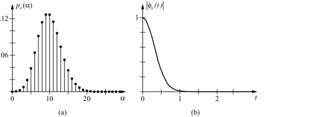
0 10 20
x
p (α) .12
.06
(a)
1
x(t )
t
0 1 2
(b)
φ
α
FIGURE 5.7: (a) PMF and (b) magnitude characteristic function for Poisson distributed RV with parameterλ=10.
Figure 5.7 illustrates the PMF and characteristic function magnitude for a discrete RV with Poisson distribution and parameterλ=10.
It is of interest to note that if x1and x2are independent Poisson RVs with parametersλ1 andλ2, respectively, then
φx1+x2(t)=exp((λ1+λ2)(e
j t−
1)); (5.49)
i.e., x1+x2is also a Poisson with parameterλ1+λ2.
The moments of a Poisson RV are tedious to compute using techniques we have seen so far. Consider the function
ψx(γ)=E(γx) (5.50)
and note that
ψ(k)
x (γ)= E
γx−k
k−1
i=0 (x−i)
,
so that
E
k−1
i=0 (x−i)
=ψ(k)
x (1). (5.51)
If x is Poisson distributed with parameterλ, then
ψx(γ)=eλ(γ−1), (5.52)
so that
ψ(k)
hence,
E
k−1
i=0 (x−i)
=λk. (5.53)
In particular, E(x)=λ, E(x(x−1))=λ2 =E(x2)−λ, so thatσ2
x =λ2+λ−λ2 =λ.
While it is quite easy to calculate the value of the Poisson PMF for a particular number of successes, hand computation of the CDF is quite tedious. Therefore, the Poisson CDF is tabulated in Tables A.4-A.7 of the Appendix for selected values of λranging from 0.1 to 18. From the Poisson CDF table, we note that the value of the Poisson PMF increases as the number of successes k increases from zero to the mean, and then decreases in value as k increases from the mean. Additionally, note that the table is written with a finite number of entries for each value ofλbecause the PMF values are written with six decimal place accuracy, even though an infinite number of Poisson successes are theoretically possible.
Example 5.4.1. On the average, Professor Rensselaer grades 10 problems per day. What is the
probability that on a given day (a) 8 problems are graded, (b) 8–10 problems are graded, and (c) at least 15 problems are graded?
Solution. With x a Poisson random variable, we consult the Poisson CDF table withλ=10, and find
a) px(8)=Fx(8)−Fx(7)=0.3328−0.2202=0.1126,
b) P (8≤x ≤10)= Fx(10)−Fx(7)=0.5830−0.2202=0.3628,
c) P (x ≥15)=1−Fx(14)=1−0.9165=0.0835.
5.4.1 Interarrival Times
In many instances, the length of time between successes, known as an interarrival time, of a Poisson random variable is more important than the actual number of successes. For example, in evaluating the reliability of a medical device, the time to failure is far more significant to the biomedical engineer than the fact that the device failed. Indeed, the subject of reliability theory is so important that entire textbooks are devoted to the topic. Here, however, we will briefly examine the subject of interarrival times from the basis of the Poisson PMF.
Let RV tr denote the length of the time interval from zero to the r th success. Then
p(τ −h <tr ≤τ)= p(r−1, τ −h) p(1,h)
so that
Ftr(τ)−Ftr(τ −h)
h =λp(r −1, τ −h)+ o (h)
h .
Taking the limit as h →0 we find that the PDF for the r th order interarrival time, that is, the time interval from any starting point to the r th success after it, is
ftr(τ)=
λrτr−1e−λτ
(r −1)! u(τ), r =1,2, . . . . (5.54)
This PDF is known as the Erlang PDF. Clearly, with r =1, we have the exponential PDF:
ft(τ)=λe−λτu(τ). (5.55)
The RV t is called the first-order interarrival time.
The Erlang PDF is a special case of the gamma PDF:
fx(α)=
λrαr−1e−λα
(r ) u(α), (5.56)
for any real r >0,λ >0, whereis the gamma function
(r )=
∞
0
αr−1e−αdα. (5.57)
Straightforward integration reveals that(1)=1 and(r +1)=r(r ) so that if r is a positive integer then(r )=(r −1)!—for this reason the gamma function is often called the factorial function. Using the above definition for (r ), it is easily shown that the moment generating function for a gamma-distributed RV is
Mx(η)=
λ
λ−η
r
, for η < λ. (5.58)
The characteristic function is thus
φx(t)=
λ λ− j t
r
. (5.59)
It follows that the mean and variance are
ηx =
r
λ, and σx2=
r
λ2. (5.60)
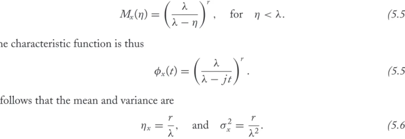
0 20 40
x
f (α) .06
.03
(a)
1
x(t )
t
0 1 2
(b)
φ
α
FIGURE 5.8: (a) PDF and (b) magnitude characteristic function for gamma distributed RV with r =3 and parameterλ=0.2.
Drill Problem 5.4.1. On the average, Professor S. Rensselaer makes five blunders per lecture.
Determine the probability that she makes (a) less than six blunders in the next lecture: (b) exactly five blunders in the next lecture: (c) from three to seven blunders in the next lecture: (d) zero blunders in the next lecture.
Answers: 0.6160, 0.0067, 0.7419, 0.1755.
Drill Problem 5.4.2. A process yields 0.001% defective items. If one million items are produced,
determine the probability that the number of defective items exceeds twelve.
Answer: 0.2084.
Drill Problem 5.4.3. Professor S. Rensselaer designs her examinations so that the probability of at
least one extremely difficult problem is 0.632. Determine the average number of extremely difficult problems on a Rensselaer examination.
Answer: 1.
5.5
UNIVARIATE GAUSSIAN DISTRIBUTION
Definition 5.5.1. A continuous RV z is a standardized Gaussian RV if the PDF is
fz(α)=
1 √
2πe
−1
2α2. (5.61)
The moment generating function for a standardized Gaussian RV can be found as follows:
Mz(λ)=
1 √
2π
∞
−∞
eλα−12α2dα
= √1 2π
∞
−∞
e−12((α−λ)2−λ2)dα.
Making the change of variableβ =α−λwe find
Mz(λ)=e
1 2λ
2
∞
−∞
fz(β)dβ =e
1 2λ
2
, (5.62)
for all realλ. We have made use of the fact that the function fzis a bona fide PDF, as treated
in Problem 42. Using the Taylor series expansion for an exponential,
e12λ2 =
∞
k=0 λ2k 2kk! =
∞
n=0 M(n)
x (0)λn
n! ,
so that all moments of z exist and
E(z2k)= (2k)!
2kk!, k =0,1,2, . . . , (5.63)
and
E(z2k+1)=0, k =0,1,2, . . . . (5.64)
Consequently, a standardized Gaussian RV has zero mean and unit variance. Extending the range of definition of Mz(λ) to include the finite complex plane, we find that the characteristic
function is
φz(t)= Mz( j t)=e−
1
2t2. (5.65)
Letting the RV x =σz+ηwe find that E(x)=ηandσ2
x =σ2. Forσ >0
so that x has the general Gaussian PDF
fx(α)=
1 √
2πσ2exp
− 1
2σ2(α−η) 2
. (5.66)
Similarly, withσ >0 and x = −σz+ηwe find
Fx(α)= P (−σz+η≤α)=1−Fz((η−α)/σ),
so that fx is as above. We will have occasion to use the shorthand notation x∼G(η, σ2) to
denote that the RV has a Gaussian PDF with meanηand varianceσ2. Note that if x ∼G(η, σ2) then (x=σz+η)
φx(t)=ejηte−
1
2σ2t2. (5.67)
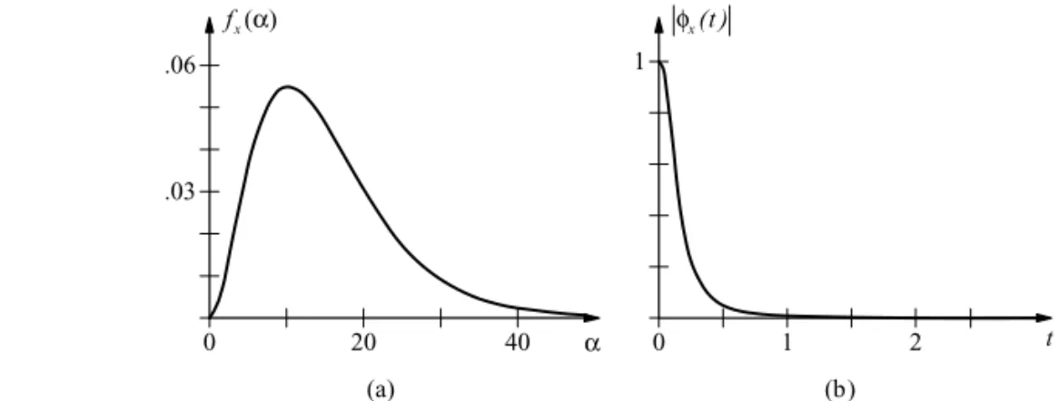
The Gaussian PDF, illustrated withη=75 andσ2=25, as well as withη=75 andσ2=9 in Figure 5.9, is a bell-shaped curve completely determined by its mean and variance. As can be seen, the Gaussian PDF is symmetrical about the vertical axis through the expected value. If, in fact, η=25, identically shaped curves could be drawn, centered now at 25 instead of 75. Additionally, the maximum value of the Gaussian PDF, (2πσ2)−1/2, occurs atα =η. The PDF approaches zero asymptotically asαapproaches±∞. Naturally, the larger the value of the variance, the more spread in the distribution and the smaller the maximum value of the PDF. For any combination of the mean and variance, the Gaussian PDF curve must be symmetrical as previously described, and the area under the curve must equal one.
Unfortunately, a closed form expression does not exist for the Gaussian CDF, which necessitates numerical integration. Rather than attempting to tabulate the general Gaussian CDF, a normalization is performed to obtain a standardized Gaussian RV (with zero mean
α
x
f (α)
.12
65 75 85
.08
.04
and unit variance). If x ∼G(η, σ2), the RV z=(x−η)/σ is a standardized Gaussian RV: z∼G(0,1). This transformation is always applied when using standard tables for computing probabilities for Gaussian RVs. The probability P (α1<x≤α2) can be obtained as
P (α1<x≤α2)= Fx(α2)−Fx(α1), (5.68)
using the fact that
Fx(α)= Fz((α−η)/σ). (5.69)
Note that
Fz(α)=
1 √
2π α
−∞
e−12τ2dτ =1−Q(α), (5.70)
where Q(·) is Marcum’s Q function:
Q(α)= √1 2π
∞
α
e−12τ 2
dτ. (5.71)
Marcum’s Q function is tabulated in Tables A.8 and A.9 for 0≤α <4 using the approximation presented in Section 5.5.1. It is easy to show that
Q(−α)=1−Q(α)=Fz(α). (5.72)
The error and complementary error functions, defined by
erf(α)= 2 π
α
0
e−t2d t (5.73)
and
erfc(α)= 2 π
∞
α
e−t2d t=1−erf(α) (5.74)
are also often used to evaluate the standard normal integral. A simple change of variable reveals that
erfc(α)=2Q(α/√2). (5.75)
Solution. To compute Fz(−1.74), we find
Fz(−1.74)=1−Q(−1.74)=Q(1.74)=0.04093,
using (5.72) and Table A.8.
While the value a Gaussian random variable takes on is any real number between negative infinity and positive infinity, the realistic range of values is much smaller. From Table A.9, we note that 99.73% of the area under the curve is contained between −3.0 and 3.0. From the transformation z=(x−η)/σ, the range of values random variable x takes on is then approximatelyη±3σ. This notion does not imply that random variable x cannot take on a value outside this interval, but the probability of it occurring is really very small (2Q(3)=0.0027).
Example 5.5.2. Suppose x is a Gaussian random variable withη=35 andσ =10. Sketch the PDF and then find P (37≤x≤51). Indicate this probability on the sketch.
Solution. The PDF is essentially zero outside the interval [η−3σ, η+3σ]=[5,65]. The sketch of this PDF is shown in Figure 5.10 along with the indicated probability. With
z= x−35 10
we have
P (37≤x ≤51)= P (0.2≤z≤1.6)= Fz(1.6)−Fz(0.2).
Hence P (37≤ x≤51)= Q(0.2)−Q(1.6)=0.36594 from Table A.9.
x
f (α)
.03
30 60
.02 .01 .04
0 α
Example 5.5.3. A machine makes capacitors with a mean value of 25μF and a standard deviation of 6μF. Assuming that capacitance follows a Gaussian distribution, find the probability that the value of capacitance exceeds 31μF if capacitance is measured to the nearestμF.
Solution. Let the RV x denote the value of a capacitor. Since we are measuring to the nearest
μF, the probability that the measured value exceeds 31μF is
P (31.5≤ x)= P (1.083≤z)= Q(1.083)=0.13941,
where z=(x−25)/6∼G(0,1). This result is determined by linear interpolation of the CDF
between equal 1.08 and 1.09.
5.5.1 Marcum’s Q Function Marcum’s Q function, defined by
Q(γ)= √1 2π
∞
γ
e−12α2dα (5.76)
has been extensively studied. If the RV z∼G(0,1) then
Q(γ)=1−Fz(γ); (5.77)
i.e., Q(γ) is the complement of the standard Gaussian CDF. Note that Q(0)=0.5, Q(∞)=0, and that Fz(−γ)=Q(γ). A very accurate approximation to Q(γ) is presented in [1, p. 932]:
Q(γ)≈e−12γ 2
h(t), γ >0, (5.78)
where
t = 1
1+0.2316419γ, (5.79)
and
h(t)= √1
2πt(a1+t(a2+t(a3+t(a4+a5t)))). (5.80) The constants are
i ai
A very useful bound for Q(α) is [1, p. 298]
2 π
e−12α 2
α+√α2+4 <Q(α)≤
2 π
e−12α 2
α+√α2+0.5π. (5.81) The ratio of the upper bound to the lower bound is 0.946 whenα=3 and 0.967 whenα =4. The bound improves asαincreases.
Sometimes, it is desired to find the value ofγ for which Q(γ)=q . Helstrom [14] offers an iterative procedure which begins with an initial guessγ0>0. Then compute
ti =
1 1+0.2316419γi
(5.82)
and
γi+1=
2 ln
h(ti)
q
1/2
, i =0,1, . . . . (5.83)
The procedure is terminated whenγi+1 ≈γi to the desired degree of accuracy.
Drill Problem 5.5.1. Students attend Fargo Polytechnic Institute for an average of four years with a
standard deviation of one-half year. Let the random variable x denote the length of attendance and as-sume that x is Gaussian. Determine: (a) P (1<x <3),(b)P (x>4),(c )P (x=4),(d )Fx(4.721).
Answers: 0.5, 0, 0.02275, 0.92535.
Drill Problem 5.5.2. The quality point averages of 2500 freshmen at Fargo Polytechnic Institute
follow a Gaussian distribution with a mean of 2.5 and a standard deviation of 0.7. Suppose grade point averages are computed to the nearest tenth. Determine the number of freshmen you would expect to score: (a) from 2.6 to 3.0, (b) less than 2.5, (c) between 3.0 and 3.5, (d) greater than 3.5.
Answers: 167, 322, 639, 1179.
Drill Problem 5.5.3. Professor Rensselaer loves the game of golf. She has determined that the distance
the ball travels on her first shot follows a Gaussian distribution with a mean of 150 and a standard deviation of 17. Determine the value of d so that the range, 150±d , covers 95% of the shots.
Answer: 33.32.
5.6
BIVARIATE GAUSSIAN RANDOM VARIABLES
Numerous applications of this joint PDF are found throughout the field of biomedical engi-neering and, like the univariate case, the joint Gaussian PDF is considered the most important joint distribution for biomedical engineers.
Definition 5.6.1. The bivariate RV z=(x,y) is a bivariate Gaussian RV if every linear combi-nation of x and y has a univariate Gaussian distribution. In this case we also say that the RVs x and y are jointly distributed Gaussian RVs.
Let the RV w=a x+b y, and let x and y be jointly distributed Gaussian RVs. Then w is a univariate Gaussian RV for all real constants a and b. In particular, x ∼G(ηx, σx2) and
y ∼G(ηy, σy2); i.e., the marginal PDFs for a joint Gaussian PDF are univariate Gaussian. The
above definition of a bivariate Gaussian RV is sufficient for determining the bivariate PDF, which we now proceed to do.
The following development is significantly simplified by considering the standardized versions of x and y. Also, we assume that|ρx,y|<1,σx =0, andσy =0. Let
z1= x−ηx
σx
and z2= y−ηy
σy
, (5.84)
so that z1∼G(0,1) and z2∼G(0,1). Below, we first find the joint characteristic function for the standardized RVs z1and z2, then the conditional PDF fz2|z1 and the joint PDF fz1,z2. Next, the results for z1and z2are applied to obtain corresponding quantitiesφx,y, fy|x and fx,y.
Finally, the special casesρx,y = ±1,σx =0, andσy =0 are discussed.
Since z1and z2are jointly Gaussian, the RV t1z1+t2z2is univariate Gaussian:
t1z1+t2z2∼G
0,t12+2t1t2ρ+t22.
Completing the square,
t12+2t1t2ρ+t22=(t1+ρt2)2+(1−ρ2)t22,
so that
φz1,z2(t1,t2)=E(e
j t1z1+j t2z2)=e−12(1−ρ2)t22e−12(t1+ρt2)2. (5.85)
From (6) we have
fz1,z2(α, β)= 1 2π
∞
−∞
where
I (α,t2)= 1 2π
∞
−∞
φz1,z2(t1,t2)e
−jαt1d t1.
Substituting (5.85) and lettingτ =t1+t2ρ, we obtain
I (α,t2)=e−12(1−ρ2)t 2 2 1
2π
∞
−∞
e−12τ2e−jα(τ−ρt2)dτ,
or
I (α,t2)=φ(t2) fz1(α),
where
φ(t2)=ejαρt2e−12(1−ρ2)t22.
Substituting into (5.86) we find
fz1,z2(α, β)= fz1(α) 1 2π
∞
−∞
φ(t2)e−jβt2d t 2
and recognize thatφis the characteristic function for a Gaussian RV with meanαρand variance 1−ρ2. Thus
fz1,z2(α, β) fz1(α)
= fz2|z1(β|α)=
1
2π(1−ρ2)exp
−(β−ρα)2 2(1−ρ2)
, (5.87)
so that
E(z2|z1)=ρz1 (5.88)
and
σ2
z2|z1 =1−ρ
2. (5.89)
After some algebra, we find
fz1,z2(α, β)=
1
2π(1−ρ2)1/2exp
−α2−2ραβ+β2 2(1−ρ2)
. (5.90)
We now turn our attention to using the above results for z1and z2to obtain similar results for x and y. From (5.84) we find that
so that the joint characteristic function for x and y is
φx,y(t1,t2)= E(ej t1x+j t2y)=E(ej t1σxz1+j t2σyz2)ej t1ηx+j t2ηy.
Consequently, the joint characteristic function for x and y can be found from the joint charac-teristic function of z1and z2as
φx,y(t1,t2)=φz1,z2(σxt1, σyt2)e
jηxt1ejηyt2. (5.91)
Using (4.66), the joint characteristic functionφx,ycan be transformed to obtain the joint PDF
fx,y(α, β) as
fx,y(α, β)=
1 (2π)2
∞ −∞ ∞ −∞
φz1,z2(σxt1, σyt2)e
−j (α−ηx)t1e−j (β−ηy)t2d t
1d t2. (5.92)
Making the change of variablesτ1=σxt1,τ2=σyt2, we obtain
fx,y(α, β)=
1 σxσy
fz1,z2
α−η
x
σx ,
β−ηy
σy
. (5.93)
Since
fx,y(α, β)= fy|x(β|α) fx(α)
and
fx(α)=
1 σx
fz1
α−η
x
σx
,
we may apply (5.93) to obtain
fy|x(β|α)=
1 σy
fz2|z1
β−η
y
σy
α−ηx
σx
. (5.94)
Substituting (5.90) and (5.87) into (5.93) and (5.94) we find
fx,y(α, β)=
exp
− 1 2(1−ρ2)
(α−ηx)2
σ2
x −
2ρ(α−ηx)(β−ηy) σxσy +
(β−ηy)2 σ2
y
2πσxσy(1−ρ2)1/2
(5.95)
and
fy|x(β|α)=
exp
−
β−ηy−ρσyα−σηx x
2
2(1−ρ2)σ2 y
2πσ2
y(1−ρ2)
It follows that
E(y|x)=ηy+ρσy
x−ηx
σx
(5.97)
and
σ2
y|x =σy2(1−ρ2). (5.98)
By interchanging x with y andαwithβ,
fx|y(α|β)=
exp ⎛
⎝−
α−ηx−ρσxβ−η y σy
2
2(1−ρ2)σ2 y
⎞ ⎠
2πσ2
x(1−ρ2)
, (5.99)
E(x|y)=ηx+ρσx
y−ηy
σy ,
(5.100)
and
σ2
x|y =σx2(1−ρ2). (5.101)
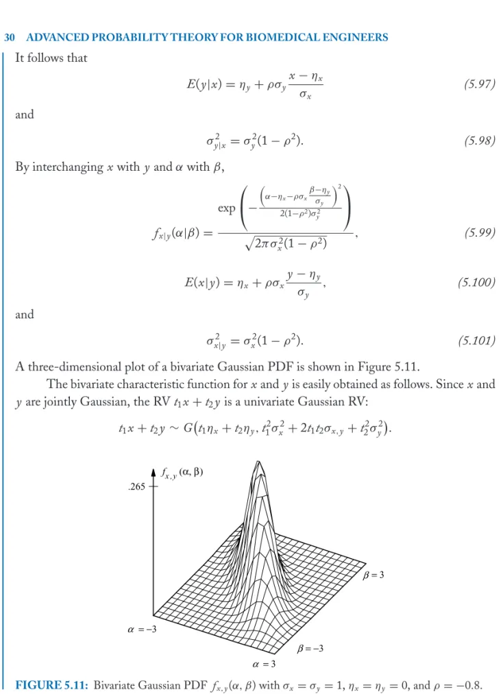
A three-dimensional plot of a bivariate Gaussian PDF is shown in Figure 5.11.
The bivariate characteristic function for x and y is easily obtained as follows. Since x and y are jointly Gaussian, the RV t1x+t2y is a univariate Gaussian RV:
t1x+t2y ∼G
t1ηx+t2ηy,t12σx2+2t1t2σx,y+t22σy2
.
x ,y f (α, β ) .265
α = −3
α =3
β = −3
β =3
Consequently, the joint characteristic function for x and y is
φx,y(t1,t2)=e−
1
2(t12σx2+2t1t2σx,y+t2
2σ2y)ej t1ηx+j t2ηy, (5.102)
which is valid for allσx,y,σx andσy.
We now consider some special cases of the bivariate Gaussian PDF. Ifρ=0 then (from (5.95))
fx,y(α, β)= fx(α) fy(β); (5.103)
i.e., RVs x and y are independent.
Asρ→ ±1, from (5.97) and (5.98) we find
E(y|x)→ηy±σy
x−ηx
σx
andσy2|x →0. Hence,
y →ηy±σy
x−ηx
σx
in probability1. We conclude that
fx,y(α, β)= fx(α)δ
β−ηy±σyα−ηx
σx
(5.104)
forρ= ±1. Interchanging the roles of x and y we find that the joint PDF for x and y may also be written as
fx,y(α, β)= fy(β)δ
α−ηx ±σx
β−ηy
σy
(5.105)
whenρ= ±1. These results can also be obtained “directly” from the joint characteristic function for x and y.
A very special property of jointly Gaussian RVs is presented in the following theorem.
Theorem 5.6.1. The jointly Gaussian RVs x and y are independent iffρx,y =0.
Proof. We showed previously that if x and y are independent, thenρx,y =0.
Suppose thatρ=ρx,y =0. Then fy|x(β|α)= fy(β).
Example 5.6.1. Let x and y be jointly Gaussian with zero means,σ2
x =σy2=1, andρ= ±1.
Find constants a and b such that v=a x+b y ∼G(0,1) and such that v and x are independent.
Solution. We have E(v)=0. We require
σ2
v =a
2+
b2+2abρ2x,y =1
and
E(vx)=a +bρx,y =0.
Hence a = −bρx,yand b2=1/(1−ρx2,y), so that
v= y−ρx,yx 1−ρ2
x,y
is independent of x andσv2=1.
5.6.1 Constant Contours
Returning to the normalized jointly Gaussian RVs z1and z2, we now investigate the shape of the joint PDF fz1,z2(α, β) by finding the locus of points where the PDF is constant. We assume that|ρ|<1. By inspection of (5.90), we find that fz1,z2(α, β) is constant forαandβsatisfying
α2−2ραβ+β2=c2, (5.106)
where c is a positive constant.
Ifρ =0 the contours where the joint PDF is constant is a circle of radius c centered at the origin.
Along the lineβ =qαwe find that
α2(1−2ρq +q2)=c2 (5.107)
so that the constant contours are parameterized by
α = ±c
1−2ρq +q2, (5.108)
and
β = ±c q
1−2ρq +q2. (5.109)
The square of the distance from a point (α, β) on the contour to the origin is given by
d2(q )=α2+β2= c
2(1+q2)
Differentiating, we find that d2(q ) attains its extremal values at q = ±1. Thus, the lineβ =α intersects the constant contour at
±β =α= ±c
2(1−ρ). (5.111)
Similarly, the lineβ = −α, intersects the constant contour at
±β = −α = ±c
2(1−ρ). (5.112)
Consider the rotated coordinatesα =(α+β)/√2 andβ =(β−α)/√2, so that
α +β
√
2 =β (5.113)
and
α −β
√
2 =α. (5.114)
The rotated coordinate system is a rotation byπ/4 counterclockwise. Thus
α2−2ραβ+β2=c2 (5.115)
is transformed into
α2 1+ρ +
β2 1−ρ =
c2
1−ρ2. (5.116)
The above equation represents an ellipse with major axis length 2c/√1− |ρ|and minor axis length 2c/√1+ |ρ|. In theα−β plane, the major and minor axes of the ellipse are along the linesβ = ±α.
From (5.93), the constant contours for fx,y(α, β) are solutions to
α−η x σx 2 −2ρ α−η x σx
β−ηy
σy + β−η y σy 2
=c2. (5.117)
Using the transformation
α = √1
2
α−η
x
σx +
β−ηy
σy
, β = √1
2
β−η
y
σy −
α−ηx
σx
(5.118)
transforms the constant contour to (5.116). Withα =0 we find that one axis is along α−ηx
σx = −
β−ηy
with endpoints at
α = ±cσx
√
2√1+ρ +ηx, β =
±cσy
√
2√1+ρ +ηy;
the length of this axis in theα−β plane is
√ 2c
σ2
x +σy2
1+ρ .
Withβ =0 we find that the other axis is along
α−ηx
σx =
β−ηy
σy
with endpoints at
α = ±cσx
√
2√1−ρ +ηx, β =
±cσy
√
2√1−ρ +ηy;
the length of this axis in theα−β plane is
√ 2c
σ2
x +σy2
1−ρ .
Points on this ellipse in theα−β plane satisfy (5.117); the value of the joint PDF fx,y on this
curve is
1 2πσxσy
1−ρ2exp
− c2 2(1−ρ2)
. (5.119)
A further transformation
α = √α
1+ρ, β
= √β
1−ρ
transforms the ellipse in theα −β plane to a circle in theα −β plane:
α 2+β 2= c2 1−ρ2.
![Figure 5.2 illustrates the PDF and the magnitude of the characteristic function for a continuous RV uniformly distributed on [0, 1]](https://thumb-us.123doks.com/thumbv2/123dok_es/5679850.133959/11.918.139.809.447.735/figure-illustrates-magnitude-characteristic-function-continuous-uniformly-distributed.webp)