Essays on Inflation, Real Stock Prices, and
Extreme Macroeconomic Events
Diego Pereira-Garmendia
TESI DOCTORAL UPF / 2011
DIRECTOR DE LA TESI
Dipòsit Legal: ISBN:
A
CKNOWLEDGMENTS
“Now this is not the end. It is not even the beginning of the end. But it is, perhaps, the end of the
beginning.”
(Sir Winston Churchill, Speech in November 1942)
Foremost, I would like to express my deepest gratitude to my advisor Joachim Voth. His patience, suggestions, comments, and criticisms have been truly invaluable.
Many thanks to Fernando Broner, Francisco Peñaranda, Jaume Ventura, Angel León, Gonzalo Rubio, and Vicente Ortún for their suggestions and encouragement. The acknowledgement is extensive to all the participants of the UPF International and Finance Lunch for comments and suggestions.
Durant aquest temps, he tingut la sort de trobar-me amb uns com-panys que han esdevingut alhora amics. It is a rewarding long list: Federico Todeschini, Andrea Tesei, Peter Hoffmann, Pablo Fleiss, Francesco Caprioli, Pablo Brassiolo, Onuralp Soylemez, Takuji Okubo, Zeynep Gurguc, Basak Gunes, Filippo Ferroni, Filippo Brutti, Nico Voigtländer, Stan Veuger, Deny Bobula, Clarisse Coelho, Torsten Santavirta, Juan Martin Moreno, Sumit Sharma, Javier Valbuena, Ain-hoa Aparicio, Paulo Abecasis, Goncalo Pina, Maria Paula Gerardino, Burak Ok, Shikeb Farooqui, Jacopo Ponticelli, Juan Manuel Puerta, and Ignacio Fernandez.
To all the GPEFM Devils, for which I served both as player and ‘mister’, and even with that handicap we came to be champions.
Many thanks to Marta Araque, Laura Agustí, and Mariona Novoa for making everything easier during these years.
To Dolores and Ezequiel, and to Father Javier.
& Anne & Lucca (alias ahijado) & Franco; Martin & Andrea & Eu-genia, and Andrés & Janet & Antonella. I also want to thank CERES and Dr. Ernesto Talvi for his guidance and encouragement.
Finally and most importantly, to my parents Sara and Pedro for their continuos support and encouragement. For them and because of them is this work. To Mario and Ignacio, who often have behaved like my older brothers. And finally, my girlfriend Ester, who has accompanied me on this journey.
Barcelona, June 2011.
A
BSTRACT
This thesis examines the negative correlation between inflation and real stock prices. First, using an Emerging Market data sample, I find robust evidence for inflation imposing real costs on the economy, in particular by decreasing firms’ real earnings as originally claimed by Milton Friedman. The results limit the need for behavioral explanations. Second, I suggest that increasing inflation led to lower real stock prices as the probability of experiencing a stagflation episode increases (rare-event premium). Third, I test whether macroeconomic data provide evidence for a positive correla-tion between inflacorrela-tion and uncertainty, and between inflacorrela-tion and the price of risk (i.e. relative risk aversion), as suggested in the literature. Fourth, I introduce a historical case, Germany between 1870 and 1935, and show that it is the rare-event premium, not money illusion, what drives the negative relation between inflation and stock prices. The fifth chapter is a separate work on emerging markets financial contagion.
R
ESUMEN
F
OREWORD
This dissertation includes five chapters, of which the first four chap-ters are dedicated to investigate the relationship between inflation and real stock prices. The last chapter is a separate work on Emerging Market financial contagion.
In the last 30 years the relation between inflation and real stock prices has been widely discussed in the literature. If stocks are a claim on real capital, the covariance between real stock prices and inflation should be zero. However, the empirical findings show a robust nega-tive correlation between inflation (realized, expected and unexpected) and real stock prices. This is known as the ‘stock price-inflation puz-zle’.
A number of models have been developed to explain the ‘stock price-inflation puzzle’. However, the lack of robust empirical evi-dence for the different channels suggested in the literature has led the authors to support behavioural factors. The behavioural approach mostly relies on money illusion: investors confuse nominal and real discount rates. Thus, given future real cash flows, higher inflation leads to higher discount rates (nominal interest rates), and therefore to lower stock prices (cf. Modigliani and Cohn, 1979; and Campbell and Vuolteenaho, 2004).
In Chapters 1 to 4, I introduce empirical evidence that questions the need to build on money illusion and related behavioural approaches. Moreover, I discuss how the negative correlation between inflation and real stock prices could be explained by agents discounting future rare macroecomic events (rare-event premium). I also test whether the macroeconomic data back some of the common assumptions that the literature has recently made on the inflation and risk relationship. Finally, I show that the rare-event premium hypothesis is more robust than the behavioural hypothesis.
claimed by Milton Friedman (1971, 1977). The results limit the need for behavioural explanations.
In Chapter 2, I work on an explanation for the positive correlation between inflation and risk. In this framework, realized inflation is used as a proxy for the probability of a rare event, namely high infla-tion accompanied by stalling or negative economic growth (stagfla-tion). When agents observe increasing inflation rates, they perceive an increase in the probability of experiencing a stagflation episode in the future. Consequently, agents demand a higher premium. The model predicts a positive relation between the correlation of inflation and real stock prices, and both uncertainty and risk aversion. I test the model implications for the US and Germany, and find empirical support for the model predictions.
The third chapter is dedicated to test whether macroeconomic data provide evidence for a positive correlation between inflation and uncertainty, and between inflation and the price of risk (i.e. rela-tive risk aversion). It has been suggested that the ‘real stock prices-inflation puzzle’ could be explained by an unconditional positive re-lation between infre-lation and risk (cf. Brandt and Wang, 2003; and Bekaert and Engstrom, 2010). The results show that there is a strong relation between inflation and uncertainty, but only for inflation lev-els above 10 percent (annualized rates). Also, the positive relation between inflation and risk aversion is not robust for inflation regimes below 10 percent, or above 50 percent. However, I find evidence for a monotonic relation between inflation and stagflation risk premium (rare-event premium) discussed in Chapter 2.
Chapter 4 introduces a historical case, German economy between 1870 and 1935, to show that it is the rare-event premium, not money illusion, what drives the negative relation between inflation and stock prices. While testing for money illusion is an elusive quest, I dis-cuss two cases that help to differentiate the rare-event premium from money illusion. First, the rare-event premium is state-dependent while money illusion is not. Second, inflation must belong to the invest-ment set (understood as the set of all dimensions relevant to an in-vestment decision) for the rare-event premium explanation to make sense. However, this is not true in the case of money illusion. Even if price changes are not giving any information on future inflation rates, agents will continue to use nominal discount rates instead of real dis-count rates. Using data on the Gold Standard period, as well as the
inflation period (1921-23), I find evidence supporting the rare-event premium explanation.
C
ONTENTS
Abstract . . . vii
Foreword . . . ix
1 Inflation, Real Stock Prices and Earnings: Friedman Was Right 7 1.1 Introduction . . . 7
1.2 Data Description . . . 11
1.3 Method and Results . . . 14
1.3.1 Real Stock Prices and Inflation . . . 15
1.3.1.1 Real Stock Price, Inflation Level and Inflation Volatility . . . 18
1.3.1.2 Asymmetric Crisis Effects . . . 19
1.3.2 Inflation and Real Earnings . . . 21
1.3.2.1 Non-Linearities . . . 24
1.3.2.2 Quantifying the impact of decreas-ing real earndecreas-ings growth rates on real stock price variations . . . 25
1.4 Sector Analysis . . . 26
1.4.1 Sector-Portfolio Specification . . . 28
1.5 Discussion and Conclusions . . . 31
2 Explaining the Stock Price-Inflation Puzzle: Inflation as a Signal for a Stagflation Event 53 2.1 Introduction . . . 53
2.2 Inflation as a Signal for the Bad State and Stock Prices 58 2.2.1 Setup . . . 59
2.3 Inflation, Stagflation Beliefs and Stock Prices . . . . 60
2.3.1 Time-Independent Probability of Stagflation . 61 2.3.2 Time-Dependent Probability of Rare Events . 63 2.3.2.1 Bayesian Belief Updating . . . 65
2.4 Empirical Implementation . . . 67
2.4.1 Markov Switching Regime Estimation . . . . 67
2.4.4 Other Inflation Measures . . . 74
2.4.5 The German Case . . . 75
2.5 Testing Other Nominal Signals . . . 76
2.5.1 Investment Opportunity Set . . . 77
2.5.2 Markov Switching Regime Estimation . . . . 78
2.6 2008-2010: Crisis, Recession and Stagflation Proba-bility . . . 79
2.7 Conclusions . . . 81
3 Inflation, Uncertainty and Price of Risk: Let Data Speak for Itself 105 3.1 Introduction . . . 105
3.2 Data . . . 109
3.2.1 Inflation Regimes . . . 110
3.2.2 Transition Probability Matrices . . . 110
3.3 Inflation and Uncertainty . . . 112
3.3.1 Regime-Conditional Real Consumption Growth Rates Distribution . . . 112
3.3.2 Regime-Conditional Return Distribution . . . 114
3.4 Inflation and Price of Risk . . . 116
3.4.1 Simulation of Regime-Conditional Expected Returns . . . 116
3.4.2 Regime-Implicit Relative Risk Aversion (RRA) Coefficient . . . 120
3.4.2.1 Power Utility . . . 120
3.4.2.2 Epstein-Zin-Weil Preferences . . . 124
3.5 Stagflation Risk . . . 126
3.5.1 Stagflations as Macro-Disasters . . . 126
3.5.2 Regime-Conditional Probability of a Stock Price Collapse . . . 128
3.6 Conclusions . . . 131
4 Inflation and Risk Aversion: Rare-Event Premium or Money Illusion? 151 4.1 Introduction . . . 151
4.2 Rare-Event Premium . . . 156
4.3 Empirical Implementation . . . 159
4.3.1 Stock Premium Under Money Illusion Hy-pothesis . . . 159
4.3.2 Stock Premium under Rare-Event Hypothesis 161 4.3.3 Money Illusion or Rare Event Premium? . . 162
4.4 Germany Post-WWI: Reparations, Inflation, Recov-ery and Depression . . . 163
4.4.1 The Road to Hyperinflation . . . 163
4.4.2 The Inflation Period: June 1922 - November 1923 . . . 167
4.4.3 Post-Inflation: Economic Recovery . . . 169
4.5 Estimation and Results . . . 171
4.5.1 Data . . . 171
4.5.2 VAR Estimation . . . 171
4.5.3 Expected Inflation: VAR Forecast vs Forward Exchange Market . . . 172
4.5.4 Stock Premium . . . 173
4.5.5 Expected Dividend Growth Rate . . . 175
4.5.6 Stock Premium Decomposition . . . 178
4.6 Is It Rare Event Premium or Money Illusion? . . . . 180
4.6.1 State Dependency . . . 181
4.6.2 Inflation not Included in Investment Set . . . 182
4.7 Robustness . . . 184
4.7.1 Standard VAR Estimation Robustness . . . . 185
4.7.2 Error-Space and Rare-Event Premium . . . . 185
4.7.3 Time-Varying-Parameter VAR Estimation . . 187
4.8 Discussion and Conclusions . . . 189
5 US Cold, Worldwide Pneumonia: American Fama-French Factors Drive Contagion 213 5.1 Introduction . . . 213
5.2 EM Spreads, American Fama-French Factors and Con-tagion . . . 219
5.2.2 EM Spreads and American Fama-French Fac-tors: Long and Short-Run Relationship . . . 222 5.3 Principal Component Analysis . . . 227
5.3.1 Principal Component Analysis for EM and USC spreads . . . 227 5.3.1.1 Sample I: US Corporate Spreads and
EMBI+ . . . 228 5.3.1.2 Sample II: 13 Emerging Countries
EMBI+ spread . . . 228 5.3.2 Global Risk Aversion and American
Fama-French Factors . . . 229 5.3.2.1 Global Risk Aversion and
Ameri-can Fama-French Factors: US Cor-porate Bonds . . . 229 5.3.2.2 Global Investment Appetite and
Amer-ican Fama-French Factors: Emerg-ing Market Sample . . . 230 5.4 American Fama-French Factors as proxy for Factor
Innovations . . . 232 5.4.1 Factor Innovation Estimation . . . 233 5.4.2 EM Spreads Using Factor Innovations . . . . 234 5.5 EM Stock Markets and American Fama-French Factors235 5.6 Formal Asset Pricing Model Tests . . . 236 5.6.1 Formal Asset Pricing Model Tests: Evidence 236 5.7 Conclusions . . . 238
References 259
A Appendices 273
1 I
NFLATION
, R
EAL
S
TOCK
P
RICES AND
E
ARN
-INGS
: F
RIEDMAN
W
AS
R
IGHT
1.1 I
NTRODUCTION
When inflation increases, stocks fall. Many authors have tried to explain this fact by the performance of real variables. To date, there are no studies showing that real earnings suffer significantly during inflation episodes1. I suggest that the lack of empirical
ev-idence might result from the limiting characteristics of the data on developed countries. In this paper I test for real channels by using data on Emerging Markets. These have the advantage of substantial variation of inflation both across time and countries. The results give support to the idea of inflation imposing real costs on the economy, in particular by decreasing firms’ real earnings as originally claimed by Friedman (1971, 1977). At the same time, the results limit the need for behavioral explanations, e.g. money illusion, as initially suggested by Modigliani and Cohn (1979)2.
In this paper, I test for the existence of three real channels in the case of Emerging Markets (henceforth abbreviated as EMs). First, the direct impact of realized inflation on future real earnings growth rates is tested, controlling for the business cycle and also for non-linearities. Second, the relation between inflation and risk is exam-ined in an indirect way. That is, I show that the correlation between
1Empirical research consistently finds a negative relation between inflation and
real stock prices (i.e. earning yield or dividend yield), e.g. Campbell and Shiller (1988a); Barr and Campbell (1996); Pennacchi (1991); Campbell and Ammer (1993); Amihud (1996) ; Campbell and Shiller (1996); Duarte (2010). Related to this, a number of papers study the negative correlation between bond and stock yields, i.e. Thomas and Zhang (2008); Asness (2002); Bekaert and Engstrom (2010a); Zhang and Thomas (2008); and Durre and Giot (2007).
2Main papers supporting money illusion are Modigliani and Cohn (1979);
stock prices and inflation is significantly higher in recessions (high risk aversion and uncertainty) than in expansions (low risk aversion and uncertainty), while the impact of inflation on real earnings does not show significant variations in recessions when compared to ex-pansion periods. Third, I test for inflation decreasing the real value of nominal liabilities, therefore increasing real stock prices. Note that this last real channel would imply a positive correlation between in-flation and real stock prices, conditional on the firm’s leverage.
Panel estimations are performed instead of the time-series studies present in the literature. This allows me to exploit the rich variation in country, time, and sector, present in the EM sample. The empiri-cal strategy also aims to capture short-term variations, since even the studies disputing the long-run relation between inflation and stock prices (or bond and stock yields) find support for a short-term rela-tion (e.g. Durre and Giot 2007). Therefore, the data frequency for the estimations is monthly3. I perform three different sets of estimations, where the panel unit of analysis is the firm, market and sector, respec-tively. The point is to avoid potential aggregation biases that might otherwise drive the results. In the first specification, the panel unit is each firm in the sample. In this case, the real stock price for each firm is the earning price ratio. In the second specification, the panel unit is the market-portfolio. For that, capital-weighted earnings price ra-tios are used as real stock prices. In the third specification, the panel unit is the sector-portfolio. In this last case, capital-weighted sector earnings price ratios are used as real stock prices. The estimation is adapted to the panel unit: standard and long panel estimations are implemented when working with stocks and portfolios as the panel unit, respectively. The results are robust to the use of different panel units4.
3It is worth to note that the results remain unaltered when working with
quar-terly data.
4Concerns on using monthly frequency for earnings are addressed by using
The literature identifies two real channels under which inflation negatively influences real stock prices. First, inflation decreases fu-ture real earnings growth rates as early papers by Friedman (1971, 1977), and Fama (1981) suggest. For example, inflation hampers in-tertemporal capital allocation (e.g. Aruoba et al. 2009; Chiarella et al. 2007; Brennan and Xia 2002), or acts as a distortionary tax (e.g. Cooley and Hansen 1989; Chari et al. 1996). If these frictions are present, inflation induces a decrease in future real earnings, driving the stock price downward. However, there is as yet no empirical sup-port for a negative correlation between inflation and future real earn-ings. Moreover, some studies point out that the correlation between inflation and real earnings (dividends) is perhaps even positive (e.g. for the US: Asness, 2003; Feinman, 2005; Campbell and Vuoltena-hoo, 2002; and Spyrou, 2004 for emerging countries).
The second real channel relates inflation to risk: inflation corre-lates positively with risk aversion as in Brandt and Wang (2003); or inflation correlates positively with both risk aversion and uncertainty as in Bekaert and Engstrom (2010a)5. As risk increases, investors demand higher expected returns, driving real stock prices downward. Bekaert and Engstrom (2010a) find that the covariance of inflation and risk can explain almost half of the covariance between inflation and real stock prices. However, in the same paper, the authors can-not find a significant covariance between inflation and real earnings growth rates.
The third real channel suggested in the literature is the leverage channel. Under imperfect capital markets, real stock prices may also correlate positively with inflation. Ritter and Warr (2002) suggest
quarterly data. Also, I use year on year as well as quarter on quarter variations when working with earning growth rates.
5Bekaert and Engstrom (2010a) show that inflation is positively related both
that inflation can affect equity value by decreasing the real value of nominal liabilities. For a given expected real cash flow (i.e. firm’s value), inflation decreases real debt, increasing the equity value. The authors do not find evidence of the leverage channel for the US stock market, and refer to this as a valuation error (i.e. debt capital gain error). Note that when the leverage effect is incorporated, the corre-lation between real stock prices and infcorre-lation may even be positive. This happens if the variation in the real stock price owing to inflation eroding the real value of debt is higher than the variation generated by lower real earnings growth rates and higher risk aversion6.
The closest empirical study to the present one is that by Spyrou (2004), since this is the only paper that tests the relation between in-flation and stock returns in EMs. The author studies the relation in a time series framework, the sample including nine EMs for the period 1989-2000. One key point is that the author works only with nomi-nal returns. His results show that in four countries there is a negative relation between inflation and nominal returns. However, he concen-trates on the cases in which inflation correlates positively with nomi-nal returns, and argues that in those cases there is a positive relation between inflation (CPI) and industrial production. The main problem with this approach is that the author is not controlling for real ac-tivity when estimating the covariance between inflation and nominal returns. The estimations then suffer from a strong misspecification, as discussed by Fama (1986).
This paper is structured in the following way. Section 2 describes the data sample. Section 3 introduces the empirical strategy and present the results regarding the correlation between inflation and stock prices, and the presence of real channels. Section 4
comple-6The leverage channel may help us to understand what drives up stock prices
(conditional on expected future dividend growth rate and discount rates) during hyperinflation or very-high-inflation periods (see Chapter 4 and Pereira-Garmendia 2008).
ments the previous analyses by providing new insights at a sector level. Section 5 includes the discussion and concluding remarks.
1.2 D
ATA
D
ESCRIPTION
The data sample spans the period January 1986 to December 2007, on a monthly frequency, for 15 EMs. Earnings price ratios -earning yields- are used as (the inverse of) real stock prices. Trailing earn-ing yields are used, that is, the last 12-month accumulated earnearn-ings over the stock price. The data is from the Emerging Market Database (EMDB). The reason for working with earnings price ratios instead of price-earnings is that the price-earning relation is discontinuous when earnings are close to zero. When creating portfolios, I aggre-gate firm earning yields weighting by the firms’ capital. Both sector and country portfolios are created. Capitalization data comes also from EMDB.
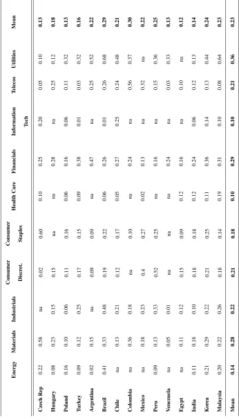
Different aggregation levels for sector data are available. There are 60 sectors in the sample at the lowest level of sector aggregation. These sectors are, at a time, aggregated in a 22-sector ranking, and finally, the highest aggregation level includes ten sectors: Consumer Discretionary, Consumer Staples, Materials, Industrials, Financials, Energy, Utilities, Information Technology, Telecommunication Ser-vices and Health Care.
For leverage, the market debt over capital ratio is used. The data is from Bloomberg, at a firm level, for the years 2006 and 20077.
Since leverage data is only available for 2006 and 2007, I construct sector leverage at lowest level of sector aggregation available (60 sec-tors). In order to construct the series spanning the period 1986-2007,
7While some papers use the Rajan and Zingales (1998) external financial
I weight each firm leverage ratio using capitalization as weights, thus creating variation in time for the sector-leverage series. A key is-sue immediately arises. While it would be optimal to have the actual leverage data for the sample period, due to data limitations, only two years of leverage data is available. In order to create variation in time for 21 years, the assumption placed is that the leverage ordering be-tween sectors does not vary in time. For example, if leverage of Ma-terials is higher than Industrials in 2006-07, then this remains true for the whole period 1986-2007. In Table 1.2 the leverage at highest sec-tor aggregation (10-secsec-tor aggregation) is presented for the countries in the final sample. Note that, sorting per sector, Utilities is the sector with highest leverage, followed by Financials, while the sectors with lowest leverage are Information Technologies and Heath Care.
Inflation data at a monthly frequency is from IMF IFS. The CPI indices are seasonally adjusted, as to avoid noise in the monthly in-flation rates. Figure 1.1 shows the time series for the first, second and third inflation quartile on the left axis, and the fourth quartile on the right axis. Inflation in EMs follows a similar pattern to devel-oped markets. During the 80s, monthly inflation was high and volatile (Great Inflation). After mid-90s, inflation decreased considerably and has remained low and stable since then. Nonetheless, the variation present in EMs -both cross-country and in time- is very high. During the sample period, some of the countries included in the sample expe-rienced long periods of high inflation (higher than 50 percent annual inflation); hyper-inflations (higher than 50 percent monthly inflation); and also long periods of inflation below five percent (in particular the period 2001-2007). It is worth to emphasize that, although in eight percent of the sample the monthly inflation is negative (deflation), only Argentina shows a sequence of consecutive deflationary months from 1999 to 2002 (22 of 36 months show negative inflation figures). An interesting feature of the sample is the weak relation between de-flation and economic contractions. Of the 278 months in which infla-tion is negative, only in 39 GDP is contracting. Moreover, real stock prices are on average higher on deflation periods.
In the estimations, among different controls, I include real GDP growth rates. Given that the highest frequency for GDP is quar-terly, monthly series are created in the following way: a) giving the same figure for all the months in a quarter; and b) interpolating quar-terly figures into monthly figures. The results are robust to both ap-proaches. Controlling for the economic cycle is also relevant in the specifications. For that, a dummy variable is defined, taking value one if the economy is in recession and zero otherwise. A recession is defined in two different ways: a) whether the real GDP variation is negative; and b) whether the real GDP index is below a trend cal-culated with the Hoddrick Prescott filter. Again, the results do not change whether using measures a) or b). Other control variables in-cluded in the estimations are capital inflows, current account deficits, and international reserve variations. All these series are from IMF IFS database.
I also classify periods of currency, banking and twin crisis. The periods are chosen in concordance with Laeven and Valencia (2008) database. A currency-crisis starts in the month showing a signifi-cant increase8in depreciation rate vis-à-vis US dollar and ends in the
month in which depreciation peaks. For banking-crisis, the starting month is taken from Laeven and Valencia (2008) database, and the ending month corresponds to the month in which banks deposits sta-bilize. Finally, a Twin-crisis is defined for those periods in which both currency and banking-crisis are observed. Sovereign debt-crisis periods were not included since only the case of Argentina 2002 is included in the sample.
1.3 M
ETHOD AND
R
ESULTS
Panel estimations are performed in order to benefit from the vari-ation in country, time, and sector present in the EM sample. The empirical strategy also aims to capture short-term relationships, since even the papers disputing the long-run relation between inflation and stock prices (or bond and stock yields) find support for a short-term relation. Therefore, the data frequency for the estimations is monthly9. I perform three different sets of estimations, where the panel unit of analysis is the firm, market and sector, respectively. The point is to avoid potential aggregation biases that might otherwise drive the results. In the first specification, the panel unit is each firm in the sample. In this case, the real stock price for each firm is the earnings price ratio. In the second specification, the panel unit is the market-portfolio. For that, capital-weighted earnings price ratios are used as real stock prices. In the third specification, the panel unit is the sector-portfolio. In this last case, capital-weighted sector earnings price ratios are used as real stock prices.
The estimation is adapted to the panel unit: standard and long panel estimations are implemented when working with stocks and portfolios as the panel unit, respectively. When working with the stock panel unit, it is possible to control for serial correlation in the error using cluster-robust standard errors. However, when the num-ber of observations in time is large relative to the numnum-ber of cross-section units, it is necessary to specify a model for serial correlation in the error. Therefore, when working with portfolios long panel esti-mations are performed10. I estimate a model in which the error term can be correlated and heteroskedastic, by performing a panel FGLS estimation: yit =x�itβ+uit; where the error is term uit is modeled
9It is worth to note that the results are robust when working on a quarterly
frequency.
10See Cameron and Trivedi (2009).
as an AR(1) process uit =ρiuit−1+εit; allowing for
heteroskedas-ticityE(uit) =σi2; E�uit,ujt�=0; andεit are serially uncorrelated: E(εit,εit−1) =0. In all cases, the estimations are done for unbalanced
panels.
1.3.1 Real Stock Prices and Inflation
First, I test if the negative correlation between realized inflation and real stock prices is present in EMs11. For that matter, the
im-pact of lagged inflation on the earning yield is estimated. Since the earning yield is constructed with trailing earnings, most of the high frequency variations obey to changes in the stock price. At the same time, I also test if the leverage effect is present in the case of EMs, as discussed in Ritter and Warr (2002). Moreover, I test if it is the inflation rate or inflation volatility what drives the correlation with lower real stock prices. Finally, asymmetries in the correlation are tested. In particular, the correlation is tested when the economy suf-fers GDP contractions, and different crisis types: banking, currency or twin crisis.
In order to test the correlation between inflation and real stock prices, I regress the earning yield as the dependant variable12, and
present two different set panel estimations in this section. In the first specification, the panel unit is each firm (stock) in the sample. In the second specification, the panel unit is the market-portfolio. For that, capital-weighted earnings price ratios are used as real stock prices. The results for the third specification, the sector-portfolio specifica-tion, are discussed in Section 5.
The benchmark specification for the stock specification is
11The paper is meant to analyze the correlation of stock prices and realized
in-flation. However, I also investigate the correlations of stock prices and expected (unexpected) inflation. I will briefly comment on these results in the corresponding sections.
E
Pi jt=α0+α1πjt−1+α2�gd pjt+X
�
i jtλ+ei jt
t=1, ...,T, j=1, ...,J, i=1, ...,I
where the dependent variableEP i jt is the earnings yield corresponding to firmiof country jat timet;πjt−1is the month on month inflation
rate of country j at timet−1; �gd pj,t is real GDP growth rate in
the next quarter i; and a set of other controlsXi,j,t. Stock and market
dummy variables are included when noted. I cluster at a market level in order to control for autocorrelation in the panel errors.
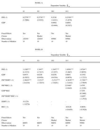
The results are reported in Table 1.4. In Panel A, specifications (i)-(ii), the earning yield is explained by the lagged month on month inflation rate. In all cases the estimated coefficient(INF) is positive and significant, implying that higher inflation drives real stock prices downwards. In order to control for the Fama proxy hypothesis, speci-fications (iii)-(iv) include the actual GDP growth rate in the following quarter13. The results show that inflation is still positive and
signif-icant, while the estimated coefficient for the expected growth proxy is positive but not significant. Note that in the last set of estimations the number of observations decrease substantially, from more than 126,000 to almost 70,000. The reason for this decrease in the number of observations is the lack of quarterly national accounts data14.
In Panel B of the Table 1.4, the effect of leverage on the inflation-stock price relation is tested.The variable DEBT is included in the model, which is the firm leverage (defined for the sector to which the firm belongs).
The model to be estimated is
13For the period data on the expected economic growth is not available. I use, as
a proxy, the actual GDP growth rate in the next quarter.
14Note that the sample for the second set of regressions is ”more recent” in time
than the previous set. To check if there is a sample bias when comparing both results, I repeat estimations (i)-(ii) using the same sample as in (iii)-(iv). The results hold, since inflation coefficient is still positive and significant.
E
Pi jt=α0+α1πjt−1+α2�gd pjt+α3πjtdebtjt+α4debtjt+ei jt
t=1, ...,T, j=1, ...,J, i=1, ...,I
wheredebtaccounts for the market debt to capital ratio, andπjtdebtjt
is the interaction term between inflation and leverage. The model is aimed to test if the stock price of firms with higher leverage should benefit from inflation, due to a decrease in the real debt value of the firm (α3 <0). The results in regressions (i)-(iii) show that the
leverage channel is significant. The coefficients for the cross term
INF*DEBT are negative and significant in the three regressions, im-plying that when inflation increases, real stock prices increase con-ditional on leverage. The coefficients for inflation are still positive and higher than in the Panel I estimations. Note that the inflation coefficients estimated in Panel A are the combination of both the co-efficients for inflation and for the interaction term of inflation and debt in Panel B.
Regressions (iv) and (v) in Panel B test whether there are asym-metric effects in economic expansions and contractions. I include a dummy variable (REC) taking the value one when GDP decreases and zero otherwise is included in the regressions. At a stock level, the asymmetric effect is not significant when including the leverage channel, sinceINF*REC is not significantly different from zero, im-plying no significant differences for the inflation-real stock price re-lation whether the economy is contracting or expanding.
The second panel specification, the market-portfolio specifica-tion, takes each market as the panel unit. The market earnings price is regressed on monthly inflation. In this case, the benchmark regres-sion is
E
where the dependent variable EP jt is the earnings yield corresponding to market j at timet; πjt−1 is the month on month inflation rate of
country j at time t−1; �gd pj,t is the following quarter real GDP
growth rate. Market dummy variables are included when noted. I also include the market debt over capital ratio and the cross-term of inflation times the debt ratio (to test the leverage channel).
In Table 1.5, the estimation results are reported. In specification (i), the inflation coefficient remains significant and positive. Thus, higher inflation correlates with lower stock prices. The leverage chan-nel is again significant. Conditional on the debt to capital ratio, higher inflation rate correlates with higher real stock prices. In models (ii)-(iv), I test if asymmetric effects are present. While for the stock approach there were not significant asymmetries, a different picture emerges when working with market earning yields. The results show that a relevant share of the variance is explained when the economy is contracting. When the economy is expanding, inflation coefficient is positive but not significant when the leverage channel is included (specifications (ii) and (iv)). Thus, most of the unconditional corre-lation between infcorre-lation and real stock prices is explained in contrac-tion periods, when both risk aversion and uncertainty are high. This last result is in line with the recent paper by Bekaert and Engstrom (2010). For the leverage channel, both during expansion and contrac-tion periods the coefficients are negative and significant, implying that inflation increases stock prices by decreasing real debt.
1.3.1.1 Real Stock Price, Inflation Level and Inflation Volatility
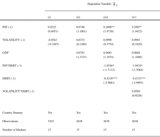
One potential explanation for the correlation between inflation and real stock prices is that it is inflation volatility, not the infla-tion level, what drives the correlainfla-tion. Higher inflainfla-tion volatility increases uncertainty, thus driving stock prices lower. In order to test if inflation volatility is indeed the relevant dimension in order to explain the correlation between inflation and stock prices, I
clude in the model specification inflation volatility as an indepen-dent variable (VOLATILITY). The series are estimated by fitting an AR(1)-GARCH(1,1) model to the monthly inflation series15.
Infla-tion condiInfla-tional volatility is included as an independent variable in the specification, in order to check if the inflation level remains to be significant.
The results from including inflation conditional volatility as an independent variable are presented in Table 1.6. In all specifications, the coefficient for inflation volatility (VOLATILITY) is not signifi-cant, and shows a positive sign, implying lower stock prices. How-ever, inflation level (INF) is positive in all specifications, but only sig-nificant when controlling for leverage. In specification (iv), the inter-action term of volatility and debt is included (VOLATILITY*DEBT), finding no significant effect. The conclusion is that it is the infla-tion level, not volatility, what drives the correlainfla-tion between earnings price ratios and realized inflation.
1.3.1.2 Asymmetric Crisis Effects
Another interesting dimension to analyze are the possible asym-metric effects when the economy is facing different crisis. Given the number of crisis-events in the EM sample, it seems almost naturally to test if the correlation experience significant changes when con-ditioning on crisis. I analyze the correlation of inflation and price-earning ratios for different crisis-typologies: currency, banking and twin crises. For that matter, the crisis dummy variable is interacted with the inflation rate (INF*CURR, INF*BANK, and INF*TWIN) and
leverage (INF*DEBT*CURR, INF*DEBT*BANK, and INF*DEBT*TWIN).
A currency-crisis starts in the month showing a significant increase in depreciation rate (vis-a-vis US dollar) and ends in the month in which depreciation peaks. For banking-crisis, the starting month is
15I also use this estimation setup to decompose realized inflation into its expected
taken from Laeven and Valencia (2008), and the ending month corre-sponds to the month in which banks deposits stabilize. Finally, twin-crisis months are those for which both currency and banking twin-crisis are observed.
The results are in Table 1.7. Column (i) presents the results from regressing earning yield on inflation, leverage and its cross-term for in all periods. Column (ii) shows the results for currency-crisis peri-ods, Column (iii) for banking-crisis, Column (iv) for twin-crisis and, finally, Column (v) for banking and currency crisis periods that do not correspond to twin-crisis months.
For all periods (first row of the estimations), inflation coefficient
(INF) is always positive and significant: higher inflation correlates with lower stock prices. The interaction term INF*DEBT, i.e.,
lever-age channel, presents a negative and significant coefficient in all five specifications: stock prices of more indebted firms increase when in-flation rises. Note thatDEBT shows a negative coefficient. Actually, this is true in the five specifications, but in all cases the coefficient is not significantly different from zero.
For currency-crisis periods, Column (ii), the conditional earning yield (Currency_crisis) is 0.0371 higher than during non-currency crisis periods, implying a 29.8 percent stock price decrease in annual-ized terms. The inflation coefficient for non-currency-periods (INF) is positive and very significant. For times of currency-crisis spell, an increase in the inflation rate correlates with a stronger decrease in the stock price (INF*CURR is highly significant). However, the effect is
minimized if the firm is leveraged. The interaction term of inflation and debt (INF*DEBT*CURR) presents a strongly significant negative
coefficient when currency-crisis months. Consequently, more lever-aged firms tend to net out the direct effect of inflation on stock prices. For banking-crisis periods - Column (iii) - the results show that when inflation rises, stock prices do not decrease more than in
banking-crisis periods. Both the interaction term between inflation and banking-crisis dummy(INF*BANK) and the interaction term be-tween inflation, leverage and the dummy(INF*DEBT*BANK) are not
significantly different from zero. This result is interesting when com-pared with the currency-crisis periods, where stock prices strongly decrease and leverage is key to understand which firms are more pun-ished by the market.
A potential caveat of the previous analyses is that for some peri-ods a country may suffer from both a currency- and a banking-crisis. In order to control for these particular periods, I define a twin-crisis as a period in which the country is suffering both types of crises at a time. The estimation in Column (iv) analyzes twin-crisis. Condi-tional on twin-crisis, the earning yield increases by 0.0508, implying a 36.5 percent stock price decrease in annualized terms. The results show that the effect of both currency and banking crises seems to net out, being the conditional effects of inflation not significantly different from those under non-twin-crisis periods (INF*TWIN and
INF*DEBT*TWINare not significant).
Finally, in Column (v), I analyze periods of non-contemporaneous currency and banking crisis. That is, crisis periods that are not twcrisis periods. First, note that the differential effect on both the in-flation and leverage effect for currency crisis is back in the picture. As in the analysis for currency crises in Column (ii), the interaction terms with the currency-crisis dummy(INF*DEBT*CURR) is strongly significant. The higher the leverage, the lower the stock price impact of inflation under currency crisis. Nota that for banking crisis periods this is not true, coherently with the findings in Column (iii).
1.3.2 Inflation and Real Earnings
downwards. If so, inflation at timetshould be able to forecast lower real earnings in the next periods. While empirical evidence does not support the assumption for developed markets, I directly test this real channel in the case of EMs. Again, both the stock and market-portfolio specification estimations are discussed16.
The results for the stock-approach are included in the first panel of Table 1.8. In the four specifications presented in the table, in-flation (INF) correlates negatively with real earning variations. The results are robust when including a trend variable, fixed effects, and clustering the errors. In the second panel of Table 1.8 the results for the market-portfolio regressions are presented17. Contemporaneous
as well as lagged inflation rates are always significant, with the only exception of two-month lagged inflation. The sign of the estimated coefficients is always negative: increasing inflation forecasts negative real earnings variations in the coming months. The estimated coeffi-cients are rather stable for the three quarters included in the regres-sions. These coefficients imply a decrease in real earnings between 0.18-0.40 percent per one percent inflation increase18. On average,
the inflation spell duration is about 12 months.
In Table 1.9, I test whether the relation changes if the economy is expanding or contracting. During contractions there is no significant differential effect of inflation on future real earnings, as INF*RECj
are no significant, for j=1, 2, 3, 6, and 9 lags. Consequently,
infla-16Concerns on using monthly variations are addressed by using quarterly data,
and year on year as well as quarter on quarter variations when working with earning growth rates.
17Results from the sector-portfolio approach are in line with the results presented
in this section.
18In Aizenman and Marion (2009) an inflation of five percent is associated with
an output cost during the inflation-disinflation cycle of about three percent of GDP for the US, which implies a cost of 0.60 percent on a monthly basis. The results for EMs show rather smaller implied inflation cost, between 0.18 and 0.40. While the comparison is not strictly correct, since one is measuring the impact on GDP and the other on aggregated earnings, both figures should be close, as in the present case.
tion drives real earnings growth rates downwards independently of the economic cycle. The estimated coefficients imply a real earn-ing decrease between 0.15 and 0.40, similar to the results in Table 1.8. Finally, I explore asymmetric effects of inflation on real earning variations when the economy is suffering different types of economic crises: currency, banking and twin-crisis. As before, a dummy vari-able is created for each type of crisis: Curr-Crisis, Bank-Crisis and
Twin-Crisis. The first part of Table 1.10 introduces the results for the crisis-conditional effects on real earnings growth rates. Note that Twin-Crisis is the strongest type of crisis, coherent with the effects of crisis on real stock prices. For currency-crisis, real earning growth rate decreases by 2.5 percent on a monthly basis; for banking-crisis 1.7 percent; and for twin-crisis 5.6 percent (26 percent; 19 percent; and 49 percent annualized decrease, respectively)19. Since crisis
pe-riods are contemporaneous to contractions pepe-riods, the results in Ta-ble 1.10 suggest that for the average crisis-period the correlation be-tween inflation and real earnings growth rates should not be signifi-cantly different from the non-crisis periods correlation. Coherently, in specifications (ix)-(xii), no significant differential effect is captured for the inflation-real earning correlation during crisis-months. None of the variablesINF*CURR, INF*BANK orINF*TWIN are signifi-cant. Inflation negatively affects real earnings, independently on the economic cycle and type of crisis. However, as discussed before, the correlation between inflation and real stock prices does vary in a different way conditional on the type of crisis. I find these results are indirect evidence supporting Beakaert and Engstrom (2010) claim that inflation correlates with higher risk aversion and uncertainty.
I conclude this section stressing the three main findings: i) there is a strong negative relation between inflation and future real earnings; ii) there is no significant difference when conditioning on the
nomic cycle (contractions and expansions); and iii) there is no signif-icant difference when conditioning on crisis-types (currency, banking or twin crisis). Given that the inflation-real stock prices correlation does vary in a different way conditional on the business cycle and type of crisis, the results in ii) and iii) are to be understand as indirect evidence for a positive relation between inflation and risk aversion (uncertainty).
1.3.2.1 Non-Linearities
The paper by Bruno and Easterly (1998) shows that the effect of inflation on GDP growth only becomes negative once inflation is above a threshold level of 40 percent on an annual basis. This non-linear relation can be analyzed with more rigor since Hansen (2000, 1999) introduced panel threshold model estimation. In the studies that followed, the results show that below the threshold there is no significant relation between inflation and GDP growth rates, while above the threshold there is a robust negative relation20.
In this paper, I am interested in testing if there is a significant threshold for the inflation - real earning growth relation. That is, if existsπ, such that whenπt<πthe correlation is not significant.
Fol-lowing Hansen (2000), a threshold panel estimation is performed. For real earnings growth rates the model to estimate is
�reit=αi+β1�πitI(πit≤π) +β2�πitI(πit>π) +β3��GDPi,t−1+εit 20A number of papers have analyzed the relation between inflation and GDP
growth using threshold models. Drukker et al. (2005) use a non-dynamic, fixed effects panel data framework to analyze the correlation for 138 countries in the period 1950-2000. For the full sample, they find a threshold inflation level of 19.2 percent. Below this level, there is no significant effect of inflation on growth. Above the threshold, inflation correlates negatively with GDP growth rates. Khan and Senhadji (2001) find similar results, but for a balanced panel. For industrialized countries the threshold is between 0.89-1.11 percent inflation level, while for non-industrialized 10.62-11.38 percent. Using a dynamic panel approach, Kremer et al (2009) find a 2 percent threshold for industrialized and 17 percent threshold for non-industrialized.
where�reitis the capital weighted real earning growth rate of market iand montht ; πit is monthly inflation rate;�GDPis the real GDP
growth rate, andπis the threshold inflation rate to be estimated. Following the steps described in Appendix 1.1, I first find the threshold point estimation, which is 0.007452 (9.32 % annualized rate). Second, the model estimation is repeated, but differentiating with a dummy variable the effect of inflation being below or above the estimated threshold. The results are in Table 1.11. Column (i) shows the results when no threshold is assumed. Column (ii) shows the results for the estimation incorporating the threshold inflation rate. For that, two dummies are included in the specification, one having value 1 when πt < π and 0 otherwise, and the other having value
1 whenπt >π and 0 otherwise. Note that when inflation is below
or above the estimated threshold does not change the main results in the paper: either below or above the threshold, higher inflation correlates with lower real earnings growth rates. The conclusion from the threshold panel analysis is that inflation does correlate negatively with real earnings growth rates, independently of the inflation level. Thus, the results in previous sections do not suffer from any of the biases emphasized by the threshold-panel literature21.
1.3.2.2 Quantifying the impact of decreasing real earnings growth rates on real stock price variations
Quantifying the impact of inflation on real earning growth rates allows explaining the actual variation in real stock prices when fac-ing an inflation shock. Specifically, I estimate the share of the real stock price variation explained by inflation only affecting real earn-ing growth rates. A simple way to estimate the share of the real stock price variation that is explained by inflation only affecting real
earn-21It’s worth to emphasize that I am working with a special type of firm, since
ings growth rates is to multiply the estimated coefficients coming from: i) regressing real stock prices on real earnings growth rates; and ii) regressing real earnings growth rates on inflation. The results from different specifications show that estimated share is between 18 and 20 percent. In other words, inflation only decreasing real earnings growth rates explains a fifth of the variation of the real stock price. Similar results are found when calibrating asset-pricing models to the EM sample.
The question then is what factors may explain the 80 percent of the real stock price variation that is not explained by decreasing real earnings growth rates. Bekaert and Engstrom (2010) find that, in the case of the US, the positive relation between inflation and risk explains almost half of the variation of the real stock price when fronting an inflation shock. Assuming this figure as a floor for EMs, then the room left unexplained is reduced to less than 30 percent. This implies that the room for money illusion in EMs is substantially less than in the case of developed markets. This seems puzzling, since developed markets are deeper, more liquid and transaction costs are lower than in EMs. In this case, non-arbitrage conditions seem more sensible in developed markets than in EMs, preventing recurrent val-uation errors to exist. On the other side, it can be argued that the cost of inflation related valuation errors may be higher in EMs than in de-veloped markets, which may explain the more extended presence of money illusion in developed countries.
1.4 S
ECTOR
A
NALYSIS
Two empirical questions can be answered when working with sector-portfolios: a) which sectors perform better as inflation hedges; and b) which sectors present higher earning resilience to inflation. In the case of EMs, I find that some sectors showing strong earnings re-silience to inflation are nonetheless punished by the market as their
real stock prices fall; while some sectors showing strong earning de-creases are nonetheless good hedges against inflation, as their real stock prices do not fall and in some cases they even increase.
In Table 1.12, I present the future 12-month real earning growth rate variations and the monthly earning yield variation conditional on a five percent annualized inflation shock, for the most aggregated sec-tor classification (10-secsec-tor aggregation). The only secsec-tor experienc-ing a 12-month increase in real earnexperienc-ings growth rates is Telecommu-nications. As expected, the earnings price variation presents a neg-ative value implying an increase in the sector real stock price. The rest of the sectors present negative real earning variations and lower real stock prices (positive earning yield variation), with the notable exception of Utilities. For Utilities, stock prices increase even though earnings growth rates decrease. Therefore, in EMs, an index follow-ing Utilities seems to be the best stock market hedge against inflation. In Figure 1.2, the variation in the future 12-month earning growth rate and the variation in the earning yield is plotted for the 60 sectors available at the lowest aggregation level. Again, a positive varia-tion in the earning yield indicates a decrease in stock price. As ex-pected, most of the sectors experience both a decrease in stock prices and real earnings due to inflation (sectors included in the quadrant IV). Telecommunication sub-sectors are the ones plotted in quadrant II (increasing earnings and real stock price). The sectors included in quadrant III present increasing stock prices and decreasing real earnings. The second part of Table 1.12 shows those sectors with increasing stock prices and decreasing real earnings. As expected, most of these are subsectors of Utilities. Note that Water Utilities and Wireless Communication Services have their stock prices increasing eventhough inflation severely punishes their earning growth rates.
prob-lem is that most of these sectors are very small, with capitalization lower than one percent of the market. In order to control for very small sectors driving the results, in the second panel I only include sectors with capitalization higher than one percent. In this case, only two sectors present both an increase in prices and earnings: Marine and Multi-Utilities. Again, the capitalization of these two sectors is barely above the one percent threshold (1.4 and 1.1 percent), so other issues may be playing a big role in the correlations.
1.4.1 Sector-Portfolio Specification
In this section, I go through the results when working with the sector-portfolio specification. While the main results still apply, there is a new dimension to discuss in relation to the leverage channel. I find that the leverage channel is robust for big sectors, but not for small sectors. I conjecture that small sectors suffer more financial constraints than big ones, and therefore the effect for small sectors is not found to be significant.
The benchmark regression when working with sector-portfolios is
E
Pk jt=α0+α1πjt+α2�gd pj,t+1+α3πjtdebtk jt+ ...+α4debtk jt+µk+ζj+ek jt
t=1, ...,T, k=1, ...,K j=1, ...,J
where the dependent variableEP k jt is the earnings yield corresponding to sectork of market j at timet, πjt is the month on month inflation
rate of countryjat timet;gd pj,t+1in next quarter actual GDP growth
rate;debtk jt accounts for the market debt to capital ratio for sector k
of country jat timet, andπjtdebtk jt is the interaction term between
inflation and leverage. Fixed effects at a sector and market level are included when noted. A long panel estimation is performed, since
the number of time periods is higher than the number of cross-section units. The results are reported in Table 1.13, which is divided in three panels. Panel A shows the benchmark specification adding a trend variable to control for common time effects. The estimated inflation coefficient is positive and highly significant, as expected. In Panel B, I control for the Fama proxy hypothesis by including next quarter real GDP growth rate. At a sector level, positive variations in next quarter GDP are associated with higher stock prices. The inflation coefficient remains positive and significant, when including next quarter GDP growth rate.
Finally, in Panel C, the leverage channel is tested. When including in the panel estimation the sector leverage variables, the estimated coefficients for inflation and next quarter economic growth rate do not show differences with the previous results, but the coefficient for the cross term of inflation and leverage presents a puzzling positive sign. This implies that the higher the firm leverage, the more the stock price decreases when inflation jumps. This result seems puzzling, in particular when we find a strong and robust positive effect when dealing with individual stocks and market earning yields. The main difference is that we are imposing an equal weight on each sector in the sector-portfolio panel estimation. That is, a small sector in Argentina weights the same as a big sector in the same country. When working with market earning yields this is not a problem, since capital weights are used to construct the dependent variable.
In order to test if big and small sector asymmetries are behind the results, the following specification is estimated
E
Pk jt =α0+α1πjt+α2�gd pj,t+1+α3πjtdebtk jt+ ...
t=1, ...,T, k=1, ...,K j=1, ...,J
where the dependent variableEP k jt is the earnings yield corresponding to sectorkof country jat timet(weighted by firm capitalization). πjt
is the month on month inflation rate of country jat timet;gd pj,t+1in
next quarter actual GDP growth rate;πjtdebtk jt is the cross-product
of inflation times the sector leverage; and�Capk jt−Capjt� is a weighting
term denoting sectork capitalization minus the average sector capi-talization of country jat timet. Fixed effects at a sector and country level are included when noted.
Including the sector weight�Capk jt−Capjt�allows separating the
lever-age effect for big sectors (sectors which capitalization is above aver-age) and small sectors (sectors which capitalization is below averaver-age). The results presented in Table 1.14 show that sector asymmetries are significant. When introducing sector country dummies -columns (iv) and (v)- the coefficient for the termπjtdebtk jt�Capk jt−Capjt�
be-comes negative and significant. Moreover, the estimated coefficient for the termπjtdebtj is negative but not significant. From the model
specification, the leverage effect can be decomposed as:
∂2E P
∂π∂debt = α3+α4
�
Capk jt−Capjt� (1.1)
Note that you can read the first term -α3− as the coefficient for
the average sector, being the average sector the one with capitaliza-tion equal to the average of all the sectors�Capk jt=Capjt�. Therefore, for
the average sector the leverage impact is not significant. However, for big sectors the leverage channel is significant. The same is not true for small sectors (those below the average sector capitalization). In Figure 1.3, I plot the estimated impact of a one percent inflation rate on the earnings price, conditional on the capital weight of the sector as in Equation 1.1. For a sector above average, the effect is
tive and significant, implying an increasing stock price for firms with higher leverage. On the other side, for sectors close to the average or below the average, the leverage effect is positive and non significant. Under the sector-portfolio approach, I conclude that the leverage channel is present: higher inflation increases stock price conditional on firm leverage. However, the result does not hold for all the sec-tors, but for the big sectors. These are the ones that show a positive correlation of inflation on stock prices conditional on indebtedness. I conjecture that small sectors suffer more financial constraints than big ones, and therefore the effect for small sectors is not found to be significant. While there is a empirical evidence supporting this claim for developed markets, there is not evidence for EMs as an asset class. I leave testing this conjecture for future research.
1.5 D
ISCUSSION AND
C
ONCLUSIONS
In this paper I provide new insights into the effects of inflation on real stock prices. Since the seminal work of Modigliani and Cohn (1979), the majority of papers have emphasized behavioral factors. I test the different real channels suggested in the literature in the case of EMs, and find strong empirical support for all of them. The results support Friedman’s claim that inflation imposes real economic costs, and at the same time questions the need to build on money illusion and related approaches.
evi-dence of non-linearities in the inflation-earning growth rate relation. The results are robust to aggregation methods and data frequencies.
Second, there is a positive relation between inflation, risk aver-sion and uncertainty, as suggested by Bekaert and Engstrom (2010a). This channel is tested in an indirect way. First, I show that the rele-vant share of the explained variance driving the inflation-stock price correlation takes place in contraction periods. Since risk aversion and uncertainty are higher during recessions, these results can be taken as indirect evidence of the positive relation between inflation and risk aversion (uncertainty). Second, I show that the relation be-tween inflation and real earnings growth rates does not show signifi-cant asymmetries conditioning on crisis-types: currency, banking and twin-crisis. However, the earning yield does show asymmetric re-sponses conditioning on the type of crisis. As before, I interpret these results as inflation affecting risk quantity and risk price.
Under imperfect capital markets inflation may affect real stock prices in a positive way. As suggested by Ritter and Warr (2002), in-flation affects equity values by decreasing the real value of corporate debt. For a given expected real cash flow (i.e. firm value), inflation decreases the real value of debt, increasing the equity value and thus driving stock prices upwards. The results show that this real channel, the leverage channel, plays a significant role in EMs. Higher inflation increases stock prices conditional on sector indebtedness. At a sector level, the evidence shows that the more indebted the sector, the higher the impact of inflation on the equity price, but the effect is not signif-icant for small sectors. This is consistent with firms in small sectors suffering more from financial constraints than firms in big sectors.
In order to gain further insights into the mechanisms driving the relation between inflation and real stock prices, I explore which sec-tors are the best hedges against inflation, and which secsec-tors present highest earning resilience to inflation. Interestingly, the results show
that some sectors present strong earning resilience to inflation but are nonetheless punished by the market, while some sectors that show strong earning decreases are good hedges against inflation. The fac-tors explaining these sector asymmetries are left for future investiga-tion.
The evidence for real channels in the EM sample allows dis-cussing the room for money illusion when explaining the negative correlation between inflation and real stock prices. Inflation decreas-ing real earndecreas-ings growth rates accounts for 20 percent if the real stock price variation. While in this paper I do not quantify the importance of the other two real channels, we can draw upon the literature for the risk channel. Bekaert and Engstrom (2010) show that, for the US, the inflation-risk relation explains up to 50 percent of the real stock price variation. Therefore, there is less room for money illusion in EMs than in developed markets, what seems to be a puzzling result.
Figure 1.1: Emerging Market Monthly Inflation Average
Notes: The figure shows average month on month inflation rates (seasonally adjusted). The 1st (in blue), 2nd (in red) and 3rd (in green) quartiles are plotted on the left axis. The 4th quartile (dotted line) is on the right axis. During the 80s, inflation monthly inflation was high and volatile (Great Inflation). After mid-90s, inflation decreased considerably and has remained low and stable since then.
Emerging Market Monthly Inflation Average monthy figures (annualized figures in parentheses)
1985-2007 1985-1990 1990-2000 2001-2007 Mean 0.01977 (0.2684) 0.05633 (0.9302) 0.017959 (0.2381) 0.00509 (0.0628)
Volatility 0.06576 (0.2278) 0.13887 (0.4811) 0.04555 (0.1578) 0.00686 (0.0237)
Skewness 12.02 8.19 5.43 4.83
Kurtosis 236.9 96.56 36.23 42.75
Figure 1.2: Earning Yield Variation and 12-Month Real Earning Growth Rate Variation
Notes: The figures show the estimated variation of earnings yield (monthly variation) and real earnings growth rates (12-month variation) given a 5 percent inflation shock. The horizontal axis plots the earn-ing yield change, while the vertical axis the change in real earnearn-ings growth rates. Note that positive variations in earning yields imply a decrease in the stock price. Sectors with positive earnings growth rates and increasing stock prices are plotted in quadrant I; sectors with increasing earnings and real stock price in quadrant II; sectors with increasing stock prices and decreasing real earnings in quadrant III; and sectors with negative real earnings and decreasing stock prices in quadrant IV. The upper panel shows 60 sectors, while the lower panel shows only those sectors which capitalization is above one percent of the market capital.
60-Sector Aggregation
(earnings yield variation is plotted on horizontal axis while change in real earnings growth rates on vertical axis)
60-Sector Aggregation: Capitalization higher than one percent
Figure 1.3: Leverage Effect and Sector Capitalization
Notes: The figure plots the leverage effect of inflation over earning yield, as described below. The horizontal axis shows the sector capital weights�Capk jt−Capjt�. A positive effect implies a decrease
in the stock price, while a negative figure implies an increase in the stock price. In the figure I plot the estimated impact of a one bps inflation rate on the earnings price, conditional on the leverage. Following the model in Eq (9), the leverage effect is: ∂2
e p k jt
∂π∂Debt=α3+α4�Capk jt−Capjt�. Note that
you can read the first term -α3−as the coefficient for the average sector, being the average sector the one with capitalization equal to the average of all the sectors�Capk jt=Capjt�. The figure is done using the
estimation in Table 4.2, column (v). For a sector above the average, the effect is negative and significant, implying an increasing stock price for firms with higher leverage. On the other side, for sectors close to the average or below the average, the leverage effect is positive and non significant.
Table 1.1: Emerging Market Capitalization
Notes: the figures correspond to the sample average. Nominal exchange rates were used to translate capital from domestic currency into dollar denominated. The share is calculated over the 24 countries included in the EMDB database, of which due to data issues I end up working with 15 countries.
Country Share
Korea 13.9%
Brazil 9.2%
India 9.1%
Malaysia 5.5%
Mexico 5.3%
Chile 2.7%
Turkey 2.5%
Poland 1.9%
Argentina 0.9%
Peru 0.8%
Egypt 0.8%
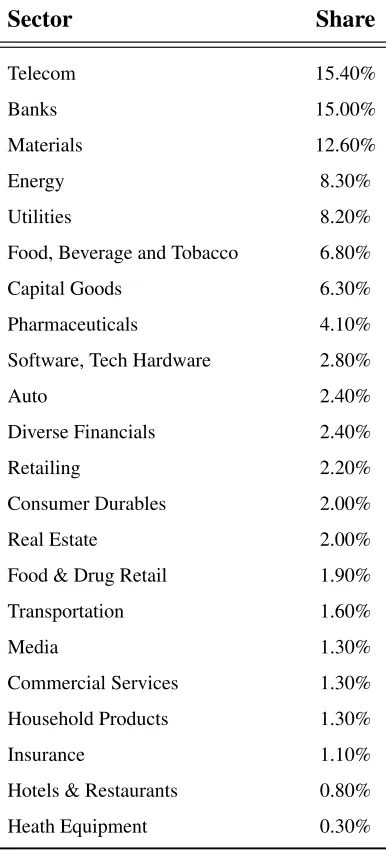
Table 1.2: Sector Capitalization
Notes: the figures correspond to the sample average. Nominal exchange rates were used to translate capital from domestic currency into dollar denominated.
Sector Share
Telecom 15.40%
Banks 15.00%
Materials 12.60%
Energy 8.30%
Utilities 8.20% Food, Beverage and Tobacco 6.80% Capital Goods 6.30% Pharmaceuticals 4.10% Software, Tech Hardware 2.80%
Auto 2.40%
Diverse Financials 2.40% Retailing 2.20% Consumer Durables 2.00% Real Estate 2.00% Food & Drug Retail 1.90% Transportation 1.60%
Media 1.30%
Commercial Services 1.30% Household Products 1.30% Insurance 1.10% Hotels & Restaurants 0.80% Heath Equipment 0.30%
Table 1.4: Inflation and Real Stock Prices: Stock Specification
This table reports a panel estimation to test the effect of monthly inflation on real stock prices. The dependent variable is the monthly earnings price ratio for each stock traded in the Emerging Market sample. Independent variables are: INF is the monthly inflation rate; GDP is the next quarter actual GDP growth rate, as a proxy for expected growth. DEBT is a variable that controls leverage, the debt to capital ratio (mark to market), from Bloomberg. See Section 2 for construction of the leverage series. INF*DEBT is the cross-product of INF and DEBT variables. The table reports point estimates with t-statistics (in parentheses) clustered as described in the Cluster row. Country dummy variables, and fixed effects added when noted. ***p<0.01, **p<0.05, *p<0.1. The sample period is January 1986-December 2007.
PANEL A
Dependent Variable:EP i jt
(i) (ii) (iii) (iv)
INF(-1) 0.2770*** 0.2770*** 0.2158 0.2158*** (3.3806) (2.9252) (1.6211) (3.4570)
GDP 0.0984 0.0984
(0.4446) (0.1927)
Fixed Effects Yes Yes Yes Yes
Cluster - Market - Market
Observations 126303 126303 69966 69966
Number of Markets 15 15 15 15
PANEL B
Dependent Variable:EP jt
(i) (ii) (iii) (iv) (v)
INF(-1) 1.1305*** 1.3447* 1.3447*** 1.4956*** 1.8744** (4.3333) (1.7413) (3.3257) (3.2667) (3.0039)
GDP 0.0975 0.0250 0.0250 0.0051 -0.5392
(0.3852) (0.0450) (0.0354) (0.0076) (-1.7233) INF*DEBT (-1) -2.8618*** -3.1513* -3.1513*** -4.3639*** -5.7301**
(-4.6310) (-1.9215) (-3.0281) (-3.4442) (-2.9049)
INF*REC (-1) 0.3440* 1.4795
(1.8442) (1.3156)
GDP*REC 3.7255
(0.7408)
INF*DEBT*REC (-1) -3.6497
(-1.2516)
DEBT (-1) -0.1276 - - -
-(-1.0276) . . . .
REC (-1) -0.0126 -0.0056
(-0.6459) (-0.3926)
Fixed Effects Yes Yes Yes Yes Yes
Cluster - - Market Market Market
Observations 60652 60652 60652 60090 59984