How important is access to employment offices in Spain? An urban and non urban perspective

Texto completo

(1)© Investigaciones Regionales. 21 – Pages 119 to 140 Section Empirical contributions. How important is access to employment offices in Spain? An urban and non-urban perspective Patricia Suárez Cano*, Matías Mayor Fernández*, Begoña Cueto Iglesias*. ABSTRACT: The aim of this paper is to analyze the effect of the accessibility to employment offices on local unemployment rates according to the distribution of three different types of municipalities: large urban, small urban and non-urban. We built a new accessibility measure taking into account the number of employment offices together with the distance and size of their catchment area. We propose an empirical model with spatial regimes that allows including simultaneously spatial heterogeneity and spatial autocorrelation. The results suggest that the accessibility to employment offices is especially important in non-urban areas where employment opportunities are limited. Employment services are important because bridge the gap between unemployed workers and employers where job opportunities are unclear. JEL Classification: J68, C21, R12. Keywords: Accessibility, employment services, spatial autocorrelation, spatial he terogeneity, spatial regimes.. ¿Importa el acceso a las oficinas de empleo en España? Un análisis por tipo de municipio: urbano vs no urbano RESUMEN: El objetivo de este trabajo es analizar el efecto de la accesibilidad a las oficinas de empleo sobre la tasa absoluta de paro teniendo en cuenta la relación de cada municipio con el fenómeno urbano, es decir, si pertenecen a grandes áreas urbanas, a pequeñas áreas urbanas o a áreas no urbanas. Se ha construido un índice de accesibilidad teniendo en cuenta el número de oficinas de empleo, la distancia desde cada municipio al municipio en el que se encuentra la oficina de empleo de referencia y el tamaño del mercado de trabajo de cada oficina de empleo. Se ha estimado un modelo que distingue estos tres tipos de regímenes espaciales incluyendo de forma simultánea la existencia de autocorrelación y heterogeneidad espacial. * Applied Economics Department, Faculty of Economics and Business. University of Oviedo. Corresponding author: Matías Mayor, Applied Economics Department, Faculty of Economics and Business, University of Oviedo, Oviedo (33006), Spain. E-mail: [email protected]. Received: 19 may 2011 / Accepted: 06 september 2011. 119. 08-SUAREZ.indd 119. 24/2/12 09:25:59.

(2) 120. Suárez, P., Mayor, M. and Cueto, B.. Los resultados sugieren que la accesibilidad a las oficinas de empleo es especialmente importante en las áreas no urbanas donde las oportunidades de empleo son más limitadas y confusas. Clasificación JEL: J68, C21, R12. Palabras clave: Accesibilidad, servicios de empleo, autocorrelación espacial, heterogeneidad espacial, regímenes espaciales.. 1.. Introduction. Regional labor market disparities in Spain are rather large and persistent; hence they must be addressed in active labor market policies (ALMPs). The decentralization of ALMPs has greatly changed the legislation governing the institutional structure of the labor market over the last decade. At present, local employment offices under regional public employment services are responsible for the implementation of active programs. Therefore labor market policies have become a central concern in Spain and politicians have started to recognize the need for further evaluation to assess their current state. The resources in terms of the number of employment offices are not uniform across autonomous communities and, consequently, some are doing better than others. With respect to the Public Employment Service (PES), in theory it provides jobseekers easy access to employers and labor markets at local, regional, national and European level. Placement services are located in space, hence analyses of the accessibility to employment offices require spatially explicit tools. Also, any improvements in accessibility would translate into better PES performance, so we need to discuss whether the accessibility to employment offices is really equitable regardless of place of residence. Also, recent planning, evaluation and policy analysis have devoted more attention to accessibility measures. This paper focuses on the spatial distributions of unemployed workers and public employment offices in Spain. Clearly, the distribution of public employment offices in the territory may lead to differences in accessibility for the unemployed and, in turn, have effect on the PES performance. Studies on the efficiency of PES offices at local level have been done in Germany (Hagen, 2003), Switzerland (Sheldon, 2003) and Sweden (Althin and Behrenz, 2004). However, these studies have not analyzed whether the spatial distribution of employment offices ensures equal access to such offices. In Spain there are no studies of employment offices at local level and, as in other countries (Fertig et al., 2006), we do not know how public funding is distributed among the offices. The aim of this paper is twofold. First we present a new approach for tackling differences in access which combines the methodology of spatial methods with new accessibility measures that take into account the size of an employment office catchment area. Second we explore whether the spatial heterogeneity shown in several. 08-SUAREZ.indd 120. 24/2/12 09:25:59.

(3) How important is access to employment offices in Spain? An urban and non-urban perspective 121. studies, viz. that labor market problems in large cities greatly differ from those in non-urban areas, may have a substantive interpretation in the sense that different spatial regimes apply for different types of municipalities. The outline of the paper is as follows: Section II describes the data used in the paper and examines basic features of the unemployed and employment offices in relation to the different types of municipalities existing in Spain. It also introduces the accessibility measures proposed. In Section III we estimate an unemployment rate equation which includes the accessibility to employment offices as explanatory variable. Section V concludes with some policy recommendations.. 2.. Data and methodology. 2.1. Data. Unemployment data in the following pages have been taken from the Official Unemployment Statistics, which are published monthly by the SPEE. Data refering to the local employment offices and their catchment areas have been taken from the regional employment authorities websites and the SPEE website. It is essential to establish clusters of unemployed people at local level, since active job-seeking policies and the modernization of PESs should be more intense in such municipalities. Figure 1 shows the spatial distribution of employment offices in Spain. Clearly, its most striking feature is the large number of municipalities lacking employment offices –7,524 out of 8,109. Figure 1. Employment office location (2009). Source: own elaboration.. 08-SUAREZ.indd 121. 24/2/12 09:25:59.

(4) 122. Suárez, P., Mayor, M. and Cueto, B.. The many municipalities with zero employment offices are predominantly concentrated in Castile and Leon, whereas the nonzero ones are in the south and the south-east, Madrid and Barcelona. Notwithstanding that, the data shows employment offices in every municipality with over 4,000 jobless, except Paterna and Mislata (Valencia metropolitan area), San Vicent del Raspeig (Alicante metropolitan area), Mijas (Malaga) and Los Realejos (Tenerife). Graph 1 shows the existence of steep differences between the Spanish autonomous communities in the number of unemployed workers per employment office. The number of employment offices seems to be far below the number of jobless they have to attend to, especially in Madrid, the Canary Islands, the Valencian Community and Catalonia, so differences in accessibility may be expected. Graph 1. Average number of unemployed workers per placement office. NUTS-II (2009). Source: own elaboration.. 2.2. Measuring accessibility. Several authors from different perspectives have analyzed the concept of accessibility within the framework of urban and regional economies. For instance, Krugman (1991) and Fujita et al. (1999) study the importance of accessibility in economic development from a regional perspective. Most existing studies on accessibility belong to the field of transportation economy. Gutierrez (2001) and Holl (2007) analyze accessibility improvements in Spain. From a theoretical perspective, Geurs and Van Wee (2004) review is remarkable for its analysis of the usefulness of accessibility measures in the evaluation of changes in transportation infrastructures and its use by researchers and policy makers alike. With respect to labor markets, accessibility measures are given consideration in few works. For instance, Van Wee et al. (2001) develop a concept of accessibility to analyze whether jobs are accessible for employ-. 08-SUAREZ.indd 122. 24/2/12 09:26:00.

(5) How important is access to employment offices in Spain? An urban and non-urban perspective 123. ees. Détang-Dessendre and Gaigné (2009) study the impact of the place of residence on unemployment duration. They rely on an accessibility measure to convey workers’ competition for jobs and subsequently tackle labor market tightness. JoassartMarcelli and Giordano (2006) use a geographic information system to look into the location of One-Stop Centers in Southern California and their level of accessibility. Consequently, their research is closely related to ours. As far as we know, in Spain there is no research on the spatial distribution of employment offices and their levels of accessibility. It is currently intended that active employment policies become an asset in the fight against unemployment so that assurance of equal access to employment offices is essential. We may begin by stating that, even though employment offices are administrative units that were created long ago, their spatial distribution is by no means random. However, regardless of the fact that it does follow a pattern, such distribution may cause either equity or inequity of access to the offices. Accessibility conditions should be the same regardless of the autonomous community of residence —whose government, in turn, is responsible for the administration of the employment offices. In other words, every unemployed worker should be equally treated, no matter where they may live. Talen and Anselin (1998) analyze the accessibility measures from a methodological point of view and take into account the spatial dimensions of equity. The simplest measure to analyze job-seeker accessibility to employment offi ces consists in counting the existing employment offices within a given area. Suárez (2011) developed a range of accessibility measures to employment offices, so this work relies on one of these accessibility measures, considered like the best option. This measure takes into account the number of employment offices together with the distance and size of their catchment areas. Consequently, the proposed accessibi lity measure is more empirically adequate, since some employment offices attend to approx. 20,000 jobless —e.g. Fuenlabrada (Madrid)—, whilst others attend to just 1,000 jobless —e.g. Caudete (Albacete)—. The accessibility to employment services is determined by this fact and that cannot be overlooked. We would like to have had access to the number of job counselors and/or counseling sessions per unemployed worker, but access to this information is not provided at local level. This measure is based on the number of employment offices per unemployed worker within a catchment area, adjusted for the distance between the municipality i and its corresponding employment office    EOj − λdij  − λd Ai =  ( e ) → Ai = w j (e ij )   ui ∑  ∈ i j  . (1). where Ai is the municipality accessibility, wj is the number of employment offi ces (EOj) per employment office catchment area (∑ ui), measured as the number i=j. 08-SUAREZ.indd 123. 24/2/12 09:26:00.

(6) 124. Suárez, P., Mayor, M. and Cueto, B.. of unemployed workers in the municipalities i within a single catchment area. Finally, dij is the distance between a municipality i and its corresponding employment office, and l is a parameter of the distance-decay function. This parameter determines the degree of interaction between the place of residence of the jobless and the employment office they have to go to, the accessibility quality decreasing as distance to the office increase. Even though several values were used for this parameter in Suárez (2011), the performance of a sensitivity analysis led us to set l = 0.10. The study of the internal accessibility or ‘self-potential’ of employment offices presents further problems, since there are no data on the exact distance to the office when job-seekers are assigned an office within their municipality of residence. Even though this problem has been studied by some authors (Bröcker, 1989; Frost and Spence, 1995), it remains unsolved in the literature. One option consists on the estimation of the internal distance using the formula proposed by Zwakhals et al. (1998) which is based on the surface of the municipalities considered 1. Since these municipalities are very similar (73% of the municipalities lacking employment offices are located in urban areas), another alternative is to assign the same distance value to such municipalities. Gutiérrez-i-Puigarnau et al. (2011) applies a similar solution to that of ours in the assignment of daily commuting distances for workers who commute to workplace locations within their municipality of residence. In our study, the first option rendered the results unreliable, so we imputed a value of 1 km for these municipalities (7.2% out of total), once the distribution of dij had been considered. 2.3. Municipalities classification. Before discussing in detail the classification of municipalities, we must examine the classification properties themselves. Graph 2 shows the classification of Spanish municipalities developed by the Department of Public Works 2, which has established Graph 2. Type of municipality. NON-URBAN AREA 7,055 (87%). URBAN AREA 1,054 (13%). Large urban area; 744. Small urban area; 310. 1 2. 08-SUAREZ.indd 124. (. ). di = 2 surfacei 3 . This classification is currently under review following the Population Name Index 2009.. 24/2/12 09:26:00.

(7) How important is access to employment offices in Spain? An urban and non-urban perspective 125. three different types of areas, viz. large urban, small urban and non-urban, according to their degree of urbanization. This classification has been built using data from the Population and Housing Census 2001, which have in turn been supplemented by more up to date information from the Population Name Index 2006. Both have been used as sources because they provide larger amounts of data at local level. Generally it has been established that every large urban area must include one municipality with a population of at least 50,000 inhabitants. Any other municipality within the same area should have a minimum of 1,000 inhabitants. In total there are 83 large urban areas in Spain (744 municipalities, 9.2% out of total), of which 19 comprise just one municipality and the remaining 64 comprise more than one. 310 municipalities (3.8% out of total) belong to small urban areas. On the whole, urban areas add up to 1,054 municipalities (13% out of total). They also account for about 80% of the total population and 20% of the surface area of the country. Non-urban areas comprise 7,055 municipalities (87% out of total). The main purpose of the classification is to identify differences between employment offices at regional level, so Graph 3 shows the classification of employment offices by type of municipality. In effect, 73% of the employment offices are located in urban areas. However, the distribution of employment offices differs across autonomous communities. Thus, Madrid, Catalonia and the Valencian Community have Graph 3. Classification of employment offices by type of municipality. Source: own elaboration.. 08-SUAREZ.indd 125. 24/2/12 09:26:01.

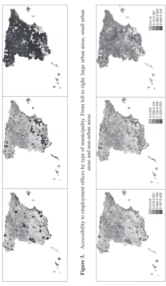
(8) 126. Suárez, P., Mayor, M. and Cueto, B.. 98%, 74% and 64% of their employment offices located in municipalities within large urban areas, respectively. Other autonomous communities such as Extremadura, Castile-La Mancha and Castile and Leon have about 50% of their employment offices in municipalities which do not belong to either large or small urban areas. It may naturally be expected that this fact has effect on job-seeker access to employment offices. We should bear in mind that employment offices, like ALMPs, have been transferred to the autonomous communities so that regional PES are responsible for the administration of both employment offices and a broad range of active labor market policies. The three maps in Figure 2 show the classification of municipalities according to their degree of urbanization, as previously mentioned. Then the three maps in Figure 3 show the distribution at local level of the accessibility variable for large urban areas, small urban areas and non-urban areas, respectively. The conclusions we get from these maps are in accordance with what was expected. Thus, whereas the differences between non-urban areas are quite significant, those between urban areas are less so. Notwithstanding that, we may further remark that some large urban areas (e.g., central Asturias; Badajoz, Caceres and Merida; Vigo-Pontevedra) show high degrees of accessibility. Also, the quite significant differences between non-urban areas bear out the importance of the distribution of employment offices and the definition of their catchment areas. Since generally employment offices located in municipalities within non-urban areas are the least crowded, accessibility is higher in such municipalities and, consequently, it may be expected that access to employment offices reduces local unemployment rates, especially in municipalities with limited employment opportunities (i.e., training and job placement). In non-urban municipalities, the benefits from having access to an employment office may be greater. 2.4. Spatial autocorrelation. Within the field of labor market studies, several contributions have taken into account the spatial dimension of regional labor markets and pointed out the high degree of interdependence of local labor markets (Molho, 1995; Lopéz-Bazo et al., 2002; Overman and Puga, 2002). Furthermore, Patacchini and Zenou (2007) analyze the reasons for the spatial dependence in local unemployment rates. This spatial autocorrelation is mainly due to the fact that the unemployed may seek and find work in different areas, so spatial interactions result from the mobility of the unemployed. When the data is collected at the administrative level, spatial autocorrelation is likely to be a relevant issue. This paper adds consideration of spatial dependences in local unemployment rates to the diverse influences exerted by public employment services across different levels of accessibility. A spatial analytical perspective is also recommended by Tsou et al. (2005) to evaluate suitability of urban public facilities in assessing whether or not, or to what degree, the distribution of urban public facilities is equitable. Notwithstanding that, not only is the spatial pattern of the offices relevant, but more complex aspects must also be taken into account, such as those relating to the. 08-SUAREZ.indd 126. 27/2/12 10:01:24.

(9) 08-SUAREZ.indd 127. Source: own elaboration.. Figure 3. Accessibility to employment offices by type of municipality. From left to right: large urban areas, small urban areas and non-urban areas. Figure 2. Types of municipalities. From left to right: large urban areas, small urban areas and non-urban areas. How important is access to employment offices in Spain? An urban and non-urban perspective 127. 24/2/12 09:26:02.

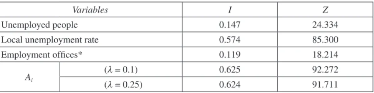
(10) 128. Suárez, P., Mayor, M. and Cueto, B.. accessibility indices calculated. Ideally, accessibility to employment offices should be kept at an adequate level even in high local unemployment rate contexts —in other words, there should be no municipalities with low accessibility levels. This section examines global spatial autocorrelation in local unemployment rates, employment offices and accessibility measure. Firstly, we analyze the existence of spatial autocorrelations using Moran’s I and the randomization approximation (Cliff and Ord, 1981). Table 1 displays Moran’s I for local unemployment rates and the accessibility measure defined previously. Since the statistics are significant, all the variables show positive spatial autocorrelation, which suggests the existence of spillovers across municipalities. That is, the spatial structure of these variables is clear so that none is scattered randomly or independently in space. Table 1.. Measure of global spatial autocorrelation (Moran’s I). Variables. I. Z. 0.147. 24.334. Local unemployment rate. 0.574. 85.300. Employment offices*. 0.119. 18.214. (l = 0.1). 0.625. 92.272. (l = 0.25). 0.624. 91.711. Unemployed people. Ai. Note: All statistics are significant at the 1% level. The expected value for Moran’s I is –1.234e-04. * We also applied Moran’s I to the square root transformed employment offices variable due to the large number of municipalities without employment offices (I = 0.137; Z = 20.230***). The conclusion is the same when BB jointcount statistics and Empirical Bayes test are computed (EB, Assunção y Reis, 1999); the p-value is 0.001 y 0.016 respectively.. These results suggest that it is necessary to test the need for including explicitly the spatial relationships between unemployment rates in an empirical model avoiding a misspecification problem and improving its performance.. 3.. How important is access to employment offices?. 3.1. Theoretical framework. Finally, we will consider in this section whether the accessibility to employment offices has any effect on local unemployment rates. Recent studies on spatial job search have shown that distance to jobs may reduce the likelihood of leaving unemployment (e.g. Détang-Dessendre and Gaigné, 2009). Ihlanfeldt (1997) asserts that labor market information acquisition is considered a type of investment behavior. At present, theory suggests that the unemployed will go to placement offices in search of information or job-broking services when benefits are greater than costs. The unemployed may refuse to go to a placement office because traveling expenses are too costly and, in some cases, they have to queue at the office.. 08-SUAREZ.indd 128. 24/2/12 09:26:02.

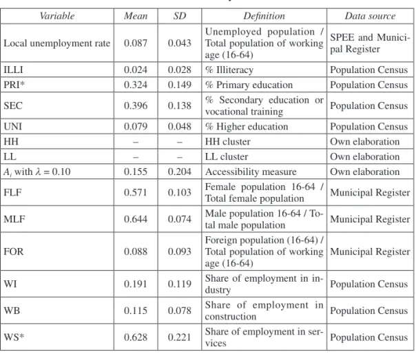
(11) How important is access to employment offices in Spain? An urban and non-urban perspective 129. From a political perspective, insofar as the relation between unemployment rates and accessibility to employment offices remains negative, investments in accessibility bettering will be regarded as meaningful. Joassart-Marcelli and Giordano (2006) point out that One-Stops are well positioned to serve the unemployed and that access to them does help to reduce local unemployment rates. In our study, it should be taken into account that the accessibility variable covers the idea that, whenever a job-seeker finds work, the unemployment rate in their municipality of residence is reduced, accessibility levels (wj) grow in municipalities within the same regional labor office and, consequently, the performance of the employment services improves. When we refer to employment services, we mean not only job-seeking mediation but also career counseling, which allows the identification and development of each individual’s talent (2008 SPEE Annual Report). Regional unemployment differentials have been analyzed theoretically and empirically. Elhorst (2003) has reviewed the papers on regional and labor economics published since 1985. He asserts that «Whichever model is used, [...] they all result in the same reduced form equation of the regional unemployment rate». In this equation, labor supply, labor demand and wage-setting factors are usually used as explanatory variables, but in this case, as we work with a high level of disaggregation, the available information is limited. Consequently, the model in this paper includes as explanatory variables the rates of foreign population and males and females of working-age, the educational attainment of the population, industries’ employment shares and two dummy variables, one for municipalities within high-high (HH) clusters of unemployed and the other for municipalities within low-low (LL) ones 3. The local accessibility level to placement offices is also included. All the variable related information is in Table 2. The basic specification is:. ( ). ( ). log ui = η log Ai + β X i + ei. (2). where ui is the unemployment rate of each municipality, Ai is the accessibility measure and the X matrix collects the explanatory variables described above. Since there are no data on the economically active population at municipal level, local unemployment rates have been calculated by dividing the number of unemployed workers registered at PES offices by the number of people of working age (i.e., population aged 16-64) on the 2009 municipal register. Alonso-Villar and Río (2008) and Alonso-Villar et al. (2009) also rely on this definition to obtain unemployment rates at municipal level. When spatial data are analyzed two different types of spatial effects appear: spatial dependence and spatial heterogeneity. Spatial dependence and spatial heterogeneity are really difficult to disentangle between them. In this idea, Florax et al. (2002) asserted that: «spatial heterogeneity and spatial dependence usually concur as meaningful interpretations of a spatial process because the uniqueness or heterogeneity of 3 These clusters are identified by means of local indicator of spatial association (LISA, Anselin,1995) in Suárez (2011).. 08-SUAREZ.indd 129. 24/2/12 09:26:02.

(12) 130. Suárez, P., Mayor, M. and Cueto, B.. Table 2. Variable. Mean. Summary statistics. SD. Local unemployment rate. 0.087. 0.043. ILLI PRI*. 0.024 0.324. 0.028 0.149. SEC. 0.396. 0.138. UNI HH LL Ai with l = 0.10. 0.079 – – 0.155. 0.048 – – 0.204. FLF. 0.571. 0.103. MLF. 0.644. 0.074. FOR. 0.088. 0.093. WI. 0.191. 0.119. WB. 0.115. 0.078. WS*. 0.628. 0.221. Definition Unemployed population / Total population of working age (16-64) % Illiteracy % Primary education % Secondary education or vocational training % Higher education HH cluster LL cluster Accessibility measure Female population 16-64 / Total female population Male population 16-64 / Total male population Foreign population (16-64) / Total population of working age (16-64) Share of employment in industry Share of employment in construction Share of employment in services. Data source SPEE and Municipal Register Population Census Population Census Population Census Population Census Own elaboration Own elaboration Own elaboration Municipal Register Municipal Register Municipal Register Population Census Population Census Population Census. * The percentage of population with incomplete primary education and the share of employment in agriculture have been omitted so as to avoid multicollinearity.. an attribute observed for a subset of the data can coincide with spatial proximity and hence autocorrelation for that attribute among the same observations». We focused in discrete spatial heterogeneity where spatial instability of the parameters is linked to the characteristics of each spatial unit (municipalities in this case). In the discrete case, the spatial observations can be grouped in such a way that the variation pertains to different spatial subsamples, where each group can be treated as homogeneous 4. This can be easily modeled by means of spatial regimes. In this method, prior information is needed to define these spatial subsets, and in this study we distinguish three types of municipalities based on the urban/non-urban classification described above. We explore whether this spatial heterogeneity can be given a substantive interpretation in the sense that different spatial regimes apply for the different types of municipalities. 4. This type of models is commonly applied to test the convergence hypothesis (e.g. Ramajo et al.,. 2008).. 08-SUAREZ.indd 130. 24/2/12 09:26:02.

(13) How important is access to employment offices in Spain? An urban and non-urban perspective 131. A specification allowing for these spatial regimes in the equation should be considered:. ( )  log( A ) ( ) =  0  ( )  0.  log ulu   log usu  log unu.  X lu  + 0 0 . 0. lu. 0 X su 0. ( ). log Asu.    βlu X nu  0 0.   ηlu    0  ηsu  +    log Anu  ηnu  0. 0. β su. ( ).  elu    β nu  + esu  enu   . (3). In the previous section we have established theoretically and empirically the existence of spatial dependence in unemployment rates, so the suitability of some kind of spatial model should be considered. Furthermore, symptoms of spatial instability are detected in the next section, so we propose different spatial regimes to incorporate discrete heterogeneity.. 3.2. Empirical model. Firstly, model [2] has been estimated by means of OLS (Table 3). Both local unemployment rates and accessibility measures have been considered in logarithmic form, but it should be stressed that the use of these variables in levels makes no considerable difference. All the control variables are significant (with the exception of MLF and WI) and the estimated coefficients present the expected signs in accordance with previous theoretical and empirical studies. The effect of the accessibility to placement offices is significant and negative, the unemployment rate decreases —ceteris paribus— by 0.062% when accessibility rises by 1% 5. Standard tests have been carried out so as to assess the adequacy of the regression. The Breusch-Pagan test points to heteroskedascity, which in turn is related to the different sizes of the municipalities considered. In any case, since spatial dependences may cause this heteroskedasticity (McMillen, 1992), the result has been interpreted with caution. We may also note that the Kolmogorov-Smirnov test has led us to reject the assumption of normality of the OLS residuals. Another issue is whether the accessibility variable is endogenous. Wooldridge’s score test (1995) has been carried out so as to check the endogeneity of the accessibility variable. This test, whose instruments are geographic (municipality surface) and 5 Suárez (2011) analyze the sensitivity of the estimated accessibility elasticities according to the possible values of the distance decay parameter.. 08-SUAREZ.indd 131. 24/2/12 09:26:02.

(14) 132. Suárez, P., Mayor, M. and Cueto, B.. Table 3. OLS regression of local unemployment rate OLS (White) Intercept. –3.007 (0.073)***. Ai with l = 0.10. –0.062 (0.005)***. FLF MLF. 0.894 (0.111)*** –0.051 (0.137). HH. 0.291 (0.019)***. LL. –0.119 (0.015)***. ILLI. 3.501 (0.205)***. PRI. –0.075 (0.045)*. SEC. –0.266 (0.054)***. UNI. –2.033 (0.122)***. FOR. –0.529 (0.051)***. WB. 0.363 (0.047)***. WI. 0.072 (0.048). WS Breusch-Pagan test. 0.154 (0.039)*** 232.3***. Kolmogorov-Smirnov. 0.246***. R (adj.). 0.278. 2. Log-likelihood AIC. –2,525.216 5,080.432. demographic characteristics, is more appropriate when the residuals show heteroskedasticity. In this case, the endogenous regressors are actually exogenous 6. Hence the OLS estimator is more efficient. Moran’s I is widely used to detect spatial dependences based on OLS residuals. The resulting statistic standard deviation is 41.815***. Here we have used a row-standardized rook contiguity matrix so that w sij = wij / ∑j wij when i ≠ j and w sij = 0 when i = j. Nevertheless, it is necessary to analyze the existence of spatial heterogeneity and disentangle it from spatial autocorrelation. Then, equation [3] is estimated by means of OLS. Again, Moran’s I statistic is highly significant (43.142***) and points to the existence of spatial autocorrelation in the residuals. Once spatial autocorrelation has been detected, we may proceed to incorporate it into the proposed model. In spatial econometrics, spatial autocorrelation is modeled by means of the relation between the dependent variable Y or the error term and its associated spatial lag, Wy for a spa6 Unless an instrumental variables estimator is really needed, OLS should be used instead. In this case, the robust regression statistic is 1.295 with a p-value 0.255.. 08-SUAREZ.indd 132. 24/2/12 09:26:02.

(15) How important is access to employment offices in Spain? An urban and non-urban perspective 133. tially lagged dependent variable (spatial lag model) and We for the spatially lagged error term (spatial error model), respectively. Only a few papers deal with how to specify a spatial econometric model (see Mur and Angulo, 2009). Then the problem is how to best identify the structure of the underlying spatial dependences in a given data set. This paper relies on widely used strategy (specific to general), which is based on the LM (Lagrange Multiplier) test and its robust version for local misspecifications (Anselin et al., 1996). In this classical approach, the LMERR (Lagrange Multiplier for error dependence) and the LMLAG (Lagrange Multiplier for spatially lagged dependent variable) are compared. If the LMERR is lower than the LMLAG, the spatial lag model should be specified. If not, the spatial error model is to be specified. Florax et al. (2003) have developed a hybrid approach based on the robust version of these tests 7. These tests have been computed on OLS residuals of the previously estimated models. We have also considered different criteria to build the spatial weight matrices that allowed us to analyze the sensitivity of the results 8. As regards the structure of the spatial effects, three criteria are usually considered in the creation of a spatial weight matrix: contiguity, k-nearest and distance. Firstly, we define a rook contiguity matrix, where wij = 1 if municipalities i and j share a common edge and wij = 0 otherwise. Secondly, we apply a k-nearest neighbors’ criterion (k = 3, 4 and 5). Then, we obtain a distance-based matrix, where wij = 1 if the distance between i and j is less than d and wij = 0 if i = j or d > dij (d = 20, 30 and 40 km). We report the values of the LM specification tests using the rook contiguity matrix, since for the rest of the matrices, these tests and their robust versions render the same conclusions. Both LMERR and LMLAG reject their respective null hypothesis of absence of spatial autocorrelation. The LMLAG (2,253.791***) is greater than LMERR (1,839.588***) and consequently a spatial lag of the dependent variable is included in the model. The robust version of these statistics confirms the diagnostic: R-LMLAG (414.607***) and R-LMERR (0.404; p-value = 0.525). Consequently, a spatial lag specification has been chosen and, more specifically, one based on both the economic theoretical framework and the results of the specification test. Similarly, LeSage and Pace (2009) assert that spatial lag models have been used in contexts where there is a theoretical motivation for Y to be dependent on neighboring values of Y. Molho (1995) and Patacchini and Zenou (2007) provide theoretical explanation for the spatial correlation between unemployment rates. The stability of the regression coefficients (homogeneity) is commonly assessed by means of the Chow test which is adapted by Anselin (1990) to the case of a crosssectional model with a structure of spatial dependence 9. The overall spatial Chow test strongly rejects the joint null hypothesis of structural stability (333.77***). 7 Mur and Angulo (2009), however, point out that the robust and the classical approaches render identical results. 8 These results bring up one of the unsolved questions in spatial econometrics: the selection of the spatial weight matrix (Fernández et al., 2009). 9 Mur et al. (2009) use a broad notion of spatial heterogeneity and propose several test to detect it.. 08-SUAREZ.indd 133. 24/2/12 09:26:02.

(16) 134. Suárez, P., Mayor, M. and Cueto, B.. Maximum likelihood (ML) is the most conventional estimation method for a standard spatial autoregressive model (SAR) where the error terms are assumed to follow a normal distribution. The Generalized Moment Estimator (GME) for the autoregressive parameter in a spatial model, proposed by Kelejian and Prucha (1999), also allows us to solve the problems previously described. They prove that the GM estimator is consistent without the assumption of normality. More recently, Lin and Lee (2010) have shown the robustness of the GMM estimators under unknown heteroskedasticity —a context in which the MLE is usually inconsistent. Generally speaking, it should be noted that the results are qualitatively similar across the different methods: positive value of the spatial autoregresive parameter and negative value of the accessibility estimated coefficient in the non-urban regime 10. In Table 4 we include the estimation results by means of ML and GMM using as spatial weight matrix a k-nearest neighbor matrix k = 5 11. The estimated spatial coefficient is 0.538 when the model is estimated by ML, whereas this value is higher (0.769), when the GMM estimation method is used. In both cases, it is highly significant. A possible explanation for this smaller value could lie in the non-normality of the error term and the aforementioned heteroskedasticity problem 12. Therefore, GMM results are more reliable. We find that the role of employment offices is especially important in non-urban areas where employment opportunities are limited. The estimated coefficient of the accessibility is negative and significant but it is constrained to –0.0314 (ML) or –0.0176 (GMM). In other words, access to employment offices is more likely to be associated with reductions in local unemployment rates in non-urban areas. In terms of policy welfare, this implies that it is very important for employment offices to locate to in non-urban areas with high needs for employment services in order to bridge the gap between unemployed workers and employers where job opportunities are unclear. All coefficients of the control variables —except SEC and WS— are statistically significant in the GMM model (non-urban regime). The percentage of university graduates is significant and negative, whereas those of illiterates and also primary education graduates are significant and positive. As expected, the coefficient of primary education graduates is lower than that of illiterates. With respect to the two other considered regimes (small and large urban) the accessibility variable is not significant. This result is not surprising, and is explained by two reasons. On the one hand, the majority of the urban employment offices have congestion problems so its effect on local unemployment rates may be limited. On 10 The results obtained by means of 2SLS (available from the authors upon request) and GMM methods are quantitative the same. 11 The spatial weight matrices defined in section 3 have also considered to analyze the sensitivity of the results. In all the cases, the spatial lag model is pointed out as the more suitable specification. 12 Lin and Lee (2010) show that the ML estimator is generally inconsistent with unknown heteroskedasticity if the SAR model were estimated as if the disturbances were i.i.d.. 08-SUAREZ.indd 134. 24/2/12 09:26:02.

(17) How important is access to employment offices in Spain? An urban and non-urban perspective 135. other hand, if employment opportunities are higher the role of employment offices could be diminishes. Finally, the residuals of the spatial lag model have been analyzed to check whether the spatial autocorrelation had been fully removed. The result of the LM test is significant to reject the null hypothesis of no spatial correlation in the residual errors. However, as we explained above, the heteroskedasticity problem points to the specification of a model in which such unknown heteroskedasticity in the error term may be controlled. Recently, Kelejian and Prucha (2010) and Arraiz et al. (2010) have extended the GMM approach to a spatial autoregressive disturbance process with heteroskedasti city innovations. The general form is: log(u) = ρW1 log(u) + η log( A) + X β + e. (4). e = θW2e + ε ;. (5). and. In this case, heteroskedasticity of unknown form is permitted with E(ei) = 0 and E(e 2i ). The last column in Table 4 shows the estimation results of this model (GMM-HET). Again, we have obtained a strong spatial dependence between local unemployment rates with a significant spatial effect. The estimated coefficient of the accessibility measure is negative and statistically significant in non-urban areas (–0.0122) and non-significant in small and large urban areas. With respect to the control variables there are some changes: WS is significant and PRI and MLF are not. However, the interpretation of the parameters is more complicated in models containing the spatial lag of the dependent variable. Any change in the dependent variable for a single area may affect the dependent variable in all the other areas. Thus, a change in one explanatory variable in the municipality i will not only exert a direct effect on its own unemployment rate, but also an indirect effect on the unemployment rates of other municipalities. Consequently, the interpretation of the effects on dependent variable Y of a unit change in an exogenous variable Xj, the derivative ∂Y/∂Xj, is not simply equal to the regression coefficient since it also takes account of the spatial interdependencies and simultaneous feedback embodied in the model. As the partial derivative impacts take the form of a matrix (I – rW)–1 Ibj, LeSage y Pace (2009) propose new scalar summary measures to collect all these interactions between municipalities so that we may reach a correct interpretation of the spatial models and distinguish between the direct and the indirect impact. Then, the direct impact shows the average response of the dependent variable to independent variables, including feedback influences that arise from impacts passing through neigh-. 08-SUAREZ.indd 135. 24/2/12 09:26:03.

(18) 08-SUAREZ.indd 136. ML. –0.0314*** –0.0018. 1.8744***. Access. ILLI. –1.6118*** –1.1530**. –0.3400*** –0.5655*** –0.0669. FOR. 0.1323***. 0.2630***. 0.0793**. WI. WB. WS. 0.4724 6,292. R2. N. AIC. 3,021.100. –1,472.531. 0.2804***. KolmogorovSmirnov. Log-likelihood. 278.885***. —. 0.5386. –0.1297. 0.3721**. 0.3298**. Spatial BreuschPagan. Lambda. Rho. 0.1738. MLF. 2.1996**. 0.3806*** –0.7780. FLF. Small. GMM. 0.0279. 0.0025. 0.0805** 0.0258. –0.6145. 1.1412*** –0.6780. –0.0176***. –0.9384*** –0.8425**. Non-urban. –0.2598**. 0.2261. –0.3514**. 1.7915***. –0.4286. 0.0487. 0.2165***. 0.1421***. 0.2603**. 0.1645**. —. —. 6,292. 0.5327. 0.2383***. 282.535***. –. 0.7698***. –0.1618. 0.3976**. 0.2594. 2.0410**. –2.2189**. –0.2232*** –0.3579**. –1.0679*** –1.1364*** –0.9977*. –0.0416. –0.0064. UNI. 0.1199. –0.1953. 0.0345. –0.0811**. SEC. 4.5228***. 0.0124. –0.1548. Large. PRI. 0.7592. –1.5588*** –0.2770. Small. Non-urban. Small. GMM-HET. –0.2645**. 0.2335. –0.2713. 2.0918***. –1.0376**. 0.0188. –0.7868**. 0.1735. 0.1200. 3.1753***. 0.0172. 0.3841**. 0.1941. 0.2463. 1.5470***. –0.7421**. 0.0099. –0.6275***. 0.0449. –0.0577. 2.2868***. 0.0143. –0.0480. Large. 0.2460**. —. —. 6,292. 0.5242. 0.2791***. 256.921***. –0.6266***. 0.8310***. –0.2134**. 0.1292. 0.3672*** –0.1256**. 1.6906***. –1.1967**. 0.0891*** –0.0144. 0.1816***. 0.1155***. 0.1119. 1.1597**. –0.1564*** –0.3577***. –0.8588*** –0.2100. 0.0035. 0.0479. 0.9497***. –0.0122*** –0.0004. –1.1355*** –0.6940*** –0.2335. Large. Estimation Results for the Spatial Regimes Spatial Lag Model. Intercept. Non-urban. Table 4.. 136 Suárez, P., Mayor, M. and Cueto, B.. 24/2/12 09:26:03.

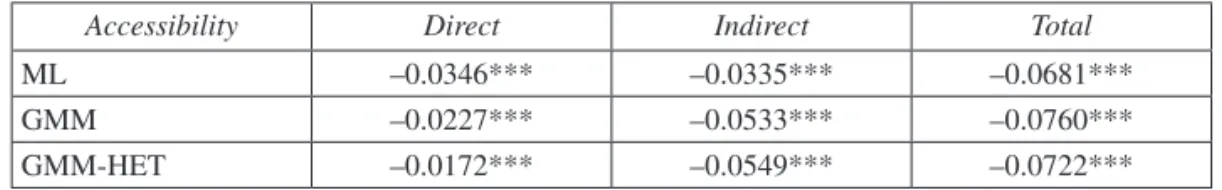
(19) How important is access to employment offices in Spain? An urban and non-urban perspective 137. bours and back to the municipality itself 13. The indirect impact tackles the effect that any change in a region has on others, and how changes in all regions affect a region. These effects can be summarized by their mean. The average total effect of a unit change in Xj is N. N −1 ∑ ir. ∂Yi = N −1i′ I − ρW ∂X rj. (. ). −1. Iβj i. (6). and this effect can be partitioned into a direct and an indirect component in all cells of Xj. The average direct impact is given by the mean of the main diagonal of the matrix, hence N. N −1 ∑ r. ∂Yr = N −1 trace  I − ρW  ∂X r j. (. ). −1. Iβ j  . (7). The difference between the total effect and the direct effect is the average indirect effect of a variable, that is, it is equal to the mean of the off-diagonal cells of the matrix (I – rW)–1 Ibj ∂Yr = I − ρW ∂ r ≠ s Xsj N. N −1 ∑. Table 5.. (. ). −1. (. I β j i − N −1 trace  I − ρW . ). −1. Iβ j  . (8). Direct, indirect and total impact estimations: non-urban municipalities. Accessibility. Direct. Indirect. Total. ML. –0.0346***. –0.0335***. –0.0681***. GMM. –0.0227***. –0.0533***. –0.0760***. GMM-HET. –0.0172***. –0.0549***. –0.0722***. The accessibility to placement offices has a slightly higher (and significant) direct effect than the coefficient estimate. This difference is caused by impacts passing through neighboring regions and back to the region itself. Consequently, a positive feedback effect is obtained. Even more interesting is the estimation result of the indirect impact, which is significant and three times higher than the coefficient estimate in the GMM model, showing a positive influence of the accessibility to placement offices across the spatial dependences between municipalities. The total impacts are –0.0760 for GMM and –0.0722 for GMM-HET. This means that if accessibility increases by 1%, the unemployment rate decreases —ceteris paribus— by 0.0760%/ 0.0722%, respectively. 13 The main diagonal of higher order spatial weight matrices is non-zero, which allows us to collect these feedback effects.. 08-SUAREZ.indd 137. 24/2/12 09:26:03.

(20) 138. Suárez, P., Mayor, M. and Cueto, B.. Thus, the presence of heteroskedasticity has no main effect on the coefficient estimates of this empirical model when GMM and GMM-HET methods are compared. All these approaches have been applied to the study of local unemployment rates and we have found that the accessibility measure helps to reduce them.. 4.. Conclusions and policy recommendations. In this paper we investigate whether a specific strategy of allocating employment offices and different levels of accessibility to the employment offices can contribute to a reduction of local unemployment rate on the municipality level. Given the limited knowledge about the role of employment offices in Spain, our analysis contributes to this field of research in several ways. Firstly, from the methodological point of view, the modeling techniques applied in this paper highlight the importance of accounting for spatial dependence and spatial heterogeneity in the analysis of the role of organizations like the Public Employment Services. Using ML and GMM methods, we have shown a strong spatial correlation between unemployment rates, i.e. that neighborhood influences are very important in labor markets. This view is consistent with other empirical studies such as Molho (1995) and Patacchini and Zenou (2007) and, therefore, the spatial perspective cannot be ignored in the analysis of the Spanish labor market. Secondly, we have obtained that there are spatial differences across the employment offices in Spain, even though employment offices are located around urban municipalities. We find an inverse relationship between access to employment offices and local unemployment rates in non-urban municipalities. In addition to that, when we compute the direct and indirect impacts of the accessibility measure on unemployment rates in non-urban areas, the indirect impact is shown to be higher than the estimated coefficient. This, in turn, shows a positive influence on the reduction of unemployment rates across the spatial interactions bet ween municipalities. In contrast, in urban municipalities this relationship is not clear. It may be due to the congestion problem and the high level of employment opportunities in urban municipalities. The results suggest that policy makers should strive to improve the accessibility to placement offices, especially in the non-urban municipalities.. References Alonso-Villar O., and Río, C. del (2008): «Geographical Concentration of Unemployment: A Male-Female Comparison in Spain», Regional Studies, 42: 401-412. Alonso-Villar O.; Río, C. del, and Toharia, L. (2009): «Un análisis espacial del desempleo por municipios», Revista de Economía Aplicada, 49: 47-80.. 08-SUAREZ.indd 138. 24/2/12 09:26:03.

(21) How important is access to employment offices in Spain? An urban and non-urban perspective 139. Althin R., and Behrenz, L. (2004): «An efficiency analysis of Swedish Employment Offices», International Review of Applied Economics, 18: 471-482. Anselin, L. (1990): «Spatial dependence and spatial structural instability in applied regression analysis», Journal of Regional Science, 30: 185-207. — (1995): «Local indicators of spatial association -LISA», Geographical Analysis, 27: 93-115. Anselin, L., Bera, A., Florax, R., and Yoon, M. (1996): «Simple diagnostic tests for spatial dependence», Regional Science and Urban Economics, 26: 77-104. Arraiz, I.; Drukker, D. M.; Kelejian, H. H., and Prucha, I. R. (2010): «A spatial Cliff-Ord-type model with heteroskedastic innovations: small and large sample results», Journal of Regional Science, 50: 592-614. Assunçao, R. M., and Reis, E. A. (1999): «A new proposal to adjust Moran’s I for population density», Statistics in medicine, 18: 2147-2162. Bröcker, J. (1989): «How to eliminate certain defects of the potential formula», Environment and Planning A, 21: 817-830. CES (2009): Memoria sobre la situación socioeconómica y laboral en España, Consejo Económico y Social. Cliff, A., and Ord, J. K. (1981): Spatial processes: models and applications, Pion, London. Détang-Dessendre, C., and Gaigné, C. (2009): «Unemployment duration, city size, and the tightness of the labor market», Regional Science and Urban Economics, 39: 266-276 Elhorst, J. P. (2003): «The mystery of regional unemployment differentials: theoretical and empirical explanations», Journal of Economic Surveys, 17: 709-748. Fernández, E.; Mayor, M., and Rodríguez, J. (2009): «Estimating autorregresive spatial models by GME-GCE techniques», International Regional Science Review, vol. 32, pp. 148-172. Fertig, M.; Schmidt, C. M., and Schneider, H. (2006): «Active labor market policy in Germany -Is there a successful policy strategy», Regional Science and Urban Economics, 36: 399-430. Florax, R. J. G. M.; Folmer, H., and Rey, S. (2003): «Specification searches in spatial econometrics: the relevance of Hendry’s methodology», Regional Science and Urban Econo mics, 33: 557-579. Florax, R. J. G. M.; Voortman, R. L., and Brouwer, J. (2002): «Spatial dimensions of precision agriculture: a spatial econometric analysis of millet yield on Sahelian coversands», Agricultural Economics, 27: 425-443. Frost, M. E., and Spence, N. A. (1995): «The rediscovery of accessibility and economic potencial: the critical issue of self-potential», Environment and Planning A, 27: 1833-1848. Fujita, M.; Krugman, P., and Venables, A. J. (1999): The Spatial Economy. Cities, regions and international trade. MIT Press, Cambridge, MA. Geurs, K. T., and van Wee, B. (2004): «Accessibility evaluation of land-use and transport stra tegies: review and research directions», Journal of Transport Geography, 12: 127-140. Gutiérrez, J. (2001): «Location, economic potential and daily accessibility: an analysis of the accessibility impact of the high-speed line Madrid-Barcelona-French border», Journal of Transport Geography, 9: 229-242. Gutiérrez-i-Puigarnau, E., and van Ommeren, J. N. (2010): «Labor supply and commuting», Journal of Urban Economics, 68: 82-89. Hagen, T. (2003): «Three approaches to the evaluation of active labour market policy in East Germany using regional data», ZEW Discussion Paper, 03-27, ZEW-Mannheim. Holl, A. (2007): «Twenty years of accessibility improvements. The case of the Spanish motorway building programme», Journal of Transport Geography, 15: 286-297. Ihlanfeldt, K. R. (1997): «Information on the spatial distribution of job opportunities within metropolitan areas», Journal of Urban Economics, 41: 218-242. Joassart-Marcelli, P., and Giordano, A. (2006): «Does local access to employment services reduce unemployment? A GYS analysis of One-Stop Career Centers», Policy Sciences, 39: 335-359.. 08-SUAREZ.indd 139. 24/2/12 09:26:03.

(22) 140. Suárez, P., Mayor, M. and Cueto, B.. Kelejian, H. H., and Prucha, I. R. (1999): «A generalized moments estimator for the autoregressive parameter in a spatial model», International Economic Review, 40: 509-533 — (2010): «Specification and estimation of spatial autoregressive models with autoregressive and heteroskedastic disturbances», Journal of Econometrics, 157: 53-67 Krugman, P. (1991): «Increasing returns and economic geography». Journal of Political Eco nomy, 99: 483-499. LeSage, J., and Pace, R. K. (2009): Introduction to Spatial Econometrics, CRC Press. Lin, X., and Lee, L. F. (2010): «GMM estimation of spatial autoregressive models with unknown heteroskedasticity», Journal of Econometrics, 157: 34-52. López-Bazo, E.; del Barrio, T., and Artis, M. (2002): «The regional distribution of Spanish unemployment: A spatial analysis», Papers in Regional Science, 81: 365-389. McMillen, D. P. (1992): «Probit with spatial autocorrelation», Journal of Regional Science, 32: 335-48. Molho, I. (1995): «Spatial autocorrelation in British unemployment», Journal of Regional Science, 35: 641-658. Mur, J., and Angulo, A. (2009): «Model selection strategies in a spatial setting: some additional results», Regional Science and Urban Economics, 39: 200-213. Mur, J.; López, F., and Angulo, A. (2009): «Testing the hypothesis of stability in spatial econometric models», Papers in Regional Science, 88: 409-444. Overman, H. G., and Puga, D. (2002): «Unemployment clusters a cross euro’s regions and countries», Economic Policy, 17:115-148. Patacchini, E., and Zenou, Y. (2007): «Spatial dependence in local unemployment rates», Journal of Economic Geography, 7: 169-191. Ramajo, J.; Márquez, M. A., Hewings, G. J. D., and Salinas, M. M. (2008): «Spatial heterogeneity and interregional spillovers in the European Union: Do cohesion policies encourage convergence across regions?», European Economic Review, 22: 551-567. Sheldon, G. M. (2003): «The efficiency of public employment services: a nonparametric matching function analysis for Switzerland», Journal of Productivity Analysis, 20: 49-70. SPEE (2008): Memoria del Servicio Público de Empleo Estatal 2008. Suárez, P. (2011): «El Servicio Público de Empleo en España: ensayos desde una perspectiva regional», PH. D. Tesis, Universidad de Oviedo, Spain. Talen, E., and Anselin, L. (1998): «Assessing spatial equity: an evaluation of measures of accessibility to public playgrounds», Environment and Planning A, 30: 595-613. Tsou, K. W.; Hung, Y. T., and Chang, Y. L. (2005): «An accessibility-based integrated measure of relative spatial equity in urban public facilities», Cities, 22: 424-435. Van Wee, B.; Hagoort, M., and Annema, J. A. (2001): «Accessibility measures with competition», Journal of Transport Geography, 9: 199-208. Wooldridge, J. M. (1995): «Score diagnostics for linear models estimated by two stage least squares», en: Maddala, G. S.; Phillips, P. C. B., and Srinivasan, T. N. (eds.), Advances in Econometrics and Quantitative Economics: Essays in Honor of Professor C. R. Rao, Blackwell, Oxford. Zwakhals, L.; Ritsema van Eck, J.; Jong, T., and Floor, H. (1998): «Flowmap for windows 6.0 hands-on», Accessibility analysis and gravity models, Faculty of Geographical Sciences, Utrecht University.. 08-SUAREZ.indd 140. 24/2/12 09:26:03.

(23)