communications
Georgina Stegmayer1 and Omar Chiotti2
1 C.I.D.I.S.I., Universidad Tecnol´ogica Nacional, Lavaise 610, 3000 Santa Fe,
Argentina. e-mail:gstegmay@frsf.utn.edu.ar
2 INGAR-CONICET, Avellaneda 3654, 3000 Santa Fe, Argentina. e-mail:
chiotti@ceride.gov.ar
Abstract. This paper presents a time-delayed neural network (TDNN) model that has the capability of learning and predicting the dynamic behavior of nonlinear elements that compose a wireless communication system. This model could help speeding up system deployment by reducing modeling time. This pa-per presents results of effective application of the TDNN model to an amplifier, part of a wireless transmitter.
1 Introduction
In new generation wireless communications - i.e. third generation (3G) stan-dards such as WCDMA (Wideband Code Multiple Division Access) and UMTS (Universal Mobile Telecommunications System) towards which most of the cur-rent cellular networks will migrate - system component modeling has become a critical task inside the system design cycle, due to modern digital modulation schemes [1].
New standards may introduce changes in the behavior of the devices that are part of the system (e.g. mobile phones and their internal components) mainly due to the modulation schemes they use, generating nonlinearities in the be-havior and memory effects (when an output signal depends on past values of an input signal). Memory effects in the time-domain cause the output of an elec-tronic device to deviate from a linear output when the signal changes, resulting in the deterioration of the whole system performance since the device begins behaving nonlinearly. In this work we are interested in modeling the nonlinear behavior that an amplifier can have inside a wireless transmission.
the data signal. The signal has to reach an antenna from the cellular phone with enough strength to guarantee the communication. But the signal suffers from attenuation and needs amplification before that. Therefore, the final element of the chain is a power amplifier (PA) which amplifies the signal before it travels to the nearer antenna and to the receiver side of the communications chain.
Fig. 1.Simplified block diagram of a digital wireless transmitter.
An amplifier works by increasing the magnitude of an applied signal. Am-plifiers can be divided into two big groups: linear amAm-plifiers, which produce an output signal directly proportional to the input signal, and power amplifiers which have the same function as the first ones, but their objective is to obtain maximum output power. A PA can work in different ”classes”: in Class A if it arrives at the limit of the linearity; and class B when it works in nonlinear regime. Moreover, in wireless communications, the transmitter itself introduces nonlinearities when operating near maximum output power [2].
Nonlinear behavior modeling has been object of increasing interest in the last years [3][4] since classical techniques that were traditionally applied for modeling are not suitable anymore. That is why new techniques and methodologies have been recently proposed, as for example neural network (NN) based modeling applied to PA modeling[5].
Neural networks, as a measurement-based technique, may provide a compu-tationally efficient way to relate inputs and outputs, without the computational complexity of full circuit simulation or physics level knowledge [6], therefore significantly speeding up the analysis process. No knowledge of the internal structure is required and the modeling information is completely included in the device external response.
Although the NN approach has been largely exploited for static simulation, their application to dynamic systems modeling is a rather new research field. In this paper we present a new NN model for modeling nonlinear elements that belong ro a communications chain, using a network which takes into account device nonlinearity and memory effects. In particular, this paper presents the results of the proposed model to nonlinear PA modeling.
2 Neural network-based modeling
Neural network-based models are nowadays seen as a potential alternative for modeling electronics elements having medium-to-strong memory effects along with high-order nonlinearity. NNs are preferred over traditional methods (i.e. equivalent-circuit, empirical models) because of their speed in implementation and accuracy. A NN model can be used during the stage of system design for a rapid evaluation of its performance and main characteristics. The model can be directly trained with measurements extracted from the real system, speeding up the design cycle. NN models can be more detailed and rapid than traditional equivalent-circuit models, more exact and flexible than empirical models, and easier to develop when a new technology is introduced. By profiting from their potential to learn a device behavior based on simulated or measured records of its input and output signals, they were used in nonlinear modeling and design of many microwave circuits and systems [7].
The increasing number of electronic devices models proposed using NNs that have appeared in the last years [8][13][10] shows their importance and interest. Many topologies of NNs are reported in the literature for modeling different types of circuits and systems, with different kinds of linear and nonlinear be-havior [11]. However, until very recently, NNs for modeling were applied almost exclusively to instantaneous behavior of the input variables alone. Although this approach has been largely exploited for static simulation, their application to dynamic system is a rather new research field. Recently have appeared NN-based models taking into account the dynamic phenomena in RF microwave devices [12].
For representation of a system which has a nonlinear behavior and is dy-namic, intending by dynamic not only that the device characteristic varies over time but also that it depends on past values of its controlling input variables, not any NN topology can be used. A neural model which includes time-dependence into the network architecture is the time-delayed neural network (TDNN), a special type of the well-known multilayer-perceptron (MLP). TDNNs have been successfully applied for solving the temporal processing problems in speech recognition, system identification, control and signal modeling and processing [13]. They are suited for dynamic systems representation because the contin-uous time system derivatives are approximated inside the model by discrete time-delays of the model variables.
Fig. 2. Time-Delayed neural network (TDNN) model and its corresponding input data.
In this paper we propose the application of a TDNN model for modeling nonlinear and dynamic behavior of devices or elements, parts of a communica-tion system. The model proposed is explained in detail in the next Seccommunica-tion.
3 TDNN model
The proposed model has the classical three layers topology for universal approx-imation in a MLP: the input variable and its delayed samples, the nonlinear hidden layer and a linear combination of the hidden neurons outputs at the output neuron. The architecture of the TDNN is shown in figure 3.
Fig. 3. Time-Delayed neural network (TDNN) to model a communications chain component.
[image:4.612.200.412.363.530.2]In the hidden layer, the numberhof hidden neurons varies between 1 and H. The hidden units have a nonlinear activation function. In general, the hy-perbolic tangent (tanh) will be used because this function is usually chosen in the electronics field for nonlinear behavior. In our model we have used H = 10, but if necessary, the number of neurons in the hidden layer can be changed to improve the network accuracy. The hidden neurons receive the sum of the weighted inputs plus a corresponding bias value for each neuronbh. All the neu-rons have bias values. This fact gives more degrees of freedom to the learning algorithm and therefore more parameters can be optimized, apart from weights, to better represent a nonlinear system.
The weights between layers are described with the usual perceptron no-tation, where the sub-indexes indicate the origin and the destination of the connection weight, e.g. wj,i means that the weight w relates the destination neuron j with the origin neuron i. However, a modification in the notation was introduced, adding a super-index to the weights, to more easily identify to which layer they belong. Therefore,w1
means that the weightwbelongs to the connection between the inputs and the first hidden layer, and w2
means that the weight wbelongs to the connection between the first hidden layer and the second one (in our particular case, the second hidden layer happens to be the output layer). In this second group of connections weights, the sub-index which indicates the destination neuron has been eliminated because there is only one possible destination neuron (the output).
This unique output neuron has a linear activation function which acts as a normalization neuron (this is usual choice in MLP models). Therefore, the output of the proposed TDNN model is calculated as the sum of the weighted outputs of the hidden neurons plus the corresponding output neuron bias (b0),
yielding equation 1.
yN N(t) =b0+
"H
X
h=1
w2
htanh bh+ N
X
i=0
w1
h,i+1x(t−i)
!#
(1)
Network initialization is an important issue for training the TDNN with the back-propagation algorithm, in particular in what respects speed of execution. In this work the initial weights and biases of the model are calculated using the Nguyen-Widrow initial conditions [14] which allow reducing training time, instead of a purely random initialization.
Once the TDNN model has been defined, it is trained with time-domain measurements of the element output variable under study (yout(t)), which is expressed in terms of its discrete samples. To improve network accuracy and speed up learning, the inputs are normalized to the domain of the hidden neu-rons nonlinear activation functions (i.e for the hyperbolic tangent tanh, the interval is [−1; +1]). The formula used for normalization is shown in equation 2.
xnorm= 2 (x−min{x})
During training, network parameters are optimized using a backpropaga-tion algorithm such as the Levenberg-Marquardt [15], chosen due to its good performance and speed in execution. To evaluate the TDNN learning accuracy, the mean square error (mse) is calculated at each iterationkof the algorithm, using equation 3, where P is the number of input/output pairs in the training set, yout is the output target andyN N is the NN output.
mse= 1 P
P
X
k=1
E(k)2
= 1 P
P
X
k=1
(yout(k)−yN N(k))2 (3)
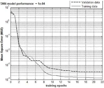
The good generality property of a NN models says that it must perform well on a new dataset distinct from the one used for training. Even a excessive number of epochs or iterations on the learning phase could make performance to decrease, causing the over-fitting phenomena. That is why, to avoid it, the total amount of data available from measurements is divided into training and validation subsets, all equally spaced. We have used the ”early-stopping” tech-nique [16], where if there is a succession of training epoch in which accuracy improves only for the training data and not for the validation data, over-fitting has occurred and the learning is terminated. The obtained results are shown in the next section.
4 Measurements and validation results
For training the neural model, a dedicated test-set for accurate PA charac-terization has been used. It provides static and pulsed DC characcharac-terization, scattering parameter measurements, real-time load/source-pull at fundamen-tal and harmonic frequencies, and gate and drain time-domain RF waveforms. The measurements are carried out with a Microwave Transition Analyzer and a large-signal Vector Network Analyzer.
Complete characterization was performed for different input power levels and different classes of operation at 1 GHz on a 2 ns window, as shows figure 4. Class A is biased at 50% IDSS, and class B withIDS= 0. A 1 mm total gate periphery GaN HEMT based on SiC with IDSS = 700 mA, has been measured at 1 GHz. The power sweep ranged from -21 to +27 dBm. Only the first 4 harmonics are taken into account.
Fig. 4. Time-domain waveforms at 1 GHz at increasing power for class A (top), and B (bottom) at 50 Ohm load used for training.
used for model validation. In principle, however, this method does not need full load-pull characterization, but only to map gate and drain nonlinear models for different generic tuned-loads, in order to concern the widest region in the I-V characteristic. Input data vectors of VGS and VDS for each load and power level have been first copied and delayed as many times, to represent the network inputs, as necessary to account for memory, and then joined together to train the TDNN model with all the working classes, the selected load terminations and the power levels, simultaneously. This is shown in figure 5.
Fig. 5.TDNN model training data organization.
[image:7.612.239.378.409.552.2]modelled data, in fact the relative mean square error is lower than 1e-04 (figure 6).
Fig. 6.TDNN model performance.
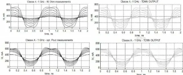
[image:8.612.147.467.412.544.2]Figure 7 reports the output PA time-domain waveforms at increasing output power at 50 Ohm load: the upper plots are relative to a class A condition, while the bottom ones refer to class B operations. The left figures report the measure-ments, while the right ones show the TDNN simulation result. Figure 8 shows the comparison between the training (left) and validation (right) measurement data used for class A operation and the TDNN model response.
Fig. 7. Time-domain waveforms at 1 GHz at increasing power for class A (top), and B (bottom). Measurements (left), TDNN output (right). The pointed arrow waveform refers to a validation data subset.
model predictive capabilities. The model is also capable of recognizing the class in which the device is working and in consequence give a reasonable output response.
Fig. 8.Time domain waveforms at 1 GHz at increasing power for class A at 50 Ohm (used for training), and optimum Pout (used for validation). Measurements (left), TDNN output (right).
5 Conclusions
In this paper, a model that has the capability of learning and predicting the dynamic behavior of nonlinear PAs, based on a Time-Delayed Neural Network (TDNN), has been proposed. Validation and accuracy of the TDNN model in the time-domain showed good agreements between the TDNN model output data and measurements.
The TDNN model can be trained with input/output device measurements or simulations, and a very good accuracy can be obtained in the device char-acterization easily and rapidly. These properties make this kind of models spe-cially suitable for new wireless communications components modeling, which are mostly nonlinear and require speed, accuracy and simplicity when design-ing and builddesign-ing the model.
6 Acknowledgement
References
1. Evci C, Barth U, Sehier P, Sigle R. (2003) The path to beyond 3G systems: strategic and technological challenges. In: Proc. 4th
Int. Conf. on 3G Mobile Communication Technologies, pp. 299-303
2. Elwan H, Alzaher H, Ismail M (2001) New generation of global wireless compat-ibility. IEEE Circuits and Devices Magazine 17: 7-19
3. Ahmed A, Abdalla MO, Mengistu ES, Kompa G. (2004) Power Amplifier Mod-eling Using Memory Polynomial with Non-uniform Delay Taps. In: Proc. IEEE 34th
European Microwave Conf., pp. 1457-1460
4. Ku H, Kenney JS (2003) Behavioral Modeling of Nonlinear RF Power Ampli-fiers considering memory effects. IEEE Trans. Microwave Theory Tech. 51: 2495-2504 5. Root D, Wood J (2005) Fundamentals of Nonlinear Behavioral Modeling for RF
and Microwave design. Artech House, Boston
6. Zhang QJ, Gupta KC, Devabhaktuni VK (2003) Artificial Neural Networks for RF and Microwave Design - From Theory to practice. IEEE Trans. Microwave Theory Tech. 51: 1339-1350
7. Zhang QJ, Gupta KC (2000) Neural Networks for RF and Microwave Design. Artech House, Boston
8. Schreurs D, Verspecht J, Vandamme E, Vellas N, Gaquiere C, Germain M, Borghs G (2003) ANN model for AlGaN/GaN HEMTs constructed from near-optimal-load large-signal measurements. IEEE Trans. Microwave Theory Tech. 51: 447-450
9. Liu T, Boumaiza S, Ghannouchi FM (2004) Dynamic Behavioral Modeling of 3G Power Amplifiers Using Real-Valued Time-Delay Neural Networks. IEEE Trans. Microwave Theory Tech. 52: 1025-1033
10. Ahmed A, Srinidhi ER, Kompa G (2005) Efficient PA modelling using Neural Network and Measurement setup for memory effect characterization in the power device. In: Proc. IEEE MTT-S International Microwave Symposium, pp. 1871-1874
11. Alabadelah A, Fernandez T, Mediavilla A, Nauwelaers B, Santarelli A, Schreurs D, Taz´on A, Traverso PA (2004) Nonlinear Models of Microwave Power Devices and Circuits. In: Proc. 12th
GAAS Symposium, pp. 191-194
12. Xu J, Yagoub MCE, Ding R, Zhang QJ (2002) Neural-based dynamic modeling of nonlinear microwave circuits. IEEE MTT-S Int. Microwave Symp. Dig. 1: 1101-1104
13. Liu T, Boumaiza S, Ghannouchi FM (2004) Dynamic Behavioral Modeling of 3G Power Amplifiers using real-valued Time-Delay Neural Networks. IEEE Trans. Microwave Theory Tech. 52: 1025-1033
14. Nguyen D, Widrow B (1990) Improving the learning speed of 2-layer neural networks by choosing initial values of the adaptive weights. In: Proc. IEEE Int. Joint Conf. Neural Networks, vol. 3, pp. 21-26
15. Marquardt DW (1963) An algorithm for least-squares estimation of non-linear parameters. Journal of the Society for Industrial and Applied Mathematics 11: 431-441