An adaptive finite-state automata application to the problem of reducing the number of states in approximate string matching

An Adaptive Finite-State Automata Application to the

problem of Reducing the Number of States in Approximate

String Matching

Ricardo Luis de Azevedo da Rocha1

, Jo˜ao Jos´e Neto1

1

Laborat´orio de Linguagens e T´ecnicas Adaptativas – Escola Polit´ecnica – USP Av. Professor Luciano Gualberto, Trav. 3 N. 158

CEP 05508-900 S˜ao Paulo – SP – Brasil

[email protected],[email protected]

Abstract

This paper presents an alternative way to use finite-state automata in order to deal with approximate string matching. By exploring some adaptive features that enable any finite-state automaton model to change configuration during computational steps, dynamically deleting or creating new transitions, we can actually control the behavior and the topology of the automaton. We use these features for an application to approximate string matching trying to reduce the number of states required.

Keywords

adaptive devices, approximate string matching, finite-state automata, complexity, appli-cation

Workshop

1. Introduction

Finite-state automata are a significant part of the theory of computation, and the models built from them are widely used in areas such as protocol specification, hardware design, and so forth. Despite the fact that such models are simple to create, they define the class of regular languages (type3languages) [8].

The use of simpler models to build complex structures is the main goal of some efforts, such as in [6, 11]. Those researches have in common the use of a basic model, and through some features, make them able to perform much more complex actions. Such as, to accept strings from type0languages [6]. The original adaptive automaton is based on a pushdown automaton [6], and the self-modifying automaton is based on the finite automaton.

We will use a simplified version of the adaptive automaton in our proposal, which is based on the finite automaton [7]. This paper addresses an application to the problem of approximate string matching using the adaptive finite automaton model.

The problem of approximate string matching may be directly addressed to finite-state automata. Since the early 1970’s some algorithms have been developed to deal with it, such as the Knuth-Morris-Pratt [1], or Boyer-Moore [2], and Aho-Corasick [3]. All of them are based on finite-state automata principles.

The subsequent effort raised new ways of implementation, and some new kinds of models [10], but the problem remains unchanged:

Given a text stringT =t1t2. . . t_n, a patternP =p1p2. . . p_m, and an integerk,k ≤m≤

n, we are interested in finding all occurrences of a substringX in stringT such that the distanceD(P, X) between the pattern P and X is less than or equal to k. D(P, X)is some given function that quantifies how closeP andX are, e.g. by counting unmatching symbols.

In the literature we find several ways for measuring such distance, e.g. the Ham-ming distance, where it is allowed to replace a character by another one, or the Leven-shtein distance, where it is allowed to delete a character from the pattern or to insert a character into the pattern (the generalized Levenshtein distance allows two characters to be exchanged) [10].

The Hamming distance between two strings P and X, of equal length, may be defined as the number of positions with mismatching symbols in those strings. The Lev-enshtein distance between two stringsP andX, not necessarily of equal length, may be defined as the minimal number of editing operations (insert, delete, and replace) needed to convertP intoX[10, 4]. In this paper we will use the Hamming distance measure.

Some improvements have been achieved in the running time and the actual ‘size’ of the automaton along the process. Some researchers described new ways to implement automata models in order to get better performance on their algorithms. In the next section we will take into account a reduced model of finite automata, as developed in [4].

2. Finite-State Automata for String Matching

A nondeterministic finite-state automaton is a 5-tupleM = (K,Σ, δ, q0, F), whereK is a finite set of states,Σis a finite set of input symbols,δis a state transition function from

K×(Σ∪ {ǫ})to2K_{,q0 ∈Qis the initial state,F ⊆K is the set of final states, [9].}

p1p2p3p4. If we need an approximate string matching, the nondeterministic finite-state automaton should be like the one shown in figure 2.

p1 p2 p3 p4

σ ∈ Σ

Figure 1: Nondeterministic Finite Automaton.

Figure 2 shows an automaton built for Hamming distance ofk = 3, which allows exact matching at the first path, one mismatch at the second path, and so forth. At the end of each path there is a final state, which identifies the number of mismatches found in the string.

p1 p2 p3 p4 σ ∈Σ

p1 p2 p3 p4 p2 p3 p4

p2 p3 p4 p3 p4

p3 p4 p4

Figure 2: Nondeterministic Finite-State Automaton for Approximate String Matching of the String accepted by the automaton in Figure 1.

For the Levenshtein distance a similar automaton is slightly more complex, be-cause it requires two further edit operations on the exact original string.

The research developped by Holub [4] has shown a way to reduce the number of states in such nondeterministic finite-state automaton, created to fit a given distance function (Hamming distance of k = 3). Holub’s automaton is constructed without the need to identify the number of mismatches in the string, so there is only one final state, and each path may be significantly reduced, as shown in Figure 3.

p1 σ ∈Σ

p1 σ p2

p2 σ p3

p3 σ p4

Figure 3: Holub’s Nondeterministic Finite-State Automaton for Approximate String Matching.

added to the automaton in order to achieve a better result on the number of states, by dynamically keeping in the automaton only the strictly required states and transitions.

3. Adaptive Features

The main result shown by Holub in [4] is achieved by including in the automaton only the states strictly needed for handling the condition. By applying this idea and by creating the needed states at the execution time, we may significantly reduce the total number of states in the automaton.

By doing so we may use the guidelines in [5], where we find a formal introduction to adaptive devices, and explore the concept of general rule-driven devices which may be tailor-made just to fit our specific needs. From this point of view, we are able to create an automaton that is able to modify its own configuration according to the particular needs of the problem currently being solved.

Following [5] let us consider the nondeterministic finite automaton in figure 2 as our starting point for the creation of an adaptive finite-state automaton in the following way:M_sm = (M, AM), whereM_sm stands for adaptive finite-state automaton,M repre-sents the original finite state automaton, andAM describes the mechanism that modifies the shape of the configuration of the automaton.

LetAAbe a fixed set of actions (including a specialnull adaptive actiona0

). AM

contains a set of rules that may change the topology of the automaton. LetARbe the set of all possible sets of such rules forMsm. In this case, any particular action ak ∈ AA

maps the current set of rules AR_t ⊆ AR, defining the automaton into some other set of rules ARt+1 ⊆ AR, which will be the next set of rules defining the automaton until

another action takes place.

ak _:AR→AR

The mechanism AM associates each transition ti ∈ δ of the original finite

au-tomaton to a corresponding pair of actionsbap_andaap _∈AA:

AM ⊆AA×N R×AA

This way we define an adaptive rule arp _{associated to a rule (transition) nr}p _of

the finite automaton as a 3-tuple inAM as:

arp = (bap, nrp, aap)

For each of its moves the adaptive automatonMsmapplies the chosen rulearpin

three steps:

• Activation of an adaptive actionbap _{before applying the rulenr}p_, • Application of a rule (transition)nrp_{, and,}

• Execution of an adaptive actionaap_{after the application ofnr}p_.

Transitions of the adaptive finite-automaton are defined this way: when the au-tomaton is in state qp _{and will perform a rule (transition) nr}p _{= (ba}p_{, nr}p_{, aa}p_{) which}

leads to statesp+1

and modifies the set of states and transitions, there is an activation of the adaptive actionbap_{, then the rule (transition) is performed and changes to states}p+1

, and then the adaptive actionaap _{is performed, and we show those actions byq}p _⊢sp+1

.

Proposition 1 The adaptive actions may be placed in order to change an automaton be-fore or after the rule (transition).

Proof: Following [7], and by induction on the adaptive steps. Suppose we want only to apply adaptive actions before the application of a rule (the proof is similar for the other case). We will create an additional step to each adaptive one which has an adaptive action after the application of a rule. We have thatqp _{⊢ s}p+1

, and the transition isarp ₌

(bap_{, nr}p_{, aa}p_{), at stateq}p

Base: arp _{= (ba}p_{, nr}p_{, aa}p_{), makingp= 0we have two cases:}

First supposing we have no adaptive steps, so there is no adaptive action to apply, which meansar0

= (ba0 , nr0

, aa0

) = nr0

, andq0

⊢s0

.

For the second case supposep= 0, and we have at least one adaptive action at step

0, so beginning from the initial step0we haveq0

⊢s1

, andar0

= (ba0 , nr0

, aa0

), so we need to create another adaptive step between the application of the rulenr0

andaa0

), indeed we can apply:

ar0

= (ba0 , xnr0

, ǫ)additional step→ (aa1 , nr1

, ǫ), whereǫstands for an empty action. But then we need another state, a new one created by actionxnr0

, say state x1

. So after changing the adaptive actionba0

to xba0

in order to delete the original transitionq0

⊢s1

withar0

= (ba0 , nr0

, aa0

)and create two others in its place, but keeping the other actions ofba0

: q0

⊢x1

, andx1

⊢s2

, where the transition from

q0

tox1

is described asar0

= (xba0_{, bnr}0_{, ǫ}

), and fromx1

tos2

as(aa1_{, anr}1_{, ǫ}

), where rules bnr0

andanr1

act as the original action nr0

, but with an additional step.

Hyp.: arq _{= (ba}q_{, nr}q_{, aa}q_{), ∀q such as0 ≤ q ≤ pcan be split in two, where there are}

no adaptive actions after the transition of both.

Step: arp+1

= (bap+1 , nrp+1

, aap+1

) As we have the application of the rules in steps, there must have beenpsteps of the formarp _{= (ba}p_{, nr}p_{, aa}p_{), and each of these}

steps fall into the inductive hypothesis. The last step can be split in two just as before (in base case, wherep= 0with1adaptive step):

arp+1

= (xbap+1

, bnrp+1

, ǫ)additional step→ (aap+2

, anrp+2 , ǫ)

♦

Adaptive finite-state automata were designed from classic finite-state automata [8, 9], and may be viewed as a set of finite-state automata grouped together by the possibility of each one be replaced by some other one by changing the topology of the currently used one.

In this scenario, for deterministic languages, each state machine operates as a finite-state machine, except when handling complex (non-regular) constructs, when fur-ther accesses to the adaptive rules are needed in order to handle free or context-sensitive constructs, which are not handled by finite-state automata alone [5].

Adaptive finite-state automata may then be viewed as finite-state automata with the added ability to modify their current structure, e.g., to inspect the original model, and then to create new transitions and/or states, or to delete some of its existent transitions and/or states. With such feature, adaptive finite-state automata achieve the same compu-tational power of Turing machines [6].

transitions of the original machine. Those changes are generated while performing the transitions during the operation of the machine, when an adaptive transition is found [5, 6].

As shown in Proposition 1 adaptive actions may be adequately placed in order to change an automaton only once, before or after the transition. By doing so the number of steps is decreased, as well as the number of actions needed. Table 1 shows the list of simple adaptive actions that can be used to build an adaptive function.

+: Action to add a new transition -: Action to delete a transition

?: Action to search the set of transitions defining the current instance of the automaton for some given transition

Table 1: List of adaptive Actions

4. Application to approximate string matching using an adaptive finite-state

automaton

When an adaptive finite-state automaton is in operation, states and transitions can be deleted from or added to the current state machine, but this can only happen if the tran-sition that will occur in a step has attached adaptive actions designed to face the needs devised from the input string analysis. Such changes in the configuration of the device build a new state-machine, which replaces the current one. Then an additional step takes place, and so on. Such operation may be interpreted as path traversal in a state-machine space. As stated in [5], adaptive finite-state automata can be viewed as an extended ver-sion of the formalism for finite-state automaton.

So if we want to keep a maximum distance ofk, we will needkadaptive actions, in order to count the number of mismatches between the string being searched for and the string being scanned. At each step, whenever a difference is found, an adaptive action takes place which changes the automaton creating a new state and by changing the set of adaptive (counting) actions. In figure 4 there is an example fork= 3, where the adaptive transitions are represented in gray, and they will only take place when they are actually needed. The adaptive transitions have one adaptive function to be taken after the transition to another state, symbolized bypi : A, where pi stands for the symbol scanned, and A

stands for an adaptive function namedA.

0 1 2 3 4

m

p1 p2 p3 p4

σ ∈A

p1 :A

p2 :A p3 :A

p4 :A

Figure 4: Adaptive Finite-state Automaton.

taken after the transition). We may perceive that the transitions in gray have actions at-tached to them that are expected to be performed after the transition takes place, meaning that actionAchanges the automaton afterwards the transition is performed.

That action does not create a new state, but changes all transitions withAas their attached action, replacing it by a call to another action, say B, in order to update the distance being measured. But since we havek= 3, two other similar actions are needed.

Figure 4 also shows that the effect of creating or deleting transitions are to be taken into account when needed, so the overhead is not linear on the size of the text. It is necessary to perform a more accurate study on its effect.

As an example taken from figure 4, consider the string p1pkp3p4, where pk 6=

pi,1 ≤ i ≤ 4. This string is processed by the automaton leading to the configuration of

figure 5, after processing substringp1pk.

0 1 2 3 4

m

p1 p2 p3 p4

p2

p3 p4 σ ∈A

p3 :B

p4 :B

Figure 5: Adaptive Finite-state Automaton processingp1pkp3p4afterp1pk.

As there is no need to create or delete states, only to create or delete transitions between the initial set of states, the set of states becomes fixed, and a fixed length state-transition table may be constructed. The state-transitions without adaptive actions can be per-formed in a simple fashion. To distinguish an adaptive transition from the others, it is only needed to mark them inside the transition table.

Any marked transition means an adaptive one, so after it had been performed the list of marked transitions is changed to another shape according to the current adaptive action, and then the next adaptive action, if present, is also changed.

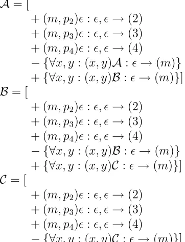
In the example of Figure 4 there are three adaptive actions, namelyA,B andC, which are defined as:

A = [

+ (m, p2)ǫ:ǫ, ǫ→(2) + (m, p3)ǫ:ǫ, ǫ→(3) + (m, p4)ǫ:ǫ, ǫ→(4)

− {∀x, y : (x, y)A:ǫ→(m)}

+{∀x, y : (x, y)B:ǫ→(m)}]

B = [

+ (m, p2)ǫ:ǫ, ǫ→(2) + (m, p3)ǫ:ǫ, ǫ→(3) + (m, p4)ǫ:ǫ, ǫ→(4)

− {∀x, y : (x, y)B:ǫ→(m)}

+{∀x, y : (x, y)C :ǫ→(m)}]

C = [

+ (m, p2)ǫ:ǫ, ǫ→(2) + (m, p3)ǫ:ǫ, ǫ→(3) + (m, p4)ǫ:ǫ, ǫ→(4)

The actionA just defined creates a set of non-adaptive transitions, (because we haveǫbefore and after the colon), in order to return to the original (and correct) path.

ActionA deletes all self-reference adaptive transitions, and creates a new set of transitions that change the deleted ones into corresponding self-reference adaptive transi-tions callingB.

Therefore any other mismatch will perform a similar task with actionB, changing it intoC, and so forth, until the last calling level, when the string is finally rejected.

This sort of sequence of actions creating transitions which call other actions, and replace the existing transitions, allows the automaton to control and ‘count’ existing mis-matches.

If a distancekis needed, we will have to considerkdifferent adaptive actions, so that every action will delete itself when executed, and create another action, the next in sequence, in order to replace it. This way, we may keep track of the distance, as mentioned before, by ‘counting’ the number of actions already performed.

This sort of behavior has some advantages, we can significantly reduce the number of control states needed. Actually there must be one control state, as showed by the example of figure 4, but it can become clearer and more manageable if we create more than one state. Splitting the mistakes from the states, in order to keep a different state to eachk. Doing so allows us to just ‘connect’ or ‘disconnect’ existing transitions, becoming easier to manipulate the state-transition table.

5. Conclusions

This paper presented an alternate way to reduce the number of states of a finite-state automaton, when dealing with approximate string matching. The actual ‘size’ of the automaton model can be reduced to a level very close to the one corresponding to exact string matching.

In fact, the number of initial states is the same of the finite-state automaton for exact match, plus one state. At each mismatch found, the transitions of the automaton are replaced by others, in order to keep control of the number of mismatches, until the number of mismatches reachesk, then no other mismatch will be accepted (because the adaptive transitions are replaced by simple transitions).

However, such a reduction has a price: we will need to replace the transitions at execution time (deleting the existing, and creating others to take their place), despite the fact that it will only be executed when needed. But if we create one state to each level of mistake (k states at all), we will be able manipulate the state-transition table much more easily. In this paper we have not addressed directly the time-complexity of the solution, but we intend to do it.

There are other research studies taking into account this adaptive feature, and we noticed that there are results and practical simulations that uses it, such as [11]. How-ever, they share a common focus, they are connected to the processing of context-free or context-sensitive languages [6].

References

[2] Boyer, R. S., Moore, J. S., A fast string searching algorithm.Comm. ACM20, 10 (1977) 62-72.

[3] Aho, A. V., Corasick, M. J., Efficient string matching: an aid to bibliographic search.

Comm. ACM18, 6(1975) 333-340.

[4] Holub, J., Reduced Nondeterministic Finite Automata for Approximate String Matching.

Proceedings of the Prague Stringology Club Workshop ’96, Czech Technical Univer-sity(August 1996) 19-27.

[5] J. J. Neto, Adaptive Rule-driven Devices - General Formulation and Case Study. CIAA 2001: Proceedings of the 6th International Conference on Implementation and Ap-plication of Automata (2001).

[6] J. J. Neto, Adaptive Automata for Context-Depend-ent Languages. ACM SIGPLAN No-tices29, 9(Sep-tember, 1994) 115-124.

[7] J. J. Neto; C.A. B. Pariente, Adaptive Automata - a revisited proposal.CIAA 2002: Pro-ceedings of the 7th International Conference on Implementation and Application of Automata - Lecture Notes in Computer Science2608(July, 2002) 158-168.

[8] J. Hopcroft, and J. Ullman, Formal Languages and their Relation to Automata. Addison-Wesley. 1969.

[9] H. Lewis, and C. Papadimitriou, Elements of the Theory of Computation. Prentice-Hall. 1998.

[10] Navarro, G., A guided tour to approximate string matching. ACM Computing Surveys 33, 1(March, 2001) 31-88.