INSTITUTO TECNOLÓGICO Y DE ESTUDIOS SUPERIORES DE MONTERREY
PRESENTE.-Por medio de la presente hago constar que soy autor y titular de la obra
, en los sucesivo LA OBRA, en virtud de lo cual autorizo a el Instituto Tecnológico y de Estudios Superiores de Monterrey (EL INSTITUTO) para que efectúe la divulgación, publicación, comunicación pública, distribución, distribución pública y reproducción, así como la digitalización de la misma, con fines académicos o propios al objeto de EL INSTITUTO, dentro del círculo de la comunidad del Tecnológico de Monterrey.
El Instituto se compromete a respetar en todo momento mi autoría y a otorgarme el crédito correspondiente en todas las actividades mencionadas anteriormente de la obra.
A Comparison of Control Schemes for an Articulated 2
Degree-of-Freedom Robot Manipulator Optimized Via Genetic
Algorithms-Edición Única
Title
A Comparison of Control Schemes for an Articulated 2
Degree-of-Freedom Robot Manipulator Optimized Via
Genetic Algorithms-Edición Única
Authors
Jonathan Arriaga González
Affiliation
Tecnológico de Monterrey, Campus Monterrey
Issue Date
2010-05-01
Item type
Tesis
Rights
Open Access
Downloaded
18-Jan-2017 17:42:16
INSTITUTO TECNOLÓGICO Y DE ESTUDIOS
SUPERIORES DE MONTERREY
C A M P U S M O N T E R R E Y
M E C H A T R O N I C S A N D I N F OR M A TI ON T E C H N O L O G I E S G R A D U A T E P R O G R A M
A COMPARISON OF CONTROL SCHEM ES FOR AN ARTICULATED 2 DEGREE-OF-FREEDOM ROBOT MANIPULATOR
OPTIMIZED VIA GENETIC ALGORITHMS
TH E S I S
P R E S E N T E D I N P A R TI A L F U L F I L L M E N T O F T H E R E Q U I R E M E N T S F O R T H E D E G R E E O F
M A S T E R O F S C I E N C E IN I N TE L L I GE N T S Y S T E M S
JO N A T H A N A R R I A G A G O N Z Á L E Z
INSTITUTO TECNOLÓGICO Y D E ESTUDIOS
SUPERIORES D E M O N T E R R E Y
CAMPUS M O N T E R R E Y
M E C H A T R O N I C S A N D I N F O R M A T I O N T E C H N O L O G I E S G R A D U A T E P R O G R A M
A C O M P A R I S O N O F C O N T R O L S C H E M E S F O R A N A R T I C U L A T E D 2 D E G R E E - O F - F R E E D O M R O B O T M A N I P U L A T O R O P T I M I Z E D V I A G E N E T I C A L G O R I T H M S
P R E S E N T E D I N P A R T I A L F U L F I L L M E N T O F T H E R E Q U I R E M E N T S F O R T H E D E G R E E O F
M A S T E R O F S C I E N C E I N I N T E L L I G E N T S Y S T E M S
THESIS
B Y
J O N A T H A N ARRIAGA GONZÁLEZ
A comparison of control schemes for an articulated
2 degree-of-freedom Robot Manipulator optimized
via Genetic Algorithms
by
Jonathan Arriaga Gonzalez
Thesis
Presented to the Graduate Program in Mechatronics and Information Technologies in partial fulfillment of the requirements for the degree of
Master of Science
in
Intelligent Systems
Instituto Tecnológico y de Estudios Superiores de Monterrey
Campus Monterrey
Institute* Tecnológico y de Estudios Superiores de
Monterrey
Campus Monterrey
Mechatronics and Information Technologies
Graduate ProgramThe committee members hereby recommend the thesis presented by Jonathan Arriaga Gonzalez to be accepted as a partial requirement to be admitted to the Degree of
Master of Science, in:
Intelligent Systems
Acknowledgments
This research work was possible with the help of many people I would like to thank.
To my parents Lie. Rodrigo Arriaga and Lie. Imla Gonzalez, and brothers David Arriaga and Azael Arriaga, who taught me to dream and realize these dreams, to be constant, to be honest and to give my best.
To D r . Rogelio Soto for being my advisor, for giving me the chance to attend to the conferences I E E E - S M C 2009 and M I C A I 2009, for bringing me his guidance, suggestions, encouragement, experience, friendship and trust on me all the time in the develop of this research work. To Dr. Jose Luis Meza and Dr. Ernesto Rodríguez for bringing me their valuable experience, support and knowledge. To D r . Manuel Valenzuela, who greatly inspired me to realize this research with his courses, experience, comments, ideas and work.
To D r . Jose Luis Gordillo for accepting me in the eRobots research group and his encouragement and friendship all the time. To Dr. Hugo Terashima for his help to get the scholarship from I T E S M and financial aid from C O N A C y T . To Dr. Ramon Brena, D r . Leonardo Garrido, Dr. Santiago Conant, Dr. Arturo Galvan and Dr. Aldo Diaz who also inspired me in the development of this work through their courses and experience.
To all my classmates and friends.
To I T E S M Campus Monterrey and C O N A C y T for giving me the chance to receive, create and share knowledge and experience.
JON ATH AN AR R I AGA GON Z ALEZ
A comparison of control schemes for an articulated
2 degree-of-freedom Robot Manipulator optimized
via Genetic Algorithms
Jonathan Arriaga Gonzalez
Instituto Tecnológico y de Estudios Superiores de Monterrey, 2010
Thesis Advisor: Dr. Rogelio Soto
Robot manipulators play an important role in actual industrial processes. The trajectory following of robot manipulators is a non-linear problem that still requires much research [34]. This research work focuses on the control of the dynamics of an articulated robot manipulator.
A 2 degree-of-freedom ( D O F ) articulated robot manipulator is simulated, each of the two links of the robot having its respective controller. Two different kind of control objectives for the robot's links are considered, position control and velocity control. Four control schemes for the robot's dynamics were selected. For position, a P I D Controller [24] and a Fuzzy Self-tuning (FST) P I D Controller [14] are considered. On the other hand, for velocity control the F S T P D + Controller [35] and the Fuzzy Sliding Mode ( F S M ) Controller [12, 16, 28] were chosen. Controller's performance and robustness in relevant tasks are evaluated and compared in order to determine which control scheme fits best for each task.
Empirical adjustment of most controller's parameters always depend on the time and tests invested in tuning the controller, it is time consuming and subject to human error. As a fair comparison is intended, controller's parameters are optimized via Genetic Algorithms [22]. W i t h this method, the tuning of parameters is not subtle to human error and the comparison can avoid possible erroneous conclusions.
Contents
Acknowledgments v
Abstract vi
List of Tables ix
List of Figures x
Chapter 1 Introduction 1
1.1 Problem Formulation 2
1.2 Hypothesis 6 1.3 Objectives 6 1.4 Methodology 6 1.5 Document Organization 7
Chapter 2 Artificial Intelligence Methods 8
2.1 Fuzzy Logic 8 2.1.1 Fuzzy Sets and Fuzzy Subsets 8
2.1.2 Linguistic Variables 9 2.1.3 Fuzzifiers and Defuzzifiers 11
2.1.4 Fuzzy I F - T H E N rules 12 2.1.5 Fuzzy Inference Engine 13 2.1.6 Fuzzy Processing of Variables 14
2.2 Genetic Algorithms 14 2.2.1 The Algorithm Description 15
2.2.2 Simple example of Genetic Algorithm 17
Chapter 3 Robot Mechanics 21
3.1 Robot Kinematics 21 3.2 Robot Dynamics 22
3.2.3 Dynamic model of Robot Manipulators 27 3.2.4 Dynamic model of a 2 D O F Robot Manipulator 29
3.2.5 Dynamic model parameters 30
Chapter 4 Controller design 32
4.1 Position Controllers 33 4.1.1 P I D Controller 33 4.1.2 Fuzzy Self-Tuning P I D Controller 34
4.2 Velocity Controllers 36 4.2.1 Fuzzy Self-Tuning P D + Controller 36
4.2.2 Fuzzy-Sliding Mode Controller 39
Chapter 5 Simulation Results 46
5.1 Position Controllers 47 5.1.1 Model Reference for Position Controllers 48
5.1.2 Simulation Results for the P I D Controller 49 5.1.3 Simulation Results for the F S T P I D Controller 55
5.1.4 Position Controllers Comparison 57
5.2 Velocity Controllers 60 5.2.1 Simulation Results for the F S T P D + Controller 61
5.2.2 Simulation Results for the F S M Controller 66
5.2.3 Velocity Controllers Comparison 68
Chapter 6 Conclusions 71
6.1 Discussion about Position Controllers 71 6.2 Discussion about Velocity Controllers 72 6.3 Contributions of this research work 73
6.4 Further Work 73
Appendix A Final Value of Parameters modified by the G A 74
A . l Final Values for Parameters of Controllers 74 A.2 Sliding Surface of the F S M Controller 82 A . 3 P I D with Unsaturated Torque Signal 88
Bibliography 90
List of Tables
2.1 Initial random population 19 2.2 Population after the first cycle 19 5.1 Parameters of the G A used to optimize the P I D controllers 49
5.2 Parameters adjusted by the G A for the P I D controller of each link. . . 49
5.3 Parameters that define a F L T 55 5.4 Rules selected fromzyxwvutsrqponmlkjihgfedcbaZYXWVUTSRQPONMLKJIHGFEDCBA RuleOrder 56 5.5 Parameters of the G A used to optimize the F S T P I D controllers 56
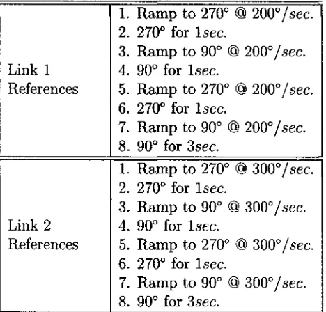
5.6 Performance Comparison of Position Controllers 60 5.7 Parameters of the G A used to optimize the F S T P D + controllers. . . . 61
5.8 References for velocity controllers in the optimization process 62 5.9 References for velocity controllers in performance tests 63 5.10 References for velocity controllers in robustness tests 65 5.11 Parameters adjusted by the G A for the F S M controllers 67 5.12 Parameters used by the G A to optimize the F S M controllers 67
5.13 Performance Comparison of Velocity Controllers 69 A . l Final Values for the P I D Controller of Link 1 77 A.2 Final Values for the P I D Controller of Link 2 77 A.3 Final Values for the F S T P I D Controller of Link 1 78 A.4 Final Values for the F S T P I D Controller of Link 2 79 A.5 Final Values for the F S T P D + Controller of Link 1 81 A.6 Final Values for the F S T P D + Controller of Link 2 81 A.7 Final Values for the F S M Controller of Link 1 83 A.8 Final Values for the F S M Controller of Link 2 84
List of Figures
2.1 Triangular and Trapezoidal M F s 10
2.2 M F s forzyxwvutsrqponmlkjihgfedcbaZYXWVUTSRQPONMLKJIHGFEDCBA speed. 10
2.3 Example of fuzzy processing of variables 14
2.4 Fitness assignment to a population of n individuals 16
2.5 Flow chart diagram of steps the Genetic Algorithm performs 17
2.6 Function f(x) = y/x 18
3.1 Sketch of a 2 D O F Robot Manipulator 24
4.1 P I D block diagram 34 4.2 F S T P I D block diagram 35
4.3 F L T parameters 35 4.4 F S T P D + block diagram 39
4.5 Sliding surface in a phase plane 40 4.6 Discontinuous term of equation 4.26 42 4.7 Presence of chattering as the result of control switching 42
4.8 F S M block diagram 43 4.9 F S M controller parameters 43
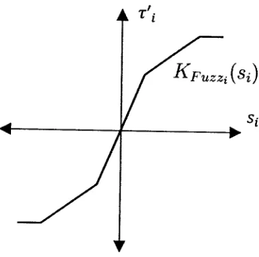
4.10 Possible shape of function Kpuzziisi) 45
5.1 Fitness assignment for optimization of controllers 47 5.2 Methodology applied to compare Position controllers 48 5.3 P I D with optimized parameters. Response of: a) link 1; b) link 2. . . . 50
5.4 P I D performance test. Response of: a) link 1; c) link 2. Torque for b)
link 1; d) link 2 52 5.5 P I D robustness test. External perturbation for: a) link 1; b) link 2.
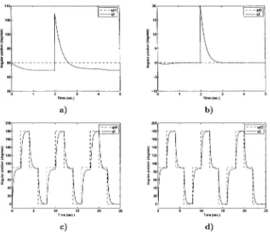
Parametric variations for: c) link 1; d) link 2 54 5.6 F S T P I D with optimized parameters. Response of: a) link 1; b) link 2. 57
5.7 F S T P I D performance test. Response of: a) link 1; c) link 2. Torque for
b) link 1; d) link 2 58 5.8 F S T P I D robustness test. External perturbation for: a) link 1: b) link
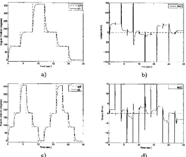
5.9 Methodology applied to compare Velocity controllers 61 5.10 F S T P D + with optimized parameters. Response of: a) link 1; b) link 2. 62
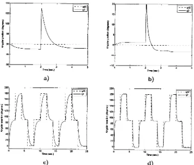
5.11 F S T P D + performance test. Response of: a) link 1; c) link 2. Torque
for b) link 1; d) link 2 64 5.12 F S T P D + robustness test. External perturbation for: a) link 1; b) link
2. Parametric variations for: c) link 1; d) link 2 66 5.13 F S M with optimized parameters. Response of: a) link 1; b) link 2. . . 68
5.14 F S M performance test. Response of: a) link 1; c) link 2. Torque for b)
link 1; d) link 2 69 5.15 F S M robustness test. External perturbation for: a) link 1; b) link 2.
Parametric variations for: c) link 1; d) link 2 70 A . l M F s of F L T s of F S T P I D Controller for link 1 75 A.2 M F s of F L T s of F S T P I D Controller for link 2 76 A . 3 M F s of F L T s of F S T P D + Controller for link 1 77 A.4 M F s of F L T s of F S T P D + Controller for link 2 80
A.5 M F s of the F S M Controller for link 1 82 A.6 M F s of the F S M Controller for link 2 82
A . 7 FunctionzyxwvutsrqponmlkjihgfedcbaZYXWVUTSRQPONMLKJIHGFEDCBA KFuzzi(s\) 83
A.8 Function KFUZZ2(
S2) 83
A.9 Phase plane response of the F S M for: a) link 1; b) link 2 85 A . 10 Phase plane response of the classical Sliding Mode for: a) link 1; b) link
2 85 A . 11 F S M test. Response of a) link 1; b) link 2. Torque for: c) link 1; d) link
2 86 A . 12 Classical Sliding Mode. Response of: a) link 1; b) link 2. Torque for: c)
link 1; d) link 2 87 A . 13 P I D with unsaturated torque. Response of: a) link 1; b) link 2. Torque
Chapter 1
Introduction
Robot manipulators are commonly used in industrial process to develop tasks like painting, pick and place, arc welding and others. Actually, industrial robots are capable to develop a great variety of activities with high precision and repeatability. However, research about robotics is relevant given that there are still many applications that commercial robots are unable to perform correctly, like handling of fragile objects and imitation of human moves. The trajectory following of a robot manipulator is a non-linear control problem that still requires much research and is a very important field for production process. It is also an interesting control problem from the academic point of view.
This thesis focuses on the control of the dynamics of robot manipulators. The desired control objective is to make the manipulator asymptotically follow a given trajectory within a finite interval of time. This objective is not possible in general since asymptotic stability can be achieved only as time approaches to infinity [34] from the theoretical point of view.
Actual industrial robots have gears in its joints which transmit power from the actuators. When gear ratio is big enough, the robot's dynamics simplifies greatly to the point that the non-linearities can be neglected [34]. The robot's dynamics is given thus only by the dynamics of the actuators. The counterpart of using gears is that the mechanical complexity of the system increases and the mass does as well.
Thus, if no gears are used, the primary difficulty for the control of the robot's dy-namics is that the robotic system is highly non-linear and presents inherently unknown dynamics [31]. A non-linearity in a system is a non-proportional relation between cause and effect. Physical systems are inherently linear, thus all control systems are
non-linear from a certain point of view. Non-non-linearities can be classified aszyxwvutsrqponmlkjihgfedcbaZYXWVUTSRQPONMLKJIHGFEDCBA inherent (natural)
and intentional (artificial) [5]. Inherent non-linearities are those which naturally come with the system's hardware and motion. Centripetal forces in rotational motion and Coulomb friction between contacting surfaces are examples of non-linearities.
exam-pie, when a robot takes an object, due to the object's mass, the apparent mass of the robot's last link is increased. The other links are affected by this parameter change because the robot is a linked mechanism. Adaptable control laws are heavily studied with the aim to minimize the perturbations with time.
If a controller that handles well all this issues is developed along with the needed actuators, it could be possible to design lighter and faster robots, with less or without gears. However, the mechanical design of robots is beyond the scope of this document, which focuses mainly on the study of the control of robot's dynamics.
W i t h the speed of actual processors many complex control techniques are possi-ble to be implemented. Actual actuators have also many capabilities which weren't available when robots from the last two decades were designed, thus the design of even actual robots has limitations not valid for today's technology. In the research presented in this document, performance of two controllers of the same kind for the same task is compared. A simulation model of a 2 degree-of-freedom (DOF) articulated robot is used to compare the different control schemes and decide which performs better for different kind of tasks.
1.1 Problem Formulation
When controlling the dynamics of articulated robot manipulators, the principal problem is the inherent linearities in the system. The logical choice when a non-linear system will be controlled is to use a non-non-linear controller which absorbs the non-linearities; while if the system is linear, then a linear controller would be the best choice. If the operating point of a given control system is small and the non-linearities are smooth, the control system may be approximated by a linear system with good accuracy.
Many of the most common controllers are linear because its application does not require improved performance or the operating point can be approximated as a linear system. A n articulated robot manipulator is a non-linear system and its operating point is the whole range of movement, therefore its dynamics cannot be approximated
to a linear system [34]. From this point in the document, the termzyxwvutsrqponmlkjihgfedcbaZYXWVUTSRQPONMLKJIHGFEDCBA robot manipulator
will refer to articulated robot manipulator.
As a robot manipulator is subject to an environment with high variability, inter-acts with objects of different sizes and weights and its parameters can change with time as the robot ages. The dynamic model of a robot manipulator can be derived mathe-matically or by analyzing system data, but uncertainties of the actual real system with respect to the system model will always exist.
of the controller, and second, how tozyxwvutsrqponmlkjihgfedcbaZYXWVUTSRQPONMLKJIHGFEDCBA set numerical values of the controller parameters [39]. The first problem can be solved based in the approximated system model and the
task type. For the second problem, depending on the controller there may be a method to adjust its parameters.
Controlling the dynamics of robot manipulators means to make the robot's links asymptotically approach to a reference. It is an interesting problem and represents some challenges in the design of the controller's structure and optimization due to its non-linearities and model uncertainties.
For robot manipulators, position tasks means regulating the system in a static position reference. Velocity tasks, in the other hand, means tracking of position trajec-tories. The tracking problem can be defined as follows [5]: Given a non-linear dynamics system and a desired output trajectory, find a control law for the input such that start-ing from any initial state within a bounded region, the trackstart-ing errors go to zero while the whole state x remains bounded.
Velocity controllers are defined as follows [10]: Assume that joint position q and joint velocity q are available for measurement. Let the desired joint position qd be a
twice differentiable vector function. The controller will determine the actuator torques r in such a way that the following control aim be achieved
(1.1) The control system is said to be globally asymptotically stable if the control aim is guaranteed irrespective of the robot initial configuration q(0) and q(0).
For this research, two different controllers will be optimized for position tasks: P I DzyxwvutsrqponmlkjihgfedcbaZYXWVUTSRQPONMLKJIHGFEDCBA Controller The conventional P I D controller is widely used in industrial process
control because of its simplicity and its rather satisfactory performance. This controller was introduced in 1922 as a three-term controller [24]. It grow popular and was heavily analyzed to date. It is commonly used in applications in which the process parameters are well known and do not vary substantially [14].
controller, which is known as Fuzzy Self-tuning (FST) P I D controller. Stability about this controller has been studied in [36, 21]. In [22] Membership Func-tions (MF) for this controller have been optimized via Genetic Algorithms and compared against an empirical tuning.
Similarly, for velocity tasks two controllers will be considered:
Fuzzy Self-Tuning P D + Controller This controller was introduced first in [17] in 1998 as Fuzzy Self-tuning torque Control based in the Computed-torque Method [29]. It was later handled as Fuzzy P D + in [35], which is also based in the controller introduced in [10] known as P D + . The structure of P D + control consists of a linear P D feedback plus a specific compensation of the robot dynamics. In the Fuzzy P D + control scheme, the gains of the P D + are allowed to vary according to a fuzzy logic system which depends on the robot state. This is an important ingredient to deal with practical specifications such as keeping asymptotically the tracking error within prescribed bounds without saturating the actuators. Stability for this controller is analyzed in [17, 35, 33].
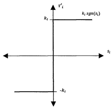
Fuzzy Sliding Mode Controller The Fuzzy-Sliding Mode (FSM) Controller has the characteristics of both a fuzzy logic controller and a variable structure controller (VSC) or also known as sliding mode controller. It was introduced in 1992 in [12, 16] and was further studied in [28]. The F S M C has a fuzzy-sliding motion similar to the conventional sliding motion of the V S C . In the F S M C the switch-ing hyper plane is a fuzzy set, while in the slidswitch-ing mode controller is a crisp set. Membership functions and fuzzy rules can easily be determined to prespecify the behavior of control system. In the conventional sliding mode controller, when the system enters into sliding mode, the state trajectories of the controlled system will be kept on a specified switching hyperplane. Due to the sampling action of digital implementation, delay of switch device and its operation at discrete instants, a sliding mode controller may have chattering. This phenomenon is undesirable in most control applications because high frequency components in the system not considered in the model could be excited and make the system unstable. One of the principal motivations to develop the F S M C was the attenuation of chatter-ing. A simulation of a 6 D O F robot manipulator implementing this controller is reported in [3].
P I D controllers, which are very popular and effective for industrial applications but its performance depends heavily on the operating parameters of the system. Once these parameters change, a significant amount of effort is required to manually tune the P I D controllers [22].
A n approach based in Genetic Algorithms (GA) is considered for this task. G A s have been applied to control problems in approximating the system's model and for the design and optimization of the controller for the system. In [39] a Genetic Algorithm is implemented as an estimator for discrete time and continuous systems. Genetic Algorithms are used in [11] to estimate both continuous and discrete time systems and for identifying poles and zero or physical parameters of a system, in order to design an adaptive controller in combination with a pole placement scheme.
A comparison of Fuzzy Control against P I D Control for a Position and Force Control of a Robot hand is presented in [8] and resulted that the Fuzzy Controller outperformed the P I D Controller in tests of pure position control and pure force control. In that paper, both controllers were empirically adjusted, which lacks of a formal proof to determine if one controller has a better performance than another one. A P I D controller has been successfully optimized with a G A comparing this optimization with that of a Simulated Annealing (SA) method and empirically adjusted settings in [13], the G A outperformed the optimization by SA and the empirical method. The last comparison is much better than the first one because the tuning of parameters in this case is not subtle to human error, which could have a negative effect in the controller's performance.
Therefore, G A s will be used to optimize the controller's parameters to work in relevant operating points of the robot's links. After optimization, controller's perfor-mance criterions will be measured and compared to determine which fits best for each kind of task. It is always important to make fair comparisons, in this case conditions of the system and design of controllers must be the same. Conditions of the system can easily be simulated to be the same, the difficulty relics in performing a fair tuning of controllers. Most controllers can have excellent performance if well tuned, while if tuning is poor then performance is also.
1.2 Hypothesis
The principal hypothesis is that controllers for the dynamics or robots manipula-tors can be successfully optimized by Genetic Algorithms. Different controller schemes can then be compared fairly when optimized by this method. The comparison and the parameters of the controllers optimized provide relevant knowledge about the control of the system.
1.3 Objectives
The first objective of this research work is to optimize the proposed controllers to develop specific tasks. Once the controllers have been optimized, a comparison of performance criterions will be made. Optimization before performing a comparison is vital because is the most important part of the design. A controller is not useful if it is not well tuned, but is very useful if all parameters are set so the system develops the specified task.
A particular objective, regarding to position controllers is to determine if a non-linear controller handles the system much better than a non-linear controller. This will tell if the extra controller-complexity makes a real difference or is enough with a linear well-tuned controller .
1.4 Methodology
Given a physical system to be controlled, a common procedure for control design is as follows, with possibly a few iterations [19]:
1. Specify the desired behavior, and select actuators and sensors. 2. Model the physical plant by a set of differential equations. 3. Design a control law for the system.
4. Analyze and simulate the resulting control system. 5. Implement the control system in hardware.
For this thesis, only steps 1 to 4 are followed for each controller, implementation of the control system is left as a future work. Steps 3 and 4 are done for each of the 4 controllers considered to analyze.
having each controller designed and optimized, a comparison of performance criterions will determine which controller is better for each particular task.
Steps for the optimization and performance evaluation process are listed below: 1.zyxwvutsrqponmlkjihgfedcbaZYXWVUTSRQPONMLKJIHGFEDCBA Optimization. In this step the parameters for the controller of each link are
optimized with the G A .
2. Performance tests. Once optimized, both controllers for each task are tested in normal operation conditions.
3. Robustness tests. The robustness of each controller is evaluated by modifying the operation conditions for which the controller was optimized.
1.5 Document Organization
Chapter 2
Artificial Intelligence Methods
In this section two popular Artificial Intelligence methods are described. One is Fuzzy Logic, a method to represent knowledge and has been used broadly in control, decision-making techniques, prediction, etc. The other is Genetic algorithms ( G A ) , which is an optimization method based in the mechanics of natural evolution of a population.
In the early 1960's, Lofti A . Zadeh from the University of California at Berkley introduced the idea and concept of grade of membership for the elements of a set. In 1965, he published his seminar paper on fuzzy sets [40] which lead the emergence of the fuzzy logic technology. The first fuzzy logic controller was published by [20], used to control a simple dynamic plant.
Fuzzy logic is an extensively studied field, many concepts and many applications have been developed. In this section a brief explanation of the most important concepts for understanding fuzzy logic most of these reported in [2].
2.1.1 Fuzzy Sets and Fuzzy Subsets
A fuzzy set is a generalization to classical set where the elements have degrees of
membership. A fuzzy set is characterized by having a set of elements and azyxwvutsrqponmlkjihgfedcbaZYXWVUTSRQPONMLKJIHGFEDCBA membership
function ( M F ) that maps these elements of a universe of discourse to their corresponding
membership values. The M F of a fuzzy set A is denoted by HA- The logic operators of intersection and union have multiple choices for the fuzzy conjunction (AND) and the fuzzy disjunction (OR) operators.
A n ordinary subset A of a set X can be identified with a function X —> {0,1} from X to the 2-element set {0,1} as follows
2.1 Fuzzy Logic
This function is called the characteristic function.
Different from ordinary subsets,zyxwvutsrqponmlkjihgfedcbaZYXWVUTSRQPONMLKJIHGFEDCBA fuzzy subsets ofzyxwvutsrqponmlkjihgfedcbaZYXWVUTSRQPONMLKJIHGFEDCBA X can have varying degrees of membership from 0 to 1. Using fuzzy subsets, the value of A(x) is thought as the
degree of membership of x in A . This function is called membership function of A
and can be expressed aszyxwvutsrqponmlkjihgfedcbaZYXWVUTSRQPONMLKJIHGFEDCBA HA : X —> [0,1]. A n special case is when the M F only takes values 0 or 1, A is known i n this case a crisp subset of X.
Commonly the set X is called the universe of discourse. Since data is generally numerical, the universe of discourse is most often an interval of real numbers. The shape of a M F depends on the notion the set is intended to describe and on the particular application involved. Common M F s for control applications are triangular, trapezoidal, Gaussian and sigmoidal Z- and S-functions.
Triangular M F are used in applications very often, see figure 2.1. Equation 2.2 characterizes the degree of membership of x in this kind of M F . Graphical represen-tations and operations with these fuzzy sets are simple. A triangular M F A with end points (a, 0) and (6,0), and high point (c, a) is defined by:
For the case of trapezoidal M F , end points (a, 0) and (6,0), and high points (C , Q) and (d, a) define a trapezoidal M F A as follows:
M F s are useful for processing numeric input data. A wider explanation of fuzzy subsets can be found in [25].
2.1.2 Linguistic Variables
When a variable is described with numbers as values, it can be formulated with math theory. But when a variable takes words as values, there isn't a formal structure to formulate the problem with classic math theory [15]. The linguistic variables concept was introduced in order to provide a formal structure to deal with words as values. Linguistic terms are useful for communicating ideas and knowledge with human beings, is the most important element in the representation of human knowledge.
Figure 2.1: Triangular and Trapezoidal M F s .
Figure 2.2: M F s forzyxwvutsrqponmlkjihgfedcbaZYXWVUTSRQPONMLKJIHGFEDCBA speed.
"high" and "low" are linguistic values. A linguistic variable is the equivalent of a symbolic variable in A I and a numeric variable i n science and engineering. In general, the values of a linguistic variable can be linguistic expressions of terms and modifiers such as "very", "more" and connectives such as "and", "or".
For example, the velocity of a car is x, which can take values in the interval [0,zyxwvutsrqponmlkjihgfedcbaZYXWVUTSRQPONMLKJIHGFEDCBA Vmax], where Vmax is the car maximum velocity. Two M F s are defined "s/ou/' and
"fast' within [0, Vmax] as shown in 2.2. If x is considered as a linguistic variable, it can
take values as "s/otu" and "fast'. Thus, it can be said that "x is slouP or "x is fas?.
Formally, a linguistic variable is characterized by (X, T, U, M), where:
X is the name of the linguistic variable. From figure 2.2, X is the car speed.
MzyxwvutsrqponmlkjihgfedcbaZYXWVUTSRQPONMLKJIHGFEDCBA is a semantic rule relating each linguistic value i n T with a fuzzy subset i n U. From the last example, M relates T= slow, fast with the M F s in figure 2.2.
2.1.3 Fuzzifiers and Defuzzifiers
The fuzzification process is defined as a mapping from a real-valued point x* G U C Rn to a fuzzy set A' i n U. While designing a fuzzifier, one should consider that
the input is at the crisp point x*, the fuzzy set A' should have a large membership value at x*. If the input to the fuzzy system is corrupted by noise, it is desirable that the fuzzifier should suppress the noise. Maybe one of the most important points when designing a fuzzifier is the computations involved in the inference engine. If the fuzzifier is ruled by a complex formula then performance will be greatly affected, furthermore the knowledge with a complex function will be harder to understand by a human being than when using a simpler function.
In [15], three fuzzifiers are proposed:
Singleton fuzzifier The singleton fuzzifier maps a real-valued point x* G U into a fuzzy singleton A' in U, which has a membership value 1 at x* and 0 at other points int t/; it is expressed as
(2.5) where 6j are positive parameters and * describes the t-norm (described i n [15, 25]), which is usually an algebraic product or rain product. In order to use trapezoidal M F s (which are an extension of triangular M F s ) , little changes should be implemented i n the last equation.
Gaussian fuzzifier The Gaussian fuzzifier maps x* £ U into a fuzzy set A' in U
which has the following Gaussian M F :
U is the physical domain i n which X can take quantitative values. From figure 2.2,
(2.4)
Triangular fuzzifier The Triangular fuzzifier maps x* € U into a fuzzy set A' in U
(2.6) This fuzzifier method is broadly used in many applications, however the applica-tion described i n chapter 5 only uses trapezoidal and singleton fuzzifiers.
ThezyxwvutsrqponmlkjihgfedcbaZYXWVUTSRQPONMLKJIHGFEDCBA defuzzification process is a mapping from fuzzy set B' i n VzyxwvutsrqponmlkjihgfedcbaZYXWVUTSRQPONMLKJIHGFEDCBA C R to a crisp point y* G V. In other words, the defuzzifier specifies a point in V that best represents
the fuzzy set B', which is similar to the mean value or a random variable. The fuzzy set B' is defined in a special way and there are a number of methods to determine its representing point. T h e design of the fuzzy subset B' along with the defuzzification process should consider the same points as when designing the fuzzification process.
Also in [15] the center of gravity defuzzifier, center average defuzzifier, maximum defuzzifier are defined. For the application i n this document, only the center average defuzzifier process is reported.
Center average defuzzifier A s the fuzzy set B' is the union or intersection of M
fuzzy sets, an approximation of the centers of the M fuzzy sets with the weights equal the heights of the corresponding fuzzy sets. Let y~l be the center of the I'th
fuzzy set and wi be its height, the center average defuzzifier determines y* as:
This defuzzifier is the most commonly used defuzzifier in fuzzy systems and fuzzy control. It is computationally simple and intuitive plausible, small changes in y~~l
and wi result i n small changes in y*.
Fuzzy systems are knowledge-based systems or rule-based systems. The core of a fuzzy system is a knowledge base composed of fuzzy I F - T H E N rules. A fuzzy I F - T H E N rule is a relation that transforms conditions about linguistic variables to conclusions.
The following is an example of a fuzzy I F - T H E N rule [15]:
in which words "high" and "/ess" are characterized by M F s . Fuzzy rules are com-monly generated from a human expert in the system or from knowledge obtained while operating the system.
(2.7)
2.1.4 Fuzzy I F - T H E N rules
IF velocity of car is high
The main feature of this kind of knowledge representation is its partial matching capability that enables an inference even when the rule conditions are partially satisfied. To infer a conclusion in a fuzzy rule, the conditions based on the match degree of the input data and the consequent are combined. The higher is the matching degree, the closer is the inferred conclusion to the consequence of the rule.
2.1.5 Fuzzy Inference Engine
A typical rule base is of the form
(2.8)
A common interpretation forzyxwvutsrqponmlkjihgfedcbaZYXWVUTSRQPONMLKJIHGFEDCBA Rj is a fuzzy relation X x U. This means that when the input is x, the degree to which a value u € U is consistent with the meaning of Rj
is
where T is some t-norm [25]. Thus, Cj is a fuzzy subset of X x U. For a given input
x, Cj induces a fuzzy subset of U
This implies that the output of each rule Rj is a fuzzy subset of U. The Mamdani method [20] uses the minimum of the t-norm:
(2.9)
(2.10)
(2.11)
(2.12) Having translated each rule Rj into CJ, the next task is to fuse all the rules together. The problem is that given N fuzzy subsets, C f , • • •, C% of U, it is needed to combine them to produce and overall output. What is wanted is a single fuzzy subset of U from the CJ, j = 1, • • •, N. The Mamdani method to accomplish this task is for each x G X = Xx x • • • x Xn, this gives the fuzzy subset
(2.13) of U. This last equation is known as Mamdani synthesis.
The overall output is, for each x, a fuzzy subset Cx of U. The meaning of Cx is
Figure 2.3: Example of fuzzy processing of variables.
In most control applications, a single numerical (crisp) output is neededzyxwvutsrqponmlkjihgfedcbaZYXWVUTSRQPONMLKJIHGFEDCBA u* = u*(x) for the control law. A crisp output is obtained from Cx using any of the defuzzification
methods described above.
2.1.6 Fuzzy Processing of Variables
The fuzzy processing of crisp variables can be summarized as follows:
Fuzzification Mapping from a real-valued point (crisp point) to an input fuzzy set in the universe of discourse.
Rule-Based Inference Transformation of input fuzzy sets into output fuzzy sets by means of a set of rules and an inference engine.
Defuzzification Mapping from output fuzzy sets to a real-valued point.
The process above summarized is illustrated in figure 2.3. This figure shows an example of a single-input single-output fuzzy system, however, the number of input and output variables a fuzzy system can process is not limited.
2.2 Genetic Algorithms
measure. Genetic algorithms are no simple random walk, they exploit the historical information to speculate on new search points with expected improved performance.
The principal differences of G A s from more normal optimization and search pro-cedures are:
• G A s work with a coding of the parameters, not the parameters themselves. • G A s perform a parallel search, exploring many points in the search space at the
same time.
• G A s use only the result from the objective function to guide the search. • G A s use probabilistic transition rules, not deterministic rules.
2.2.1 The Algorithm Description
The core of the G A is the codification of the solution to the problem, usually han-dled as a binary string of finite length called chromosome. Each solution is known as an individual, there is a number of individuals (solutions) that compose a
pop-ulation. Every cycle of the G A , individuals are evaluated with a fitness function and with some operators (that will be described next) a new population or offspring is created. The cycles in which a new population is created are called generations.
So, the G A works with a population of solutions that explore the search space at the same time (within a generation), therefore is said that G A s perform a parallel search, regardless of the fact that only one solution is evaluated at a time.
To run a G A , an initial population is needed, it can be random (setting every bit of the chromosome of every individual randomly to 0 or 1) or defined, maybe as the last population of a previous run. Within a population, every individual is codified into a string representing its chromosome.
A codification withzyxwvutsrqponmlkjihgfedcbaZYXWVUTSRQPONMLKJIHGFEDCBA real numbers has also been developed and implemented in [23], the best representation is the one which is more natural to the problem. Computer languages in which individual bits cannot be accessed the real codification is encouraged. However, there is an option to this case, the virtual gene genetic algorithm (vgGA) [38]. In the v g G A , traditional crossover and mutation are implemented as arithmetic functions. This implementation allows the generalization to virtual chromosomes of alphabets of any cardinality. This codification is more efficient than using an integer number to represent a single bit, in terms of computer memory.
Figure 2.4: Fitness assignment to a population ofzyxwvutsrqponmlkjihgfedcbaZYXWVUTSRQPONMLKJIHGFEDCBA n individuals.
generations with the same fitness function. This sub procedure is illustrated in figure 2.4.
Having received an evaluation with the fitness function, individuals arezyxwvutsrqponmlkjihgfedcbaZYXWVUTSRQPONMLKJIHGFEDCBA
repro-duced in a way that those with higher fitness receive more copies and those with lower fitness receive less copies. A popular method for selecting individuals to repro-duce based in its fitness is roulette-wheel selection. In roulette-wheel selection, fitness for all individuals compose a wheel with every individual having a piece of the wheel representing its relative fitness with respect to the total population. A pointer points randomly to some place in the wheel and the chosen individual receive a copy in a mating pool. This is performed a number of times equal to the size of the population.
After the selection process, stronger individuals (with higher fitness) are more likely to have more copies in the mating pool than the weaker ones. Once the mating pool is created each copy of each individual mates with another one chosen randomly. A crossing point is selected within the string bits for each mate to perform crossover after that point, this is called single-point crossover. Multiple-point crossover has been analyzed in [37], results suggest that two-point crossover performs better than single-point crossover. W i t h crossover, a new offspring is generated, two new individuals for the next generation are created from two individuals in the current generation. Crossover of two individuals with cross point after the second bit is illustrated below.
Before crossover After crossover
00100 00111 11111 ~* 11100
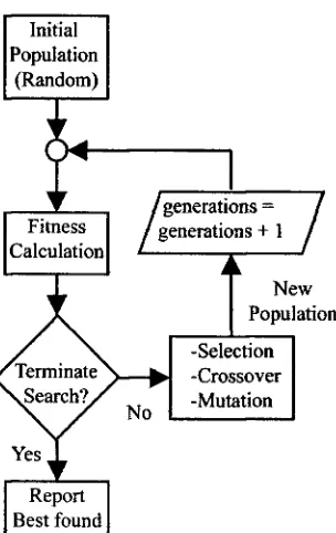
Figure 2.5: Flow chart diagram of steps the Genetic Algorithm performs.
This is a brief description of G A s , a pseudo code of the whole algorithm is rather complicated. Instead, a flow chart diagram of a simple G A is illustrated in figure 2.5. A pseudocode version has already been reported in [6].
2.2.2 Simple example of Genetic Algorithm
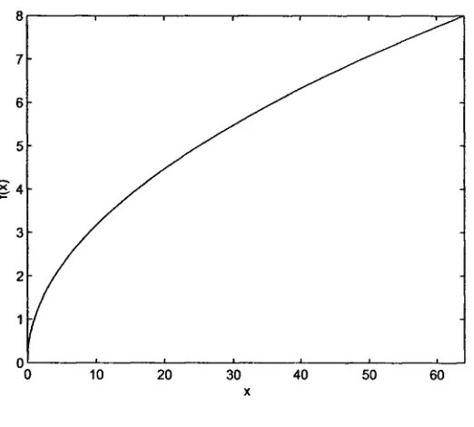
In this section a G A is followed step by step to illustrate it's mechanics. First, consider the functionzyxwvutsrqponmlkjihgfedcbaZYXWVUTSRQPONMLKJIHGFEDCBA f(x) = \fx, when x 6 [1 64] illustrated in fig. 2.6. The G A will try to find the value for x that maximizes the function f(x).
If the shape of the function is not known or where the maximum value can be found, a wide range for the involved variables must be chosen in order to let the G A find the optimal values for that function. This is a weak point for the G A , it can only explore points within the given range of variables.
As the G A only works with binary numbers, x must be codified in a binary string, which for this example will be of length 4. The four digit string can represent values from 0 (0000) to 16 (1111), these digits must be decodified to transform them into valid values for x. The following expression is used for the decodification of the binary unsigned integer representation of the string.
Figure 2.6: FunctionzyxwvutsrqponmlkjihgfedcbaZYXWVUTSRQPONMLKJIHGFEDCBA f(x) =
werezyxwvutsrqponmlkjihgfedcbaZYXWVUTSRQPONMLKJIHGFEDCBA d(i) is the decodified value of the integer representation of the string z, xm a x
and xmin are the limits for x and I is the length of the string. For example, the string
(1111), with unsigned integer given by i = 16 is decodified into d(i) — 64 using equation 2.14. This is one of many ways to decode a string, depending on the application other methods for decodification can be used.
Until now, only the codification and decodification methods have been defined. The following step is to create a population of individuals, for this case the population will be composed only by four individuals. The population is created by giving each individual a string with each bit value randomly selected as 0 or 1. Table 2.1 illustrates the initial population, values for fitness are obtained by evaluating each individual (which is an instance of x) with the function f(x). The parameter |&j is the probability of selection for that individual, the higher the value for this parameter, the higher will be its probability to obtain a copy in the mating pool. The expected count ~ is an estimate of the number of copies each individual will have in the mating pool after selection.
Table 2.2 shows the population after the first cycle. Cross points were randomly selected and resulted in 3 for the first mate and 2 for the second mate. Mutation is set to 2% and acts along all bits in the chromosomes of all individuals, in this case only the last bit in the chromosome of the last individual was mutated. It is known from figure 2.6 that the maximum of f(x) will be when x = 64 by string 1111, having fitness equal to f(x) = 8.
Table 2.1: Initial random population.
#
Parents (Last Gen.) Individual String i d{i) m JL.E / k f
Actual Count
1 - 1110 14 59.8 7.73 0.35 1.38 2
2 - 0101 5 22.0 4.69 0.21 0.84 1
3 - 1001 9 38.8 6.22 0.28 1.12 1
4 - 0011 3 13.6 3.68 0.16 0.66 0
Sum Average 22.32 5.58 1 0.25 4 1 4 1
Table 2.2: Population after the first cycle.
#
Parents (Last Gen.) Individual String i d(i) m £ / h fIf the solution of the problem requires an improved accuracy for the involved vari-ables, the codifying strings for those variables must be larger and a bigger population must be used. If the evaluation of every individual is costly and the solution requires a good resolution, the algorithm run will take much time. Knowledge about the opti-mal solution of the problem and its behavior can improve the algorithm's performance greatly.
In the second step the G A has already found the optimal with only eight
eval-uations of the objective function out of the 16 possible valueszyxwvutsrqponmlkjihgfedcbaZYXWVUTSRQPONMLKJIHGFEDCBA x can be decodified into. This may not sound surprising because the example is very simple, but for bigger
problems with solutions codified in larger strings, the G A works with higher efficiency. It is known for advance which is the optimal value of x for the fitness function f(x)
Chapter 3
Robot Mechanics
3.1 Robot Kinematics
Manipulator-type robots have multiple D O F , are three dimensional, are open loop and are chain mechanisms. Kinematics analysis of robots have been extensively studied and reported in the literature. Analysis for robot manipulators are can be found in [26, 34, 9].
For a kinematic analysis, a three-dimensional reference frame is placed in the base
of the robot, denoted by the coordinateszyxwvutsrqponmlkjihgfedcbaZYXWVUTSRQPONMLKJIHGFEDCBA [x y z]T. Links are numbered consecutively
from the base (link 0) to the end effector (link n). Joints are contact points between the links and are numbered in such a way that joint i connects the links i and i — The axis of motion of joint i is assigned to the z axis and identified by z%. The generalized articular coordinate, denoted by is the angular displacement around z, if joint i is rotational, or the lineal displacement over z; if joint i is translational.
Articular positions for every link are measured with sensors placed in the actuators, which are commonly located in the joints. For a n D O F robot, the articular positions vector q will have n elements:
(3.1) The position and orientation of the end effector of the robot is essential for most of the applications because is the element that performs the desired task. This position and orientation is expressed in terms of the reference coordinate frame located in the base of the robot. The x vector of Cartesian positions which contains coordinates and angles can be written as follows:
(3.2) where m < n.
that three components of thezyxwvutsrqponmlkjihgfedcbaZYXWVUTSRQPONMLKJIHGFEDCBA x vector refer to the position and the other three to the orientation of the end effector.
The forward kinematics model of a robot describes the relationship between the articular positionszyxwvutsrqponmlkjihgfedcbaZYXWVUTSRQPONMLKJIHGFEDCBA q and the position and orientation x of the robot's end effector, as represented by eq. 3.3.
(3.3) This model can be obtained following a methodology and involving simple trigono-metric expressions and identities. The inverse kinematics model is just the inverse relation of the forward kinematics model as shown below:
(3.4) Different from the forward kinematics model, obtaining the inverse kinematics of a mechanism is a complicated process and in many cases can exist none or multiple solutions.
One of the more common methods to derive the forward and inverse kinemat-ics of robots is the Denavit-Hartenberg representation, which serves for all possible configuration of robots. For a description of this method refer to [26].
3.2 Robot Dynamics
While the kinematic analysis of robot serves to determine the estimated position of the links and eventually its velocities, the dynamic model of robots relates to the interaction of the system's internal and external forces. Dynamic analysis can determine accelerations of the robot's links based on loads, masses and inertias. This document focus on the control of the dynamics of a 2 D O F robot, the simulation results presented in chapter 5 are obtained using the dynamic model developed in this section.
To be able to accelerate a mass and take it near or to a determined position it is needed to exert a force on it. The same analogy can be made to angular positions, to cause an angular acceleration in a rotating body a torque must be applied on it. In the case of robots, to accelerate any link, it is necessary to have actuators that are capable of exerting large enough forces and torques on the links and joints to move them at a desired acceleration and velocity. To be able to calculate how strong each actuator must be, it is necessary to determine the dynamic relationships that govern the motions of the robot, i.e. the force-mass-acceleration and the torque-inertia-angular acceleration relationships.
move. A dynamic model of a robot consists of a vectorial differential equation that can be expressed in terms ofzyxwvutsrqponmlkjihgfedcbaZYXWVUTSRQPONMLKJIHGFEDCBA q as:
(3.5) In the last equation, / is not the same function which appears in equation 3.3. Obtaining the dynamic model is helpful when developing a computer simulation of the robot.
Techniques such as Newtonian mechanics can be used to find the dynamic equa-tions for robots. However, due to the fact that robots are three-dimensional, multiple D O F mechanisms with distributed masses, it is very difficult to use Newtonian me-chanics. Lagrangian mechanics is based on energy terms and for complex mechanisms as robots, it is easier to use.
3.2.1 Lagrange equations of motion
As commented before, the dynamic equations of motion for a robot manipulator can be obtained directly from Newton's equations. This is possible, but for a robot with n D O F , the analysis becomes mucho more complex. For this case, the use of the Lagrange equations of motion is a more convenient way when obtaining a dynamic model. This section only describes the part of the Lagrange analysis that leads to the development of a dynamic model for a 2 D O F robot manipulator. A deeper analysis and derivation of this equations can be found in [7].
Consider a n D O F robot, the total energy of the robot £ is given by the sum of its kinetic K. and potential energy U. This relation can be expressed as shown in eq. 3.6.
(3.6) where q =zyxwvutsrqponmlkjihgfedcbaZYXWVUTSRQPONMLKJIHGFEDCBA [qx q2 ••• qn]T•
The Lagrangian C(q, q) is defined as the difference between the kinetic energy of the system and the potential energy of the system, as follows:
For a robot manipulator, the Lagrange equations of motion can be written for each joint as:
where i = 1, • • •, n and Tj are the external forces and torques applied to the robot, as those exerted by the actuators, friction forces, loads, etc.
(3.7)
Equation 3.8 can also be written in vectorial form as:
(3.9)
3.2.2 Lagrangian for a 2 D O F robot manipulator
Consider the robot manipulator shown i n figure 3.1. The robot is composed by 2
rigid links with lengthzyxwvutsrqponmlkjihgfedcbaZYXWVUTSRQPONMLKJIHGFEDCBA li and Z2 and masses m i and m2 respectively. Joints 1 and 2 are
rotational so the displacements are along the vertical plane xzyxwvutsrqponmlkjihgfedcbaZYXWVUTSRQPONMLKJIHGFEDCBA — y. Distance between the rotary axis and the center of mass ( C O M ) for each link is denoted by lc\ and lc2
respectively. The moments of inertia are given by I\ and I2 for link 1 and 2 respectively. The angular positions are measured for qi starting from the negative y axis and for q2
from the extension of link 1 to link 2. Both positions are positive clockwise.
Figure 3.1: Sketch of a 2 D O F Robot Manipulator
For this case, the articular positions vectorzyxwvutsrqponmlkjihgfedcbaZYXWVUTSRQPONMLKJIHGFEDCBA q(t) is defined as follows:
A s the robot is composed of two links, the total kinetic energy of the systen
K(q, q) is given by the sum of the kinetic energy of each link:
The coordinates in the x — y plane for the C O M of link 1 are easily derived and found to be:
(3.10)
similarly, coordinates for the C O M of link 2 are derived and shown below:
(3.14)
(3.15) (3.12)
(3.13)
For this configuration of robot, it is a relatively simple task to find the expressions above. Links move within a bidimensional plane.
The velocity terms can be found by derivation of the expressions for the coordi-nates of the C O M for each link with respect to time. These expressions are given by eq. 3.14 and eq. 3.15 for link 1 and link 2 respectively.
One of the components needed to compute the kinetic energy is the square of the velocity of the C O M of every link. This term is given by eq. 3.16 and eq. 3.17 for link 1 and 2 respectively.
(3.16)
(3.17) W i t h the last equations derived, the kinetic energy for link 1 can be expressed as:
(3.18)
and for link 2:
(3.19)
(3.20) For link 1, the potential energy is expressed by eq. 3.21 and for link 2 by eq.3.22.
(3.21)
(3.22) Having determined the kinetic and potential energies, the Lagrangian of the system is found to be:
(3.23)
Derivatives of the robot's Lagrangian are now found in order to derive the equation of motion for each link in the system. For link 1 are expressed by eq. 3.24, eq. 3.25 and eq. 3.26.
(3.24)
(3.25)
(3.26)
(3.28)
(3.29)
Having derived the last equations, the final step is to merge those equations in
the Lagrange equation of motion for each link, eq. 3.8 as shown below forzyxwvutsrqponmlkjihgfedcbaZYXWVUTSRQPONMLKJIHGFEDCBA i = 1,2.
(3.30) For link 1, the dynamic equation of motion is given by eq. 3.31. While for link 5 by eq. 3.32.
(3.31)
(3.32)
3.2.3 Dynamic model of Robot Manipulators
This section make use of the dynamic equations of motion found in the last section
to obtain the dynamic model of a 2 D O F robot. The kinetic energyzyxwvutsrqponmlkjihgfedcbaZYXWVUTSRQPONMLKJIHGFEDCBA JC(q,q) of a mechanical articulated device composed by n links can be expressed as:
(3.33) where M(q) for a is a symmetric positive definite n x n inertia matrix. For the case of the potential energy U(q), a specific expression is not known, but it depends of the articular positions vector q.
The Lagrangian as defined in eq. 3.7 now using eq. 3.33 turns to be:
(3.35)
(3.36)
(3.37)
(3.38)
2dq " ' ^ ^ ' dq
Substituting expressions in 3.39 and 3.40 into the last equation, the dynamic equation of motion for n D O F robots can be expressed compactly as eq. 3.41:
(3.39)
(3.40)
wherezyxwvutsrqponmlkjihgfedcbaZYXWVUTSRQPONMLKJIHGFEDCBA C(q,q)q is a n x 1 vector known as the Coriolis and centrifugal forces vector. The term g(q) is a n x 1 vector of gravity forces and r is also a n x 1 vector which contains the external forces to the system.
A n important part of a real mechanical system is friction, which for this model can be described as the function f(q). Therefore, the system model can be re-written as equation 3.42.
(3.41)
(3.42) Assuming that friction is modeled by viscous and Coulomb effects, the friction terms in the robot dynamics can be described by:
where Fv and Fc are n x n diagonal matrices whose positive entries denote the viscous
and sign(x) is the sign function given by:
(3.44)
(3.45)
sign(x) = +1 ifzyxwvutsrqponmlkjihgfedcbaZYXWVUTSRQPONMLKJIHGFEDCBA x > 0 sign(x) = — 1 if x < 0.
Furthermore, to implement a computer simulation of the model, equation 3.42 can be solved for q as shown below.
where variables q and q are obtained by integration of q.
3.2.4 Dynamic model of a 2 D O F Robot Manipulator
For a 2 D O F robot manipulator as shown i n fig. 3.1. eq. 3.42 is composed as follows:
(3.47)
where each matrix component is defined as:
M n (?) =zyxwvutsrqponmlkjihgfedcbaZYXWVUTSRQPONMLKJIHGFEDCBA mzyxwvutsrqponmlkjihgfedcbaZYXWVUTSRQPONMLKJIHGFEDCBA-ilci + m2l2 + m2l22 + 2m2lilc2cos(q2) + h+I2
M12(g) = m2l22 + m2lilc2cos(q2) + I2
M2i (q) = mzyxwvutsrqponmlkjihgfedcbaZYXWVUTSRQPONMLKJIHGFEDCBA2/ c2 + ^2^1 lC2COs(q2) + 72
M2 2( q ) = m2l2c2 + I2
Cu(q,q) = -m2lilc2sin(g2)g2
Cu(q,q) - -rn2lllc2sin{q2)[q2 + q2\
(3.48)
C2i{q,q)zyxwvutsrqponmlkjihgfedcbaZYXWVUTSRQPONMLKJIHGFEDCBA = m2lilc2sin{q2)qi
C2 2(<?,$) = 0
5i (q) = [mild + m2li]g sin(qi) + m2g lc2sin{qx + q2)
g2(q) = m2g lc2sin(qi + q2)
h{q) = Mi + /C lsign(ft)
/ 2(g) = fvtto + fc2sign(q2)
These expressions are used to develop a computer simulation of a 2 D O F robot for which the control algorithms presented in chapter 4 are tested and compared.
3.2.5 Dynamic model parameters
These parameters used for the simulation where found by experimental evaluation of three identification schemes to determine the dynamic parameters of a 2 D O F direct-drive robot [32]. Actuators are direct-direct-drive motors, are D M series motors from Parker Compumotor. Motors are operated in torque mode so they act as torque source and accept an analog voltage as reference for torque signal. According to the manufacturer, the direct-drive motors are able to supply torques within the following bounds:
r rx = 150[iVm]
T™°* = 15[JVm]. ^ ' ;
Chapter 4
Controller design
In the last chapter, the dynamic model of the robot was obtained as equation 3.46 and shown below again.
(4.1)
A s commented before, r is azyxwvutsrqponmlkjihgfedcbaZYXWVUTSRQPONMLKJIHGFEDCBA n x 1 vector which contains the external forces or torques to the system. If the robot's link are specified to move towards some desired
angular positionzyxwvutsrqponmlkjihgfedcbaZYXWVUTSRQPONMLKJIHGFEDCBA qd or to follow a trajectory with a given angular velociy qd, these
torques must be calculated in order to make the links move as specified. The task of applying the necessary torques to the system is accomplished with a controller defined by a control law. Depending of the reference and the actual position, the controller applies a torque r to the link.
This section deals with two kind of robot's links controllers, which are used for different tasks. The first kind are position controllers, links are given a desired angular position qd and the controller must be able to make the link approach to that position
without overshoot and steady state error. Position controllers doesn't care about the velocity of the link, the goal is to move the link towards some desired angular position and keep it there until a new desired position is set. Two position controllers are introduced in this chapter, one is the Proportional Integral Derivative (PID) Controller, the other is the Fuzzy Self-tuning (FST) P I D Controller, which is an extension of the former.
4.1 Position Controllers
4.1.1 PID Controller
This section describes the structure of the P I D and its application for the control of the robot's arm links. Many of the commercial and industrial robot arms are still P I D controllers, although numerous methods like adaptive control, neural control and fuzzy control have been studied. The P I D controller is very robust if parameters are adjusted properly and its performance can be enough to complete the tasks of many of the more common applications.
The introduction of this popular controller is claimed by the Taylor Instrument
Company in 1936 whenzyxwvutsrqponmlkjihgfedcbaZYXWVUTSRQPONMLKJIHGFEDCBA preact, that is, derivative action, was added to their double response controller. The use of derivative and integral action was, in the 1930s not new: many controllers using it had been designed and used throughout the nineteenth century. A consequence of the gradual introduction of such controllers into the process industries was a growing interest in the dynamics of various typical processes and attempts to analyze the behavior of controllers [1].
However, Nicolas Minorsky in 1922 in his paper "Directional stability of auto-matically steered bodies" had already analyzed and discussed the properties of the three-term controller [24]. This paper stands as one of the early formal discussions of control theory.
Structure for this controller is illustrated in figure 4.1. The equation for a P I D controller can be described as follows:
where q = qd — q is the error of the angular position of the link with respect to the
desired angular position, q = qd — q is the error of the angular velocity of the link
with respect to the desired angular velocity. Terms Kpy Kv and Ki are 2 x 2 diagonal
matrices with constants defining the PIDs for both links.
This is the simplest of the controllers that will be defined in this document. A l -though its simple structure, it is difficult to optimize the parameter settings of this controller for robot arms because these systems have serious non-linearities and strong couplings. Chapter 5 describes how this controller's parameters will be modified by a G A (an optimization method) to compare its performance with a more complex con-troller, the F S T P I D concon-troller, which is described next. For all controllers, chapter 5 describes how its parameter's settings will be optimized.
Figure 4.1: P I D block diagram
4.1.2 Fuzzy Self-Tuning PID Controller
The P I D Controller described in the last section is a linear controller and can handle most linear systems with great performance. Real-world object's dynamics are commonly non-linear and therefore a linear controller may handle the system but performance can be seriously affected in some cases. This control scheme has been successfully applied to a flying robot in [30]. Also, in [22] this controller has been optimized with a Genetic Algorithm for the same robot manipulator model, resulting in an enhanced response accuracy and speed.
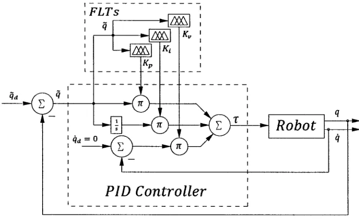
The F S T P I D Controller is an extension to the P I D Controller for non-linear sys-tems. It consists of a fuzzy system tuning online the P I D controller settings depending onzyxwvutsrqponmlkjihgfedcbaZYXWVUTSRQPONMLKJIHGFEDCBA qi and qt. Equation of this controller is expressed as:
where KzyxwvutsrqponmlkjihgfedcbaZYXWVUTSRQPONMLKJIHGFEDCBAp(q), Kt(q) and Kv(q) are 2 x 2 diagonal matrices with entries KPi(q~i), Kit(qi)
and KVi(q~i) respectively.
Figure 4.2 shows a block diagram of the F S T P I D Controller.
In order to tune the gains according to the input, a conceptual Fuzzy Logic Tuner (FLT) is defined. The conceptual F L T is composed by one input \x\ and the corre-sponding output y (see figure 4.2), which can be seen as a static mapping H defined
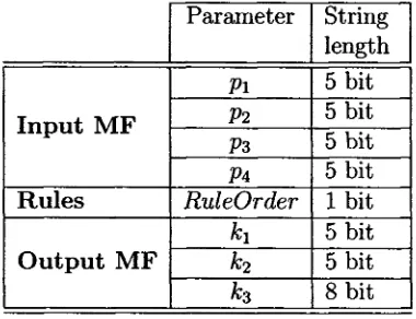
The universes of discourse of |x| and y are partitioned into three fuzzy sets: B
(Big), M (Medium) and S (Smalt) each described by a M F . Trapezoidal M F s are used for input variables and singleton M F s for output variables, this is illustrated in figure (4.3)
by
Figure 4.3: F L T parameters.
4.3. The correspondingzyxwvutsrqponmlkjihgfedcbaZYXWVUTSRQPONMLKJIHGFEDCBA Small, Medium and Big M F s for the input variable |x| are denoted by
(4.5)
For the output variable y, the corresponding singleton M F s to Small, Medium and