Effects of future climate change and habitat loss in the distribution of frog species in the Ecuadorian Andes

(1)

(2)

PONTIFICIA UNIVERSIDAD CATÓLICA DEL ECUADOR

FACULTAD DE CIENCIAS EXACTAS Y NATURALES

ESCUELA DE CIENCIAS BIOLÓGICAS

Effects of future climate change and habitat loss in the distribution of frog species in the Ecuadorian Andes

Tesis previa a la obtención del título de

Magíster en Biología de la Conservación

DAYANA GABRIELA BARRAGÁN ALTAMIRANO

(3)

Certifico que la tesis de Maestría en Biología de la Conservación de la candidata Dayana Gabriela Barragán Altamirano ha sido concluida de conformidad con las normas establecidas; por lo tanto, puede ser presentada para la calificación correspondiente.

Firma de Director de Tesis

(4)

ACKNOWLEDGEMENTS

(5)

LIST OF FIGURES

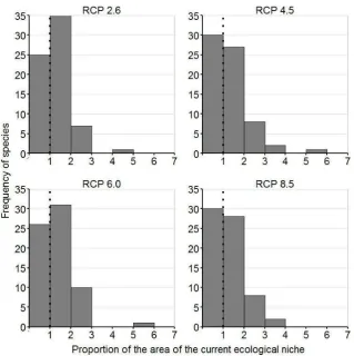
Figure 1. Frequency distribution of the proportion of change in the area of the current ecological niche of endemic frogs species in the Ecuadorian Andes by 2050. Four Representative Concentration Pathway scenarios of climate change are

shown………41

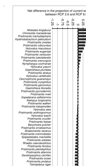
Figure 2. Net difference in the effects of Representative Concentration Pathway 2.6 and Representative Concentration Pathway 8.5 (effects of Representative Concentration Pathway 8.5 – effects of Representative Concentration Pathway 2.6) in the proportion of the area of current ecological niche of endemic frogs species in the Ecuadorian Andes by

2050. ………42

Figure 3. Proportions of change in the area of distribution of endemic frogs species of the Ecuadorian Andes by 2050. Four dispersal scenarios and four climate change models are

shown. ……….…43

Figure 4. Frequency of endemic frogs species current distribution under habitat loss in the

year 2008 in the Ecuadorian Andes………...44

Figure 5. Change in habitat loss by the year 2050 in Ecuador based on the land cover changes in the year 2000 and 2008 (Ministerio del Ambiente, 2012). ………45 Figure 6. Proportions of change in the area of current distribution of endemic frogs species of the Ecuadorian Andes by 2050. No-dispersal scenario and universal scenario under Representative Concentration Pathway 2.6 and Representative Concentration Pathway 8.5

with and without habitat loss are shown………46

(7)

climate change are shown assuming universal dispersal of the species. Dark grey represents

habitat loss extracted by 2050………47

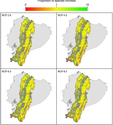
Figure 8. Change in absolute species richness of endemic frogs species in the Ecuadorian Andes by 2050. Four Representative Concentration Pathway scenarios of climate change are shown assuming universal dispersal of the species. Dark grey represents habitat loss

(8)

LIST OF TABLES

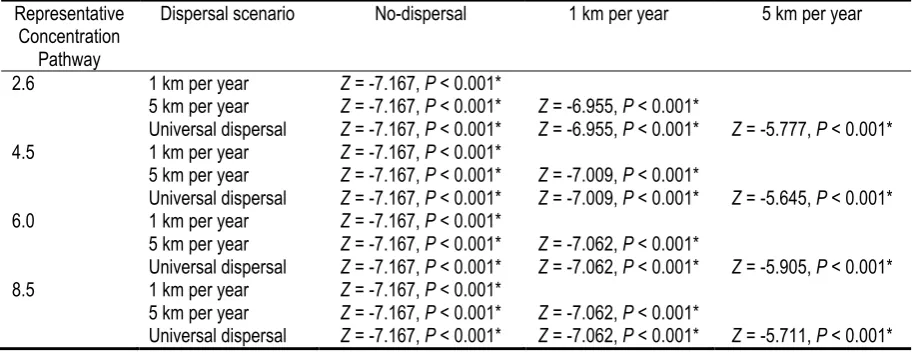
Table 1. Wilcoxon tests analysis of the proportion of change (current species distribution ÷ future ecological niche model under climate change and dispersal scenarios) in the distribution area of endemic frogs species in the Ecuadorian Andes by 2050 under

Representative Concentration Pathways and dispersal scenarios………49

Table 2. Land cover categories of the habitat loss map by the year 2050 in Ecuador and the

Ecuadorian Andes.………50

Table 3. Spearman correlations between the proportion of change in species richness of endemic frogs of the Ecuadorian Andes and bioclimatic variables under climate change and habitat loss in 2050. Samples were taken from 500 randomly generated localities

throughout the Ecuadorian Andes………51

Table 4. Spearman correlations between change in number of species of endemic frogs of the Ecuadorian Andes and bioclimatic variables under climate change and habitat loss in 2050. Samples were taken from 500 randomly generated localities throughout Ecuadorian

Andes………52

Table 5. Categories of conservation status based on the B1 criterion of the IUCN Red List (UICN, 2012) of endemic frogs species of the Ecuadorian Andes. Analysis based on current distributions and 2050 distributions according to predictions of climate change and

(9)

1. ABSTRACT

The biodiversity of the tropical Andes is threatened by climate change and habitat loss. Many studies have focused in the future effects of climate change on species distribution and conservation but few have included the effects habitat loss in their predictive studies. In this study we evaluated the combined effects of these two threats in the future distributions of endemic frogs species of the Ecuadorian Andes to the year 2050. We used ecological niche models to predict the distribution of 68 frog species using a combination of four Representative Concentration Pathway scenarios of future climate and four scenarios of dispersal capabilities. We constructed a predictive model of natural vegetation loss in Ecuador by 2050 using the Multi-Layer Perceptron neural network and Markov Chain analysis algorithms. We also explored how changes in frogs species richness resulting from climate change and habitat loss correlate with altitude and magnitude of climate change. Our results show climate change had a positive effect on the future distribution area of ~60% of the frogs species, and a negative effect in ~40%. Dispersal capabilities greatly influenced the effect of climate change and habitat loss on distribution areas. Change in species richness due to climate change show positive correlations mainly with altitude, temperature and precipitation. Future habitat loss will exacerbate the negative effects of climate change and will limit its positive effects on frogs

(10)

2. RESUMEN

La biodiversidad de los Andes tropicales está siendo amenazada por el cambio climático y

la pérdida de hábitat. Varios estudios se han enfocado en los efectos futuros del cambio climático

en la distribución de las especies pero pocos han incluido los efectos de la perdida de hábitat en sus

predicciones. En este estudio evaluamos los efectos combinados de estas dos amenazas en las

distribuciones futuras de las especies endémicas de ranas de los Andes ecuatorianos para el año

2050. Utilizamos modelos de idoneidad de hábitat para predecir la distribución de 68 especies de

ranas con una combinación de cuatro escenarios Representative Concentration Pathways de clima

futuro y cuatro escenarios de capacidad de dispersión. Hicimos un modelo predictivo de cambio de

la vegetación natural en el Ecuador para el 2050 usando los algoritmos Multi-Layer Perceptron

neural network y el análisis de cadenas de Markov. También exploramos como los cambios en la

riqueza de especies de anfibios resultantes del cambio climático y la perdida de hábitat se

correlacionan con la altura y la magnitud del cambio climático. Nuestros resultados muestran que el

cambio climático tuvo un efecto positivo en el área de distribución futura para ~ 60% de especies

de ranas, y un efecto negativo para ~ 40%. Las capacidades de dispersión influenciaron

enormemente en el efecto del cambio climático y la perdida de hábitat en las áreas de distribución.

Cambios en la riqueza de las especies muestran correlaciones positivas principalmente con la

altura, temperatura, y precipitación. La futura perdida de hábitat exacerbará los efectos negativos

del cambio climático y limitará sus efectos positivos en la distribución de las especies de anfibios.

Nuestros resultados sugieren que, bajo escenarios de dispersión limitados, la mayor parte de

anfibios de los Andes serán incapaces de colonizar efectivamente nuevos hábitats idóneos como

resultado del cambio climático y la pérdida de hábitat. En contraste, bajo escenarios de dispersión

de 5 km por año o más, el cambio climático pudiera tener un efecto beneficioso en el área de

distribución de la mayoría de especies. No existen estudios específicos sobre las capacidades de

dispersión de los anfibios en los Andes. Nuestro estudio, ilustra el rol de la dispersión en el efecto

(11)

3. INTRODUCTION

The Tropical Andes house an enormous biological richness with high levels of endemism (Gentry, 1982; Myers et al. 2000; Mittermeier et al. 2004; Killeen et al. 2007; Young and León 2007; Sarkar et al. 2008; Young, 2011). Yet, the tropical Andes are one of the most endangered biodiversity hotspots in the planet because of threats imposed by habitat loss and anthropogenic climate change (Myers et al. 2000; Mittermeier et al. 2004; Herzog et al. 2011). Habitat loss in the Andes is severe as its land cover has been

transformed into “humanized landscapes” for millennia (Rodríguez-Mahecha et al. 2004; Young, 2009; Suárez et al. 2011; Cuesta et al. 2012). Moreover, climate change in the tropical Andes has already caused changes in temperature and humidity patterns, and several studies estimate the Andes will be one of the most affected regions in the world (Bradley et al. 2006; Young, 2009; Feeley and Silman 2010; Anderson et al. 2011, Cuesta et al. 2012). Therefore, research and opportune conservation measures are vital to protect the biodiversity of the tropical Andes.

(12)

2007) have caused amphibian declines even in pristine environments of the Tropical Andes (Ron et al. 2003; Merino-Viteri et al. 2005). Moreover, the Andes hold the highest endemism of amphibian species in South America (Duellman, 1999). Andean endemic species tend to be restricted to small and specific habitats which tend to be isolated, topographically irregular, have specific key elements for survival, and climatic stable conditions (Larsen et al. 2011; Duellman, 1999). These features put Andean endemic species of frogs at an even higher risk from habitat loss and climate change.

Ecuador is the third most amphibian-diverse country in the world (Chanson et al. 2008; Ron et al. 2014), and most of the country’s endemic amphibian species occur in the

Andean montane forests (Ron et al. 2011). The Ecuadorian Andes are not exempt from habitat loss and climate change pressures. This region of Ecuador has suffered important changes in its original land cover (Sierra and Stallings 1998; Sierra, 2013) with mean annual mean deforestation ranging from 32,209 to 85,686 ha between 1990–2000 and 2000–2008 (Ministerio del Ambiente, 2012). Moreover, climate in the Ecuadorian Andes has suffered a temperature increment of approximately 0.1°Celsius per decade between 1939 and 2006 (Bradley et al., 2006; Vuille, 2008). Both habitat loss and climate change are predicted to continue their current trends in the future (Bradley et al. 2006; Vuille, 2008; Sierra, 2013). It is necessary to study the effects of climate change in amphibian climatic envelops along a parallel process of land cover change to elaborate conservation plans which allow the survival of frogs in the long-term (Mittermeier et al. 2004; Ron, 2008; Young, 2009).

(13)

(14)

4. MATERIALS AND METHODS

4.1 EFFECTS OF CLIMATE CHANGE IN SPECIES DISTRIBUTIONS

4.1.1 SPECIES SAMPLING

Our study focused on endemic species of frogs of the Ecuadorian Andes. Amphibians have been successfully used as models to study environmental changes (Hopkins, 2007). We considered endemic species because it ensures their whole distribution is included in the analyses. Ecuador is an ideal region to study the effects of climate change and habitat loss in the Andean frog biodiversity. The unique geographical features of the country have promoted high diversity and endemism (Gentry, 1982). The Ecuadorian Andes possess 165 endemic frogs, and amphibians in general have been exhaustively sampled in the country (Ron et al. 2014). In this study, we used georeferenced occurrence records from the amphibian data base collection in AmphibiaWebEcuador (www.zoologia.puce.edu.ec) which holds ~ 70,000 amphibian specimens from Ecuador. This database renders a sampling density of ~ 0.247 records per squared kilometer, which is suitable considering the MZUSP museum of the University of Sao Paulo collection (biton.uspnet.usp.br/mz/), which holds the largest amphibian collection in South America with ~140,000 specimens, and a sampling density of ~0.016 records per squared kilometer. This provides an adequate data source of both number and records of species for the present study.

(15)

more locality records were considered to increase niche model accuracy (Hernandez et al. 2006; Wisz et al. 2008). To reduce spatial auto-correlation, we removed localities less than 2 km apart from each other (Hernandez et al. 2006; Hijmans 2012; Boria et al. 2014; Radosavljevic and Anderson 2014). A total of 1,659 records and 68 endemic frogs species were included in the analyses, which represents ~41% of the endemic amphibian species of the Ecuadorian Andes described to date (Ron et al. 2014).

4.1.2 SPECIES CURRENT DISTRIBUTIONS

(16)

We constructed the models using the ENMeval package (Muscarella et al. 2014) in R software version 3.2.1 (R Core Team 2014). For model evaluation we followed Shcheglovitova and Anderson (2013) and Pearson et al. (2007). For endemic frogs species with less than 25 occurrence records, we used a jacknife k-fold cross-validation using the same number of bins as collection points. For species with more than 25 occurrence records, we used the block partitioning method, which is recommended for climate change studies (Muscarella et al. 2014). Feature class and regularization multiplier combinations were tested for model construction as recommended by Merow et al. (2013), and Radosavljevic and Anderson (2014). Models were constructed using combinations of regularization multipliers of 0.5 to 4 with 0.5 increments with feature combinations L, LQ, LP, LQH, LQP, LQHP, H, QH, HP, HQP, and LQHP (where L = linear, Q = quadratic, H = hinge, and P = product) (Muscarella et al. 2014; Radosavljevic and Anderson 2014). Combinations produced 88 models per endemic frog species. For each species we chose

the model with lowest “minimum training presence” omission rate (ORMTP) among models and with delta of Akaike’s information criterion (ΔAIC) lower than two (Burnham and

Anderson 2004; Muscarella et al. 2014; Radosavljevic and Anderson 2014).

To determine the current ecological niche model, we used as presence-absence

(17)

west of the Andes because of geographical isolation (dos Santos et al. 2015). Hence, predicted distribution in the western Andes was eliminated. Another example is Telmatobius niger whose ecological niche model predicts the species in a wide latitudinal range over the Andes. Yet, the species has only been recorded in the central Andes (Merino-Viteri et al. 2005) despite extensive sampling in the northern Andes (Ron et al. 2014). As a result, the species current ecological niche was cropped accordingly. Such analyses were applied for all species. The resulting polygons were used as estimates of the current distribution of each species.

4.1.3 SPECIES DISTRIBUTIONS UNDER CLIMATE CHANGE

For each analyzed species of endemic frogs of the Ecuadorian Andes, we projected ecological niche models using predicted climatic variables for the year 2050. The general circulation model (GCM) was HadGEM2-ES of the Met Office from the Hadley Center (HadGEM2 Development Team, 2011) as it is considered stable and realistic (Collins et al. 2011; Jones et al. 2011; HadGEM2 Development Team et al. 2011), and performs well in the tropics (Martin et al. 2011). HadGEM2-ES was evaluated using Representative Concentration Pathways (RCPs) which are a new generation of climate scenarios which incorporate the latest economic, technological, and environmental global information to represent future climate conditions (Moss et al. 2010b; Jones et al. 2011). RCPs were selected as the best models in the Coupled Model Intercomparison Project 5 (Jones et al. 2011) and were released for the Fifth Assessment Report of the Intergovernmental Panel on Climate Change (Collins et al. 2011; Jones et al. 2011).

(18)

current ecological niche model. Future climatic variables were the same as those selected

for the current ecological niche models. The “maximum training plus specificity” threshold

was applied to the projected niche models, and the resulting polygon was considered as the geographic distribution in year 2050.

Projected niche models for future climate change were cut according to four dispersal scenarios. Scenarios included: no-dispersal, 1 km per year, 5 km per year, and universal dispersal. These scenarios were selected based on expert criteria and the literature (reviewed in Wells, 2007). The maximum dispersal distance recorded for an amphibian is 55 km per year (Rhinella marina, B. L. Phillips et al. 2007) and was originally considered as a dispersal scenario; but, was eliminated as it did not differentiated from the universal dispersal scenario when applied to the analyzed distributions of frogs. The 1 km and 5 km dispersal scenarios were calculated as the Euclidean distance from the limits of the current distribution to the closet suitable area in the future scenario using the software R (R Core Team, 2015). Under the universal-dispersal scenario the future ecological niche model was not cut. The other scenarios restricted the future ecological niche model depending on the scenario of the distance covered per year. Resulting polygons were assumed as scenarios of future distributions for each endemic frogs species of the Ecuadorian Andes.

(19)

universal dispersal scenarios because they show the pure effect of climate change under all RCP scenarios. Also, we compared proportions between dispersal scenarios under all RCP scenarios using Wilcoxon tests.

4.2 EFFECTS OF CLIMATE CHANGE AND HABITAT LOSS IN SPECIES

DISTRIBUTIONS

4.2.1 PREDICTIVE MODEL OF HABITAT LOSS

We modeled future habitat loss for the year 2050 for mainland Ecuador using the Land Change Modeler for Ecological Sustainability (Eastman, 2012) as implemented in the software IDRISI Selva v17.02 (Clark Labs, Worcester, MA, USA). This modeling strategy has high performance to predict land cover change (Mas et al. 2014). To construct the model, we identified historic trends of habitat loss driven by predictor variables, validated these trends, and extrapolated them to predict future habitat loss (Clark Labs, 2009; Eastman, 2012). We constructed separated models for Coast, Andean, and Amazonian regions of Ecuador because their driving factors for habitat loss are different (Sierra, 2013). We followed Peralvo and Delgado (2010) geographical limits of the Ecuadorian regions. Besides, geographical partitioning is suggested to increase model transparency (Robinson, 2008). We constructed the models based on maps of habitat loss of Ecuador for the years 1990, 2000, and 2008 (Ministerio del Ambiente, 2012). Habitat loss maps had two habitat categories: presence of natural vegetation (e.g. native forest, shrubs, and herbaceous vegetation; Ministerio del Ambiente 2012b) and absence of natural vegetation (e.g. crops, pasture, urban areas, water, and glaciers). Historical changes in land cover were measured by identifying changes in categories between 1990 and 2000 (Eastman et al. 2005).

(20)

altitude, slope, proximity to roads, proximity to settlements, proximity to rivers, proximity to disturbance, population density, and agricultural suitability. See Appendix 1 for details

on data source and preparation of predictor variables. We tested the level of association between variables and land cover transitions using Cramer’s V analysis; variables with coefficients under 0.15 were eliminated from the model (Eastman, 2012). We calculated transition potential maps based on the interaction of the predictor variables and the gain and loss of natural habitat (Eastman, 2012). Transition potential maps show the susceptibility of habitat categories to change between each other as the effect of predictor variables (Eastman, 2012). Estimates were based on the Multi-Layer Perceptron (MLP) method of neural networks (Bishop, 1995; Lek and Guégan, 1999). This method’s products have been shown as highly accurate when modeling predictive land cover change (Pérez-Vega et al. 2012). MLP calculations were based on 10,000 pixels half of which were used for testing and half for training, over 10,000 interactions. Modelling parameters were set to default values as recommended by Eastman (2012).

(21)

land cover scenario was resampled to a 30 arc-second resolution (i.e. ~1 km2) using the Nearest Neighbor resampling method as the best option for categorical data (Parker et al. 1983).

4.2.2 SPECIES DISTRIBUTIONS UNDER CLIMATE CHANGE AND HABITAT LOSS We estimated the current species distributions under habitat loss by removing all the areas with absence of natural vegetation in 2008 from the species current distribution. We also removed water body areas because none of our modeled species are aquatic. To obtain the species distributions under climate change and habitat loss in 2050, we calculated new dispersal scenarios from the current species distributions under habitat loss; then, we removed all the areas with absence of natural vegetation in the 2050 per dispersal scenario. Then, we calculated the proportion of change in area of species distribution under habitat loss for each dispersal scenario. We obtained the proportions by dividing the distribution area under climate change and habitat loss in 2050 by the current distribution areas.

(22)

4.3 SPATIAL PATTERNS IN THE EFFECT OF CLIMATE CHANGE UNDER

HABITAT LOSS IN SPECIES DISTRIBUTIONS

The current distributions of all endemic frogs species were added into a single map to generate a map of species richness. The same map was generated for future distributions under each RCP scenario under the universal-dispersal scenario. Future maps of species richness were divided by the current map of species richness to obtain maps showing the proportion of change in species richness. Future maps of species richness were also subtracted from the current map to obtain maps showing the change in absolute species richness. Similarly, we calculated the proportion of change between current climate and the 2050 climate for annual mean temperature (bio1), maximum temperature of warmest month (bio 5), minimum temperature of coldest month (bio 6), annual precipitation (bio 12), and precipitation of driest month (bio 14) for each RCP scenario. Elevation data (SRTM; Ferr et al. 2007) was also considered for the spatial pattern analysis. Spatial resolution of the elevation data was resampled from its original 90 m. into the spatial resolution of the climatic variables used for the ecological niche modeling (~1km2). We removed the habitat loss in 2050 from the maps of proportion of change in species richness, change in absolute species richness, proportion of change in climate, and the elevation. All maps and operations were performed using the Raster package (Hijmans, 2015) in the software R (R Core Team, 2015).

We obtained a matrix with the values per pixel of the proportion of change in species richness, the change in absolute species richness, the proportion of change between current and 2050 climate, and elevation with the software ArcGIS 10.2 ESRI (Redlands CA, USA). Then, we tested the correlation between the extracted values of the maps with

(23)

random sample of 500 pixels. All correlation analyses were performed using Hmisc package (Harrell, 2015) in the software R (R Core Team 2015).

4.4 CHANGES IN CONSERVATION STATUS AS A RESULT OF CLIMATE

CHANGE AND HABITAT LOSS IN 2050

(24)

5. RESULTS

Under the universal dispersal scenario, climate change caused an average 60% of endemic frogs species of the Ecuadorian Andes to increase their area of ecological niche (Figure 1). The effects of climate change were significantly different only between RCP scenarios 2.6 and 8.5, where RCP 8.5 showed smaller proportions of the current ecological niche of species compared to RCP 2.6 (Z = -3.074, P = 0.002) (Figure 2). On the other hand, dispersal scenarios showed significant differences in the proportion of change in the area of distribution under all RCP scenarios (Figure 3, Table 1).

DITRIBUTIONS

Selected predictor variables to model the habitat loss in the year 2050 were specific in Coastal, Andean, and Amazonian Ecuador and are summarized in Appendix 1. The validations of predicted models in 2008 per region were accepted, showing the following results: Coast AUC = 0.904; Andes AUC = 0.926, Amazonia AUC = 0.858.

(25)

The combined effects of climate change and habitat loss on frogs species are highly dependent on the dispersal scenario. Under a non-dispersal scenario, average proportion of change in distribution range is 0.379 ± 0.162 of the current distribution; under a 1 km dispersal it is 0.674 ± 0.318; under a 5 km dispersal it is 0.970 ± 0.872; and, under universal dispersal scenario, average proportion of change in distribution range is 1.03 ± 0.935 (Figure 6).

The proportion of change in species richness of endemic frogs of the Ecuadorian Andes in 2050 under climate change increased with mean annual temperature and precipitation of the driest month under all RCP scenarios (Table 3). Altitude and maximum temperature of the warmest month were also associated with increase in species richness proportion under the scenarios RCP 2.6, RCP 4.5, and RCP 6.0, and annual precipitation under the scenarios RCP 2.6 and RCP 8.5. Spatial pattern of proportion of change in species richness with habitat loss in 2050 is shown in Figure 7.

(26)

5.4 CHANGES IN CONSERVATION STATUS AS A RESULT OF CLIMATE

(27)

6. DISCUSION

DITRIBUTIONS

Many studies have addressed the effects of climate change in future species distributions (e.g. Peterson et al., 2002 ; Araújo et al., 2006; Lawler et al., 2009; Freeman et al., 2013) and the effects of habitat loss in biodiversity (e.g. Brooks et al., 2002; Sangermano, et al., 2012; Estavillo et al., 2013). However, none of them have considered the effect of both threats simultaneously, and therefore provide a partial view of the conservation future of species. In this study we combined scenarios of climate change and habitat loss to provide more reliable predictions of the conservation future of species. This integrative approach should better guide conservation efforts to ameliorate the effects of climate change and habitat loss.

Our results showed that the effect of climate change will potentially benefit the majority of frogs species while future change in natural vegetation cover varies with location but has an overall negative effect. Climate change could benefit ~60% of the analyzed species by potentially increasing their area of distribution 65%. However, the combined effects of climate change and habitat loss will limit the potential gain of distribution area to ~3%.

(28)

depends on the dispersal abilities of each species (Cushman, 2006). As a result, dispersal will strongly influence the ability of frogs to follow shifts in their climate envelope and colonize new areas of regenerated habitat. Dispersal will allow species whose distributions are reduced by climate change and habitat loss to atenuate such negative effect, and species whose distribution areas are increased by these phenomena to seize the oportunity to colonize new areas.

At present, there are no studies showing the dispersal capabilities of Andean frogs. This limits our hability to identify the most probable dispersal scenario in our study based on factual data. In our study dispersal scenarios were based on Euclidean distances. We did not considered topographic barriers, climatic barriers, and habitat fragmentation, which are important factors limiting dispersal. Distance measurements considering topography do not differ significantly from Euclidean distance (G. Galarza, personal communication). Yet, barriers related to fragmentation (e.g. cities, roads, farmland) should exert great limitations on the ability of Andean frogs to disperse (Cushman, 2006). In general, frogs do not tend to migrate as much as other vertebrates (Wells, 2007). Hence, dispersal under climate change and habitat loss might be more closely reflected by our limited dispersal scenarios.

(29)

active species to be more vulnerable to climate change and habitat loss (Bowler and Benton, 2005). Studies of dispersal capabilities of specific frog species of the Andes should further elucidate this matter. As a result, despite the general trend in amphibians is to show reduced dispersal, studies show amphibian species could show great dispersal capabilities under the right ecological circumstances. It is crucial to perform specific studies on

Andean frog’s dispersal capabilities that could elucidate their aptitude to cope with climate change and habitat loss.

It has been stated that climate change will cause mountain species to follow suitable climate by migrating uphill, fleeing from warming climate (Walther et al. 2002; Parmesan, 2006; Colwell et al. 2008; Sekercioglu et al. 2008; Lawler et al. 2009; Feeley and Silman 2010). Our results suggest that the proportion of change in species richness and absolute change in species richness will increase with altitude. This suggests endemic frog species in the Ecuadorian Andes will respond as expected and tend to migrate uphill. Proportion of change of species richness increased in areas with increased mean annual temperature and precipitation on the driest month. This concurs with the physiological preference of amphibians for warm environments due to ecotothermality, and preference for wet areas because of their sensitiveness to dissecation (Wells, 2007).

(30)

probably responds to the high spatial heterogeneity of the Andean climate (Gentry, 1982; Killeen et al. 2007; Young and León 2007). Such effects of climate change have been shown to be complex (Garcia et al. 2014). Other metrics of evaluation on specific regions could further elucidate the nature of the effect of climate change in spatial shifting of species climate envelopes (e.g. specific gain and loss of species, orientation on envelope shifting) (Garcia et al. 2014; Cuesta et al., 2015).

RCPs were designed to represent scenarios of climate change that increase in intensity from the RCP 2.6 (i.e. the less drastic scenario) to the RCP 8.5 (i.e. the most drastic scenario) (Moss et al. 2010a; Vuuren et al. 2011). Therefore, RCPs 2.6 and 8.5 are the most differentiated climate change scenarios. Accordingly, our results showed difference in the effects of climate change only between RCP scenarios 2.6 and 8.5. The effects of RCP 8.5 showed smaller proportions of the original ecological niche for the majority of species compared to the effects of RCP 2.6. This suggests that more drastic climate change scenarios tend to limit ecological niche expansion for the species that were positively affected by climate change, and further reduce ecological niche area for the species that were negatively affected.

6.4 CHANGES IN CONSERVATION STATUS AS RESULT OF CLIMATE

(31)

(32)

7. LITERATURE CITED

Alford, R. A., Bradfield, K. S., Richards, S. J. 2007. Ecology: global warming and amphibian losses. Nature (7144): E3–E4.

Araújo, M. B., Thuiller, W., Pearson R. G. 2006. Climate warming and the decline of amphibians and reptiles in Europe. Journal of Biogeography (10): 1712–1728.

Anderson, E. P., Marengo, J., Villalba, R., Halloy, S., Young, B., Cordero, D., Gast, F., Jaimes, E., Ruiz, D. 2011. Consequences of climate change for ecosystems and ecosystem services in the Tropical Andes. In: Climate change and biodiversity in the tropical andes (S. K. Herzog, R. Martínez, P. M. Jørgensen, H. Tiessen, eds) pp. 1–18. Inter-American Institute for Global Change Research (IAI) and Scientific Committee on Problems of the Environment (SCOPE), Paris.

Bishop, C. M. 1995. Neural networks for pattern recognition. Oxford University Press, Oxford.

Boria, R. A., Olson, L. E., Goodman, S. M., Anderson, R. P. 2014. Spatial filtering to reduce sampling bias can improve the performance of ecological niche models. Ecological Modelling 275: 73–77.

Bowler, D. E., Benton, T. G. 2005. Couses and consecuences of animal dispersal strategies: relating individual behavior to spatial dinamics. Biological reviews 80: 205–225.

Brooks, T. M., Mittermeier, R. A., Mittermeier, C. G., Fonseca, G. A., Rylands, A. B., Konstant, W. R., Hilton-taylor, C. 2002. Habitat loss and extinction in the hotspots of biodiversity. Conservation Biology(4): 909–923.

Burnham, K. P., Anderson, D. R. 2004. multimodel inference: understanding AIC and BIC in model selection. Sociological Methods y Research (2): 261–304.

Burnham, B.O. 1973. Markov intertemporal land use simulation model. Southern Journal of Agricultural Economics (1): 253–258.

Bradley, R. S., Vuille, M., Diaz, H. F., Vergara, W. 2006. Threats to water supplies in the Tropical Andes. Science (5781): 1755–1756.

Chanson, J., Hoffmann, M., Cox, N., Stuart, S. 2008. The state of the world’s amphibians.

En: Threatened Amphibians of the World (S.N. Stuart, M. Hoffmann, J.S. Chanson, N.A. Cox, R.J. Berridge, P. Ramani, B.E Young, eds) pp. 33–54. Lynx Ediciones, Barcelona.

(33)

Collins, W. J., Bellouin, N., Doutriaux-Boucher, M., Gedney, N., Halloran, P., Hinton, T., Hughes, J. et al. 2011. Development and evaluation of an earth-system model – HadGEM2. Geoscientific Model Development 4: 1051–1075.

Coloma, L. A., Frenkel, C. Ortiz, D. A. 2012. Hyloxalus jacobuspetersi. En: Ron, S. R., Guayasamin, J. M., Yanez-Muñoz, M. H., Merino-Viteri, A., Ortiz, D. A. y Nicolalde, D. A. 2014. AmphibiaWebEcuador. Version 2014.0. Museo de Zoología, Pontificia Universidad Católica del Ecuador.

<http://zoologia.puce.edu.ec/vertebrados/anfibios/FichaEspecie.aspx?Id=1239>, acceso noviembre 01, 2015.

Colwell, R. K., Brehm, G. Cardelús C. L., Gilman, A. C., Longino, J. T. 2008. Global warming, elevational range shifts, and lowland biotic attrition in the wet tropics. Science (5899): 258–261.

Corn, P. S. 2005. Climate change and amphibians. Animal Biodiversity and Conservation (1): 59–67.

Cuesta, F., Merino-Viteri, A., Muriel, P., Baquero, F., Freile, J., Torres, O., Peralvo, M. 2015. Escenarios de impacto del cambio climático sobre la biodiversidad del Ecuador continental y sus implicaciones en el sistema nacional de áreas protegidas. Ministerio del Ambiente del Ecuador. CONDESAN. Escuela de Ciencias Biológicas, Pontificia Universidad Católica del Ecuador, Quito.

Cuesta, F., Bustamante, M., Becerra, M. T., Maldonado, G. 2012. Introducción: cambio climático y los Andes Tropicales. En: panorama andino de cambio climático: vulnerabilidad y adaptación en los Andes Tropicales (F. Cuesta, M. Bustamante, M.T. Becerra, J. Postigo, J. Peralvo, eds) pp. 13–17.CONDESAN, SGCAN, Lima.

Cushman, S. A. 2006. Effects of habitat loss and fragmentation on amphibians: a review and prospectus. Biological Conservation (128): 231–240.

Danielsson, P-E. 1980. Euclidean distance mapping. Computer Graphics and Image Processing (3): 227–48.

dos Santos, S. P., Ibáñez, R., Ron, S. R. 2015. Systematics of the Rhinella margaritifera complex (Anura, Bufonidae) from western Ecuador and Panama with insights in the biogeography of Rhinella alata. ZooKeys 501:109-145.

Duellman, W. E. 1999. Distribution patterns of amphibians in South America. En: Patterns of distributions of amphibians: a global perspective, pp. 255–328. John Hopkins University Press, Baltimore.

Earth Observation Group. DMSP-OLS nighttime lights time series. 1992. Version 4. Resolution 30 arc-seconds. National Center for Environmental Information.

(34)

Eastman, J. R., Solorzano, L. A., Van Fossen, M. 2005. Transition potential modeling for land-cover change. In: Maguire DJ, Batty M, Goodchild MF. GIS, spatial analysis and modeling. ESRI Press, Redlands.

Elith, J., Graham, C. H., Anderson, R. P., Dudík, M., Ferrier, S., Guisan, A., Hijmans, R. J., Huettmann, F., Leathwick, J. R., Lehmann, A., Jin, L., Lohmann, L. G., Loiselle, B. A., Manion, G., Moritz, C., Nakamura, M., Nakazawa, Y., McC. J., Overton, A. Peterson, T., Phillips, S. J., Richardson, K., Scachetti-Pereira, R., Schapire, R. E., Soberón, J., Williams, S., Wisz, M. S., Zimmermannet N. E. 2006. Novel methods

improve prediction of species’ distributions from occurrence data. Ecography (29): 129–151.

Estavillo, C., Pardini, R., da Rocha, P. L. B. 2013. Forest loss and the biodiversity threshold: an evaluation considering species habitat requirements and the use of matrix habitats. PloS One (12): e82369.

Farr, T. G., Rosen, P. A., Caro, E., Crippen, R. 2007. The shuttle radar topography mission. Reviews of Geophysics (45):1–33.

Feeley, K. J., Silman, M. R. 2010. Land-use and climate change effects on population size and extinction risk of Andean plants. Global Change Biology (12): 3215–3222. Freeman, L. A, Kleypas, J. A, Miller, A. J. 2013. Coral reef habitat response to climate

change scenarios. PloS One (12): e82404.

Garcia, R. A., Cabeza, M. Rahbek, C. Araújo, M. B. 2014. Multiple dimensions of climate change and their implications for biodiversity. Science (6183): 1247579.

Gentry, A. H. 1982. Neotropical floristic diversity: phytogeographical connections between central and south America, pleistocene climatic fluctuations, or an accident of the Andean orogeny? Annals of the Missouri Botanical Garden (69): 557–593.

Harrell, F. E. 2015. Hmisc: Harrell Miscellaneous. R package version 3.16–0. http://CRAN.R-project.org/package=Hmisc.

Hernandez, P. A., Graham, C. H., Master, L. L., Albert, D. L., The, A. D. L. 2006. The effect of sample size and species characteristics on performance of different species distribution modeling methods. Ecography (29): 773–785.

Herzog, S. K., Martínez, R., Jørgensen, P. M., Tiessen, H. 2011. Climate change and biodiversity in the Tropical Andes. Inter-American Institute for Global Change Research (IAI) and Scientific Committee on Problems of the Environment (SCOPE), Paris.

Hijmans, R. J. 2015. Raster: geographic data analysis and modeling. R package version 2.4-15. http://CRAN.R-project.org/package=raster.

(35)

Hijmans, R. J., Cameron, S.E., Parra, J. L., Jones, P. G., Jarvis, A. 2005. Very high resolution interpolated climate surfaces for global land areas. International Journal of Climatology (25): 1965–1978.

Hopkins, W. A. 2007. Amphibians as models for studying environmental change. ILAR Journal (3): 270–7.

Instituto Ecuatoriano de Estadísticas y Censos. 2010. Cartografía digital 2010. Cartografía censal.

IUCN. 2012. IUCN Red List categories and criteria. Version 3.1.

Jones, C. D., Hughes, J. K., Bellouin, N., Hardiman, S. C., Jones, G. S., Knight, J., Liddicoat, S., O Connor F. M., Institut Pierre-simon Laplace. 2011. Model development the HadGEM2-ES implementation of CMIP5 centennial simulations. Geoscientific Model Development (4) 543–570.

Killeen, T. J., Douglas, M., Consiglio, T., Jørgensen, P. M., Mejia, J. 2007. Dry spots and wet spots in the Andean hotspot. Journal of Biogeography (8): 1357–1373.

Larrea, C. 1999. El INFOPLAN : Un Sistema de Información Para El Desarrollo Local En

El Ecuador. http://www.cepal.org/deype/mecovi/docs/TALLER6/7.pdf

Larsen, T. H., Brehm, G., Navarrete, H., Franco, P., Gomez, H., Mena, J. L., Morales, V., Argollo, J., Blacutt, L., Canhos, V. 2011. Phenology and interspecific ecological interactions of Andean biota in the face of climate change. En: climate change and biodiversity in the Tropical Andes (S. K. Herzog, R. Martínez, P. M. Jørgensen, H. Tiessen, eds) pp. 47-66. Inter-American Institute for Global Change Research (IAI) and Scientific Committee on Problems of the Environment (SCOPE), Paris.

Lawler, J. J., Shafer, S. L., White, D., Kareiva, P., Maurer, E. P., Blaustein, A. R., Bartlein, P. J. 2009. Projected climate-induced faunal change in the Western Hemisphere. Ecology (3): 588–597.

Lek, S., Guégan, J. F. 1999. Artificial neural networks as a tool in ecological modelling , an introduction. Ecological Modelling (120): 65–73.

Liu, C., White, M., Newell, G. 2013. Selecting thresholds for the prediction of species occurrence with presence-only data. Journal of Biogeography (40): 778–89.

Liu, C., Berry, P. M., Dawson, T. P., Pearson, R. G. 2005. Selecting thresholds of occurrence in the pre-diction of species distributions. Ecography (28): 385–393. Martin, G. M., Milton, S. F., Senior, C. A., Brooks, M. E., Ineson, S. 2010. Analysis and

reduction of systematic errors through a seamless approach to modeling weather and climate. American Meteorological Society (23): 5933–5957.

(36)

Merino-Viteri, A., Coloma, L. A., Almendáriz, A. 2005. Estudios sobre las ranas andinas de los géneros Telmatobius y Batrachophrynus (Anura: Leptodactylidae). Monografías de Herpetología (7): 9–37.

Merow, C., Smith, M. J., Silander, J. A. 2013. A practical guide to MaxEnt for modeling

species’ distributions : what it does, and why inputs and settings matter. Ecography (36): 1058–1069.

Ministerio del Ambiente. 2014. Patrimonio de áreas protegidas del Estado. Escala 1: 250.000. Ecuador.

Ministerio del Ambiente. 2012. Línea base de deforestación del ecuador continental, Quito, Ecuador.

Ministerio del Ambiente. 2012b. Metodología para la representación cartográfica de los ecosistemas del Ecuador continental, Quito, Ecuador.

Ministerio de Agricultura, Ganadería y Pesca. 2002. Escala 1: 250.000. WGS84 UTM zona 17 sur. Ecuador.

Ministerio de Transporte y Obras Públicas. 2013a. Red Vial Estatal. WGS84 UTM zona 17 sur.

Ministerio de Transporte y Obras Públicas. 2013b. Plan estratégico de movilidad 2020, 2028, 2037.

Mittermeier, R. A., Robles Gil, P., Hoffman, M., Pilgrim, J., Brooks, T., Mittermeier, C. G., Lamoreux, J., da Fonseca, G. A. B. 2004. Hotspots revisited. CEMEX, Mexico DF.

Moss, R. H., Edmonds, J. A., Hibbard, K. A., Manning, M. R., Rose, D.K., van Vuuren, D. P., Carter, T. R., Emori, S., Kainuma, M., Kram, T., Meehl, G. A., Mitchell, J. F. B., Nakicenovic, N., Riahi, K., Smith, S. J., Stouffer, R. J., Thomson, A. M., Weyan, J.P., Wilbanks, T. J. 2010. The next generation of scenarios for climate change research and assessment. Nature (7282): 747–756.

Moss, R., Babiker, M., Brinkman, S., Calvo, E., Carter, T., Edmonds, J., Elgizouli, I., Emori, S., Erda, Lin., Hibbard, K., Jones, R., Kainuma, M., Kelleher, J., Lamarque, J. F. Manning, M., Matthews, B., Meehl, J., Meyer, L., Mitchell, J., Nakicenovic, N.,

O’Neill, B., Pichs, R., Riahi, K., Rose, S., Runci, P., Stouffer, R., van Vuuren, D.,

Weyant, J., Wilbanks, T., van Ypersele, J. P., Zurek, M. 2008. Towards new scenarios for analysis of emissions, climate change, impacts, and response strategies. Intergovernmental Panel on Climate Change, Geneva.

(37)

Myers, N., Mittermeier, R. A., Mittermeier, C. G., da Fonseca, G. A. B., Kent, J. 2000. Biodiversity hotspots for conservation priorities. Nature 403(6772): 853–858.

Ortega-Andrade, H. M., Rojas-Soto, O., Paucar, C. 2013. Novel data on the ecology of Cochranella mache (Anura: Centrolenidae) and the importance of protected areas for this critically endangered glassfrog in the neotropics. PloS One (12): e81837.

Páez-Vacas, M. I., Coloma, L. A., Santos, J. C. 2010. Systematics of the Hyloxalus bocagei complex (Anura: Dendrobatidae), description of two new cryptic species, and recognition of H. maculosus. Zootaxa 2711:175.

Parker, J., Kenyon, R. V., Troxel, D. E. 1983. Comparison of interpolating methods for image resampling. IEEE Transactions on Medical Imaging (1): 31–39.

Parmesan, C. 2006. Ecological and evolutionary responses to recent climate change. Annual Review of Ecology, Evolution, and Systematics 37: 637–669.

Pearson, R., Raxworthy, G., Nakamura, C. J. M., Peterson, A. T. 2007. Predicting species

distributions from small numbers of occurrence records : a test case using cryptic

geckos in Madagascar. Journal of Biogeography (34):102–117.

Peralvo, M., Delgado, J. 2010. Protocolo metodológico para la generación del mapa de deforestación histórica en el Ecuador continental. Ministerio Del Ambiente Del Ecuador. http://sociobosque.ambiente.gob.ec/files/Folleto linea3.pdf.

Pérez-Vega, A., Mas, J.-F., Ligmann-Zielinska, A. 2012. Comparing two approaches to land use/cover change modeling and their implications for the assessment of biodiversity loss in a deciduous tropical forest. Environmental Modelling y Software, (1), 11–23.

Peterson, a T., Ortega-Huerta, M. a, Bartley, J., Sánchez-Cordero, V., Soberón, J., Buddemeier, R. H., Stockwell, D. R. B. 2002. Future projections for Mexican faunas under global climate change scenarios. Nature (6881): 626–629.

Phillips, B. L., Brown, G. P., Greenlees, M., Webb, J. K., Shine, R. 2007. Rapid expansion of the cane toad (Bufo Marinus) invasion front in tropical Australia. Austral Ecology (2): 169–176.

Phillips, S. J., Anderson, R. P., Schapire, R. E. 2006. Maximum entropy modeling of species geographic distributions. Ecological Modelling (3-4): 231–259.

Pounds, J. A., Bustamante, M. R., Coloma, L. A., Consuegra, J. A., Fogden, M. P. L., Foster, P. N., La Marca, E., Masters, K. L., Merino-Viteri, A., Puschendorf, R., Ron, S. R., Sánchez-Azofeifa, G. A., Still, C. J., Young, B. E. 2006. Widespread amphibian extinctions from epidemic disease driven by global warming. Nature (7073): 161–

167.

(38)

Para Aplicaciones Agropecuarias En El Ordenamiento de Territorio Y Manejo Integral de Cuencas.

PROMSA, Universidad del Azuay, Instituto de Estudios de Régimen Seccional del Ecuador, Universidad Nacional de Loja, Alianza Jatun Sacha-CDC. 2001b. Hodrografía. Ríos simples. Escala 1: 250.000. En: Sistemas de Información Geográfica Para Aplicaciones Agropecuarias En El Ordenamiento de Territorio Y Manejo Integral de Cuencas.

PROMSA, Universidad del Azuay, Instituto de Estudios de Régimen Seccional del Ecuador, Universidad Nacional de Loja, Alianza Jatun Sacha-CDC. 2001c. Uso de Suelo. Sistema Nacional de Áreas Protegidas. Escala 1: 250.000. En: Sistemas de Información Geográfica Para Aplicaciones Agropecuarias En El Ordenamiento de Territorio Y Manejo Integral de Cuencas.

PROMSA, Universidad del Azuay, Instituto de Estudios de Régimen Seccional del Ecuador, Universidad Nacional de Loja, Alianza Jatun Sacha-CDC. 2001d. Vias Y Accesos. Vías. Escala 1: 250.000. En: Sistemas de Información Geográfica Para Aplicaciones Agropecuarias En El Ordenamiento de Territorio Y Manejo Integral de Cuencas.

R Core Team. 2015. R: A language and environment for statistical computing. R Foundation for Statistical Computing, Vienna, Austria. http://www.R-project.org/. Radosavljevic, A., Anderson, R. P. 2014. Making better Maxent models of species

distributions: complexity, overfitting and evaluation. Journal of Biogeography (4): 629–643.

Rodríguez-Mahecha, J. V., Salaman, P., Jørgensen, P., Consiglio, T., Forno, E., Telesca, A., Suárez, L., Arjona, F., Rojas, F., Bensted-Smith, R., Inchausty, V. H. 2004. Tropical Andes. En: Hotspots revisited (R.A. Mittermeier, P. Robles Gil, M. Hoffman, J. Pilgrim, T. Brooks, C.G. Mittermeier, J. Lamoreux, G.A.B. da Fonseca, eds) pp. 73–79. CEMEX, Ciudad de México.

Ramirez, J., Jarvis, A. 2008. High resolution statistically downscaled future climate surfaces. International Center for Tropical Agriculture (CIAT); CGIAR Research Program on Climate Change, Agriculture and Food Security (CCAFS), Cali.

Robinson, S. 2008. Conceptual modelling for simulation part I: definition and requirements. Journal of the Operational Research Society (59): 278–90.

Ron, S. R., Guayasamin, J. M., Yanez-Muñoz, M. H., Merino-Viteri, A. y Ortiz, D. A. 2014. AmphibiaWebEcuador (en línea). Version 2014.0. Museo de Zoología,

Pontificia Universidad Católica del Ecuador. <

http://zoologia.puce.edu.ec/Vertebrados/anfibios/AnfibiosEcuador>, acceso 3 de enero, 2014.

(39)

Ron, S. R. 2008. Climate change. En: The amphibian extinction crisis: a call to action. Letters to the editor (K. C. Zippel, J. R. Mendelson III, eds) pp. 25–26. Herpetological Review (1): 23–29.

Ron, S. R., Duelman, W. E., Coloma, L. A., Bustamante, M. R. 2003. Population decline of the jambato toad Atelopus ignescens (Anura: Bufonidae) in the Andes of Ecuador. Journal of Herpetology (1): 116–126.

Sangermano, F., Toledano, J., Eastman, R. 2012. Land cover change in the Bolivian Amazon and its implications for REDD+ and endemic biodiversity. Landscape Ecology (4): 571–584.

Sarkar, S., Sánchez-Cordero, V., Londoño, M. C., Fuller, T. 2008. Systematic conservation assessment for the Mesoamerica, Chocó, and Tropical Andes biodiversity hotspots: a preliminary analysis. Biodiversity and Conservation (7): 1793–1828.

Sekercioglu, C. H., Schneider, S. H., Fay, J. P., Loarie, S. R. 2008. Climate change, elevational range shifts, and bird extinctions. Conservation Biology (22): 140–150. Shcheglovitova, M., Anderson, R. P. 2013. estimating optimal complexity for ecological

niche models: a jackknife approach for species with small sample sizes. Ecological Modelling (269): 9–17.

Sierra, R. 2013. Patrones y factores de deforestación en el ecuador continental, 1990-2010: Y un Acercamiento a los Próximos 10 años. Conservación Internacional Ecuador y Forest Trends, Quito.

Sierra, R., Stallings, J. 1998. The dynamics and social organization of tropical deforestation in Northwest Ecuador 1983-1995. Human Ecology (1): 135–160.

Spieler, M., Linsenmair, K. E. 1998. Migration patterns and diurnal use of shelter in a ranid frog of a West African savannah: a telemetric study. Amphibia-Reptilia 19:43– 64.

Suárez, C. F., Naranjo, L.G., Espinosa, J.C., Sabogal, J. 2011. Land use changes and their synergies with climate change. En: Climate change and biodiversity in the Tropical Andes (S. K. Herzog, R. Martínez, P. M. Jørgensen, H. Tiessen, eds) pp. 141–151. Inter-American Institute for Global Change Research (IAI) and Scientific Committee on Problems of the Environment (SCOPE), Paris.

Stuart, S. N., Hoffmann, M., Chanson, J. S., Cox, N. A., Berridge, R. J., Ramani, P., Young, B. E. 2008. Threatened amphibians of the world. IUCN, Gland, Switzerland; and Conservation International and Lynx Editions, Virginia.

(40)

Swets, J. A. 1986. Form of empirical ROCs in discrimination and diagnostic tasks: implications for theory and measurement of performance. Psychological Bulletin (2):181–198.

Tewksbury, J. J., Huey, R. B., Deutsch, C. A. 2008. Putting the heat on tropical animals. Science (320): 1296–1297.

Tunner, H. G., Kárpatí, L. 1997. The water frogs (Rana esculenta complex) of the Neusiedlersee region (Austria, Hungary). Herpetozoa (3-4): 139–148.

Twitty, V. C., Grant, D., Anderson, O. 1964. Long distance homing in the newt Taricha rivularis. Proc. Natl. Acad. Sci. 51:51–58.

Vuille, M., Francou, B., Wagnon, P., Juen, I., Kaser, G., Mark, B. G., Bradley, R. S. 2008. Climate change and tropical Andean glaciers: Past, present and future. Earth-Science Reviews (3-4): 79–96.

Vuuren, D. P., Edmonds, J. A., Kainuma, M., Riahi, K., Weyant, J. 2011. A special issue on the RCPs. Climatic Change 109 (1-2): 1–4.

Wells, K. D. 2007. The ecology and the behavior of amphibians. The University of Chicago Press, chapter 6. Chicago and London.

Young, B. E., Stuart, S. N., Chanson, J. S., Cox, N. A., Boucher, T. M. 2004. Disappearing jewels: the status of new world amphibians. NatureServe. Arlington.

Young, K. R. 2011. Introduction to Andean geographies. En: climate change and biodiversity in the Tropical Andes (S. K. Herzog, R. Martínez, P. M. Jørgensen, H. Tiessen, eds) pp. 128-140. Inter-American Institute for Global Change Research (IAI) and Scientific Committee on Problems of the Environment (SCOPE), Paris.

Young, K. R. 2009. Andean land use and biodiversity: humanized landscapes in a time of change. Annals of the Missouri Botanical Garden (3): 492–507.

(41)

8. FIGURES

Figure 1. Frequency distribution of the proportion of change in the area of the current ecological niche of endemic frogs species in the Ecuadorian Andes by 2050. Four Representative Concentration Pathway scenarios of climate change are shown. Values < 1 indicate net loss in area; values > 1 indicate net gain.

[image:41.595.146.466.233.554.2]

(42)

42 2 . Net dif fer en ce in th e ef fec ts of R ep rese ntati ve C on ce ntr at io n P ath w ay 2 .6 an d R ep resen tat iv e C on ce ntr atio n P ath w ay 8 .5 (ef fec ts of R ep re sen tat iv e C on ce ntr atio n ay 8 .5 – ef fec ts o f R ep resen tat iv e C on ce ntr atio n P ath w ay 2 .6 ) in th e pr op or tio n o f t he ar ea o f c ur ren t e co lo gical nich e of en de m ic fro gs sp ec ies in th e E cu ad or ian A nd es 0. Valu es < 0 s ho w red uce d p ro po rtio ns o f th e ar ea o f cu rren t ec olo gical nich e in R ep resen tati ve C on ce ntr atio n P ath w ay 8 .5 co m par ed to R ep resen tat iv e C on ce ntr atio n ay 2 .5 ; v alu es > 0 s ho w in cr ea sed ar ea p ro po rtio ns o f R ep resen tat iv e C on ce ntr atio n P ath w ay 8 .5 co m par ed to R ep resen tati v e C on ce ntr atio n P ath w ay 2 .6 -1.2 5 -1 -0.7 5 -0.5 -0.2 5 0 0 .2

5 0.5

0. 75 1 1. 25 1. 5 1. 75 Allobates kingsburyi Chimerella mariaelenae Pristimantis trachyblepharis Hyalinobatrachium pellucidum Pristimantis orestes Pristimantis rubicundus Hyloxalus maculosus Pristimantis eugeniae Pristimantis versicolor Pristimantis luteolateralis Pristimantis crenunguis Nymphargus cochranae Hyloxalus yasuni Gastrotheca plumbea Pristimantis atratus Hyloxalus vertebralis Osornophryne guacamayo Pristimantis cryophilius Pristimantis ganonotus Gastrotheca litonedis Pristimantis pycnodermis Pristimantis riveti Espadarana callistomma Atelopus longirostris Pristimantis walkeri Pristimantis katoptroides Hyloxalus awa Pristimantis andinognomus Hyloxalus toachi Pristimantis crucifer Pristimantis festae Barycholos pulcher Pristimantis ornatissimus Strabomantis necerus Pristimantis cremnobates Epipedobates machalilla Pristimantis sobetes Rhaebo caeruleostictus Pristimantis floridus Pristimantis pteridophilus Pristimantis altamnis Dendropsophus carnifex Pristimantis orcesi Pristimantis prolatus Telmatobius niger Pristimantis librarius Pristimantis nyctophylax Pristimantis incomptus Pristimantis surdus Hyloxalus shuar Pristimantis gladiator Osteocephalus fuscifacies Pristimantis nigrogriseus Pristimantis vertebralis Pristimantis inusitatus Pristimantis pyrrhomerus Pristimantis glandulosus Pristimantis devillei Pristimantis spinosus Hyloxalus jacobuspetersi Hyloxalus infraguttatus Epipedobates tricolor Gastrotheca pseustes Hyloxalus cevallosi Pristimantis truebae Engystomops coloradorum Hyloxalus bocagei Hyloxalus italoi

[image:42.842.118.480.76.771.2]

(43)

[image:43.595.127.481.256.604.2]

Figure 3. Proportions of change in the area of current distribution of endemic frogs species of the Ecuadorian Andes by 2050. Four dispersal scenarios and four climate change scenarios are shown. Whiskers represent the first and the fourth quartile; boxes represent

the second and third quartile. Boxes’ middle line represents the median. Values < 1

(44)

[image:44.595.100.389.139.411.2]

(45)

[image:45.595.111.510.157.587.2]

(46)

[image:46.595.123.486.285.611.2]

Figure 6. Proportions of change in the area of current distribution of endemic frogs species of the Ecuadorian Andes by 2050. No-dispersal scenario and universal scenario under Representative Concentration Pathway 2.6 and Representative Concentration Pathway 8.5 with and without habitat loss are shown. Whiskers represent the first and the fourth

quartile; boxes represent the second and third quartile. Boxes’ middle line represents the

(47)

[image:47.595.116.494.189.607.2]

(48)

[image:48.595.96.478.187.614.2]

(49)

[image:49.595.79.536.269.445.2]

9. TABLES

Table 1. Wilcoxon tests analysis of the proportion of change (current species distribution ÷ future ecological niche model under climate change and dispersal scenarios) in the distribution area of endemic frogs species in the Ecuadorian Andes by 2050 under Representative Concentration Pathways and dispersal scenarios. Significant P values denoted by *.

Representative Concentration

Pathway

Dispersal scenario No-dispersal 1 km per year 5 km per year

2.6 1 km per year Z = -7.167, P < 0.001*

5 km per year Z = -7.167, P < 0.001* Z = -6.955, P < 0.001*

Universal dispersal Z = -7.167, P < 0.001* Z = -6.955, P < 0.001* Z = -5.777, P < 0.001* 4.5 1 km per year Z = -7.167, P < 0.001*

5 km per year Z = -7.167, P < 0.001* Z = -7.009, P < 0.001*

5 km per year Z = -7.167, P < 0.001* Z = -7.062, P < 0.001*

(50)

[image:50.595.82.524.133.250.2]

Table 2. Land cover categories of the habitat loss map by the year 2050 in Ecuador and the Ecuadorian Andes. Areas shown in squared kilometers.

Land cover category Area in Ecuador (km2) Area in the Ecuadorian Andes (km2)

Persistence of natural vegetation 127,759 55,823

Absence of natural vegetation 73,193 29,539

Loss of natural vegetation 28,569 11,901

(51)

Table 3. Spearman correlations between the proportion of change in species richness of endemic frogs of the Ecuadorian Andes and bioclimatic variables under climate change and habitat loss in 2050. Samples were taken from 500 randomly generated localities throughout the Ecuadorian Andes. Significant correlations denoted by *.

Environmental variable Representative Concentration Pathway scenario

2.6 4.5 6.0 8.5

N=500

Altitude P < 0.001* P < 0.001* P < 0.001* P = 0.232

rs = 0.151 rs = 0.332 rs = 0.316 rs = 0.053

Annual mean temperature P < 0.001* P < 0.001* P < 0.001* P < 0.001*

rs = 0.143 rs = 0.214 rs = 0.217 rs = 0.091

Maximum temperature of warmest month P < 0.001* P < 0.001* P < 0.001* P = 0.063

rs = 0.152 rs = 0.179 rs = 0.198 rs = 0.0831

Minimum temperature of coldest month P = 287 P = 0.064 P = 0.055 P = 0.274

rs = 0.047 rs = 0.082 rs = 0.085 rs = -0.048

Annual precipitation P < 0.001* P = 0.182 P = 0.189 P < 0.001*

rs = 0.96 rs = 0.059 rs = 0.058 rs = 0.218

Precipitation of driest month P < 0.001* P < 0.001* P < 0.001* P < 0.001*

[image:51.595.85.522.207.388.2]

(52)

[image:52.595.95.518.208.387.2]

Table 4. Spearman correlations between change in number of species of endemic frogs of the Ecuadorian Andes and bioclimatic variables under climate change and habitat loss in 2050. Samples were taken from 500 randomly generated localities throughout Ecuadorian Andes. Significant correlations denoted by *.

Environmental variable Representative Concentration Pathway scenario

2.6 4.5 6.0 8.5

N=500

Altitude P < 0.001* P < 0.001* P < 0.001* P = 0.201

rs= 0.242 rs= 0.353 rs=0.421 rs= 0.057

Annual mean temperature P = 0.171 P < 0.001* P < 0.001* P = 0.448

rs= 0.061 rs=0.158 rs= 0.211 rs= 0.033

Maximum temperature of warmest month P = 0.111 P < 0.001* P < 0.001* P = 0.206

rs= 0.071 rs= 0.155 rs= 0.202 rs= 0.056

Minimum temperature of coldest month P = 0.313 P = 0.859 P = 0.258 P < 0.001*

rs= -0.045 rs= 0.007 rs= 0.051 rs= -0.151

Annual precipitation P = 0.761 P = 0.148 P = 0.191 P < 0.001*

rs= 0.0136 rs=0.064 rs= -0.058 rs= 0.179

Precipitation of driest month P = 0.630 P < 0.001* P < 0.001* P = 0.057

(53)

[image:53.595.82.522.346.746.2]

Table 5. Categories of conservation status based on the B1 criterion of the IUCN Red List (UICN, 2012) of endemic amphibian species of the Ecuadorian Andes. Analysis based on current distributions and 2050 distributions according to predictions of climate change and habitat loss. Minimum area distribution represents the smallest distribution area among representative concentration pathway scenarios in the no-dispersal scenario, whereas maximum area distribution represents the largest distribution area among representative concentration pathway scenarios in the universal dispersal scenario Proportions calculated as a function of the area of the current distributions under 2008 habitat loss (* area of species distributions under climate change and habitat loss in 2050 ÷ current species distributions without 2008 habitat loss).

Family / Species

Current distribution under habitat loss Minimum area distribution Maximum area distribution Area (km2₎

Conservation status

Area (km2₎

Area Proportion*

Conservation status

Area (km2₎

Area Proportion*

Conservation status

Aromobatidae

Allobates kingsburyi 16765 Vulnerable 10169 0.607 Vulnerable 81018 4.833 Least concern

Bufonidae

Atelopus longirostris 13623 Vulnerable 8216 0.603 Vulnerable 20440 1.500 Least concern

Osornophryne guacamayo

56761 Least Concern 50001 0.881 Least concern 74959 1.321 Least concern

Rhaebo caeruleostictus 33283 Least Concern 18842 0.566 Vulnerable 42095 1.265 Least concern

Centrolenidae

Chimerella mariaelenae 17647 Vulnerable 11780 0.668 Vulnerable 71059 4.027 Least concern

Espadarana callistomma 5537 Vulnerable 2989 0.540 Endangered 16767 3.028 Vulnerable

Hyalinobatrachium pellucidum

26674 Least Concern 5928 0.222 Vulnerable 58234 2.183 Least concern

Nymphargus cochranae 39350 Least Concern 24699 0.628 Least concern 76170 1.936 Least concern

Craugastoridae

Barycholos pulcher 12849 Vulnerable 4349 0.338 Endangered 20264 1.577 Least concern

Pristimantis altamnis 41903 Least Concern 7838 0.187 Vulnerable 18031 0.430 Vulnerable

P. andinognomus 8898 Vulnerable 5526 0.621 Vulnerable 25799 2.900 Least concern

P. atratus 31673 Least Concern 23528 0.743 Least concern 39406 1.244 Least concern

P. cremnobates 36959 Least Concern 23227 0.628 Least concern 44866 1.214 Least concern

P. crenunguis 9126 Vulnerable 5010 0.549 Vulnerable 14031 1.538 Vulnerable

P. crucifer 8621 Vulnerable 5087 0.590 Vulnerable 10872 1.261 Vulnerable

P. cryophilius 34208 Least Concern 24648 0.721 Least concern 32859 0.961 Least concern

P. devillei 17020 Vulnerable 1158 0.068 Endangered 14211 0.835 Vulnerable

P. eugeniae 4041 Endangered 2212 0.547 Endangered 6468 1.601 Vulnerable

P. festae 11194 Vulnerable 7873 0.703 Vulnerable 24369 2.177 Least concern

P. floridus 15260 Vulnerable 10207 0.669 Vulnerable 27473 1.800 Least concern

P. ganonotus 16564 Vulnerable 9478 0.572 Vulnerable 13467 0.813 Vulnerable

P. gladiator 18709 Vulnerable 855 0.046 Endangered 12485 0.667 Vulnerable

P. glandulosus 35705 Least Concern 5567 0.156 Vulnerable 21353 0.598 Least concern

P. incomptus 26534 Least Concern 11624 0.438 Vulnerable 17571 0.662 Vulnerable

P. inusitatus 14800 Vulnerable 2644 0.179 Endangered 19867 1.342 Vulnerable

P. katoptroides 21445 Least Concern 11410 0.532 Vulnerable 51382 2.396 Least concern

P. librarius 63519 Least Concern 48373 0.762 Least concern 65335 1.029 Least concern

Effects of future climate change and habitat loss in the distribution of frog species in the Ecuadorian Andes

PONTIFICIA UNIVERSIDAD CATÓLICA DEL ECUADOR

FACULTAD DE CIENCIAS EXACTAS Y NATURALES

ESCUELA DE CIENCIAS BIOLÓGICAS

Tesis previa a la obtención del título de

Magíster en Biología de la Conservación

DAYANA GABRIELA BARRAGÁN ALTAMIRANO

ACKNOWLEDGEMENTS

TABLE OF CONTENTS

LIST OF FIGURES

LIST OF TABLES

1.

ABSTRACT

2.

RESUMEN

3.

INTRODUCTION

4.

MATERIALS AND METHODS

5.

RESULTS

6.

DISCUSION

7.

LITERATURE CITED

8.

FIGURES

9.

TABLES