_", en los sucesivo LA OBRA, en virtud de lo cual autorizo a el Instituto Tecnológico y de Estudios Superiores de Monterrey (EL INSTITUTO) para que efectúe la divulgación, publicación, comunicación pública, distribución y reproducción, así como la digitalización de la misma, con fines académicos o propios al objeto de EL INSTITUTO.
El Instituto se compromete a respetar en todo momento mi autoría y a otorgarme el crédito correspondiente en todas las actividades mencionadas anteriormente de la obra.
De la misma manera, desligo de toda responsabilidad a EL INSTITUTO por cualquier violación a los derechos de autor y propiedad intelectual que cometa el suscrito frente a terceros.
Nombre y Firma AUTOR (A)
Monterrey, Nuevo León a de 200
Lic. Arturo Azuara Flores:
Director de Asesoría Legal del Sistema
Desarrollo de un Sistema de Codificación Espacio Tiempo
Orientado a las Redes Inalámbricas de Tipo WLAN-Edición
Única
Title Desarrollo de un Sistema de Codificación Espacio Tiempo
Orientado a las Redes Inalámbricas de Tipo WLAN-Edición Única
Authors Sosa González, Karina Y.
comunicaciones inalámbricas. Mejoras significativas pueden lograrse con los canales MIMO (MÚltiple Entrada - MÚltiple Salida) incrementando el nÚmero de antenas en las dos partes, tanto en el transmisor como en el receptor. La recepción en este tipo de canales puede ser realizada a través de la codificación en espacio- tiempo, donde la unión de los diseños de corrección de errores, modulación, diversidad en la transmisión y diversidad optima en la parte de recepción es realizada. Un importante incremento en el desempeño de los canales inalámbricos de banda limitada con esta técnica es posible. Uno de los primeros y más importantes sistemás de codificaciones de canal para sistemás MIMO es la técnica de codificación en espacio-tiempo por capas creada por Bell Laboratorios (BLAST). Existen diferentes variantes de este algoritmo para tratar de obtener una reducción en la complejidad material que permita ser llevado a la realidad. Una de estas variantes es el algoritmo Vertical BLAST (VBLAST), mismo que fue escogido durante la realización de esta tesis debido a que presenta el mejor compromiso entre la complejidad y su desarrollo contra errores, adicionalmente es el Único que no cuenta con codificación de canal, lo que hace posible la experimentación con él. La parte de procesamiento de la señal en la recepción puede realizarse de diferentes maneras. Uno de los objetivos de la tesis es el análisis de dichas variantes desde el punto de vista complejidad-desarrollo. Tres variantes del algoritmo son analizadas: Descomposición por Valores Singulares (SVD),
Descomposición Ordenados QR (SQR) y mínimos cuadrado (LS). Una comparación con el algoritmo ML también es hecha. Se demuestra que el algoritmo LS contiene las mejores características para ser implementado físicamente. Por otro lado, una codificación de canal fue hecha para disminuir la probabilidad de error dentro de sistema, y se analiza también el incremento de complejidad dentro del sistema contra la versatilidad en cuanto a su forma de detectar los errores. Se presenta panorama del trabajo futuro donde se introduce la posibilidad de integrar técnicas de codificación modulada así como la
implementación física del sistema en un DSP (Digital Signal Processor - Procesador de señales digitales).
Discipline Ingeniería y Ciencias Aplicadas / Engineering & Applied Sciences
e???
???pdf.cover.sheet .dc.contributor.adv isor???
Dr. Luis Fernando González Pérez.
???pdf.cover.sheet .thesis.degree.prog ram???
Campus Estado de México
Rights Open Access
Downloaded 19-Jan-2017 13:50:30
INSTITUTO TECNOLÓGICO Y DE ESTUDIOS SUPERIORES DE MONTERREY CAMPUS ESTADO DE MÉXICO
DESARROLLO DE UN SISTEMA DE CODIFICACION
ESPACIO TIEMPO ORIENTADO A LAS REDES
INALAMABRICAS DE TIPO WLAN.
TESIS QUE PRESENTA
ING. KARINA Y. SOSA GONZALEZ.
MAESTRÍA EN CIENCIAS DE LA INGENIERIA ESPECIALIDAD COMUNICACIONES
MCI-C 04
INSTITUTO TECNOLÓGICO Y DE ESTUDIOS SUPERIORES DE MONTERREY CAMPUS ESTADO DE MÉXICO
DESARROLLO DE UN SISTEMA DE CODIFICACION
ESPACIO-TIEMPO ORIENTADO A LAS REDES
INALAMBRICAS DE TIPO WLAN.
TESIS QUE PARA OPTAR EL GRADO DE MAESTRO EN CIENCIAS DE LA INGENIERIA
PRESENTA
ING. KARINA Y. SOSA GONZALEZ.
Asesor: Dr. LUIS FERNANDO GONZALEZ PEREZ. Comité de tesis: Dr. Andrés David García García.
Dr. George Rodriguez Guisantes. Dr. Luis Miguel Bazdresch Sierra. Dr. Javier González Villaruel. Dr. Luis Fernando González Pérez. Jurado: Dr. Andrés David García García.
Dr. Javier González Villaruel. Dr. George Rodriguez Guisantes. Dr. Luis Miguel Bazdresch Sierra. Dr. Luis Fernando González Pérez.
INDEX
AGRADECIMIENTOS ... VII RESUMEN...IX ABSTRACT ... X LIST OF SYMBOLS...XI LIST OF FIGURES ...XIII LIST OF TABLES ... XVI ACRONYMS ... XVIII
1... 1
INTRODUCTION... 1
REFERENCES ... 4
2... 5
CHARACTERIZATION AND PERFORMACE OF INPUT MULTIPLE-OUTPUT WIRELESS COMMUNICATION SYSTEMS ... 5
2.1INTRODUCTION ... 5
2.2CHARACTERIZATIONOFMIMOCHANNELS... 5
2.2.1 BASIC DEFINITIONS AND FUNDAMENTALS... 6
2.2.1.1 Multipath Propagation... 6
2.2.1.2 Doppler Shift ... 6
2.2.1.3 Diversity ... 7
2.2.2 MIMO CHANNEL MATRIX. ... 7
2.2.3 PROCESSING THE MIMO SIGNAL. ... 8
2.2.4 PHYSICAL INTERPRETATION OF MIMO CHANNELS... 9
2.3CHANNELCAPACITYFORCONVENTIONALANTENNAARRAYS ... 11
2.3.1 SINGLE-INPUT SINGLE-OUTPUT (SISO)... 11
2.3.2 SINGLE-INPUT MULTIPLE-OUTPUT (SIMO)... 11
2.3.3 MULTIPLE-INPUT SINGLE-OUTPUT (MISO)... 12
2.3.4 MULTIPLE-INPUT MULTIPLE-OUTPUT (MIMO)... 13
2.4FADINGASSUMPTIONSINMIMOSYSTEMS ... 14
2.5.1 SPACE-TIME BLOCK CODES (STBC)... 16
2.5.2 SPACE-TIME TRELLIS CODES (STTC)... 17
2.5.3 LAYERED SPACE-TIME CODES (LST)... 17
2.6CONCLUSIONS... 19
REFERENCES ... 20
3... 21
MAXIMUM LIKELIHOOD DETECTION OF SPACE-TIME CODING SYSTEMS ... 21
3.1INTRODUCTION ... 21
3.2INTRODUCTIONTOLATTICEPOINTS ... 21
3.2.1 LATTICES ... 22
3.2.2 THE PACKING OF SPHERES... 23
3.2.3 BASICS ON CLOSEST LATTICE POINT DECODING... 23
3.2.4 BASICS ON MAXIMUM LIKELIHOOD DECODING ... 24
3.3PRELIMINARYCALCULATIONSOFCLOSESTPOINT ... 25
3.3.1 BASIC CONCEPTS ... 25
3.4AGRELLALGORITHM... 26
3.4.1 GENERAL DESCRIPTION... 26
3.4.2 DESCRIPTION OF THE DECODE FUNCTION... 28
3.4.3 DESCRIPTION OF AGRELL ALGORITHM... 30
3.4.4 CONVERSION FROM CLOSEST POINT TO CONSTELLATION POINT ... 31
3.5PERFORMANCEOFAGRELLALGORITHM ... 32
3.5.1 PARAMETER USED IN SIMULATION. ... 32
3.5.2 COMPLEXITY ANALYSIS... 32
3.5.2.1 Determination of Block Size ... 32
3.5.2.2 Agrell Algorithm Without LLL Reduction. ... 33
3.5.2.3 Agrell Algorithm with LLL Reduction. ... 34
3.5.3 PERFORMANCE ANALYSIS ... 36
3.6CONCLUSIONS... 38
REFERENCES:... 38
4... 39
LAYERED SPACE-TIME CODING SYSTEMS ... 39
4.1INTRODUCTION ... 39
4.2LSTTRANSMITTERS... 40
4.2.1 HORIZONTAL LAYERED SPACE-TIME (HLST) ... 40
4.2.2 DIAGONAL LAYERED SPACE-TIME (DLST)... 41
4.2.3 VERTICAL LAYERED SPACE-TIME (VLST) ... 41
4.3RECEPTIONINLSTSCHEMES ... 42
4.3.1 QR DECOMPOSITION INTERFERENCE SUPPRESSION COMBINED WITH INTERFERENCE CANCELLATION... 44
4.4COMPARISONBETWEENLSTARCHITECTURES ... 48
4.5CONCLUSIONS... 48
5... 50
VERTICAL BELL LABS LAYERED SPACE-TIME ARCHITECTURE VARIANTS: PERFORMANCE AND COMPLEXITY COMPARISON. ... 50
5.1INTRODUCTION ... 50
5.2SYSTEM DESCRIPTION... 50
5.3VBLASTWITHSINGULARVALUEDECOMPOSITION... 51
5.4VBLASTUSINGSORTEDQRDECOMPOSITION ... 54
5.5LEASTSQUAREVBLAST... 55
5.6COMPARISONBETWEENVBLASTVARIANTSANDCLOSESTPOINT ALGORITHM ... 56
5.6.1 BLER PERFORMANCE ... 56
5.6.2 COMPUTATIONAL COMPLEXITY ... 61
5.7CONCLUSIONS... 67
REFERENCES ... 67
6... 68
IMPROVING VBLAST PERFORMANCE WITH CONVENTIONAL CHANNEL CODING ... 68
6.1INTRODUCTION ... 68
6.2SYSTEMDESCRIPTION ... 68
6.3:PERFORMANCERESULTS ... 70
6.3.1 BLER PERFORMANCE ... 70
6.3.1.1 Code Rate 1/2 ... 70
6.3.1.2 Code Rate 1/3 ... 76
6.3.2 COMPUTATIONAL COMPLEXITY ... 80
6.4COMPARISONWITHCPALGORITHM ... 82
6.5CONCLUSIONS... 85
REFERENCES ... 85
7... 87
CONCLUSIONS AND PERSPECTIVES... 87
CONCLUSIONS ... 87
FUTUREWORK ... 88
REFERENCE ... 89
APPENDIX A ... 90
OTHER MIMO CHANNEL CHARACTERISTICS ... 90
A.1.1 CAPACITY MIMO FAST AND BLOCK RAYLEIGH FADING CHANNEL... 90
A.1.2 CAPACITY OF MIMO SLOW RAYLEIGH FADING CHANNELS... 91
A.2EFFECTOFSYSTEMPARAMETERSANDANTENNACORRELATION ... 93
A.2.1 CORRELATION MODEL FOR A RAYLEIGH MIMO FADING CHANNEL... 94
A.2.2 CORRELATION MODEL FOR A RICIAN MIMO CHANNEL... 96
A.3SPACE-TIMECODINGPERFORMANCEANALYSISANDCODEDESIGN... 96
A.3.1 STATISTICAL MODELS FOR FADING CHANNELS ... 96
A.3.1.1 Rician Fading ... 98
A.3.2 PERFORMANCE IN FADING CHANNELS... 99
A.3.3 TRANSMIT DIVERSITY... 100
A.3.4 ERROR PROBABILITY ON SLOW FADING CHANNELS ... 101
REFERENCES ... 102
APPENDIXE B... 103
DIVERSITY... 103
B.1DIVERSITY TECHNIQUES... 103
B.1.1 TIME DIVERSITY... 103
B.1.2 FREQUENCY DIVERSITY ... 103
B.1.3 SPACE DIVERSITY ... 104
B.2DIVERSITYCOMBININGMETHODS... 104
B.2.1 SELECTION COMBINING... 104
B.2.2 SWITCHED COMBINING... 105
B.2.3 MAXIMAL RATIO COMBINING (MCR) ... 105
B.2.4 EQUAL GAIN COMBINING... 106
APPENDIX C ... 107
INTRODUCTION TO MATRIX COMPUTATIONS. ... 107
C.1BASIC DEFINITIONS... 107
C.2TOEPLITZ MATRICES... 108
C.3TRIANGULAR MATRICES... 109
C.4QRDECOMPOSITION... 110
C.5GIVENS ROTATION... 111
C.6HOUSEHOLDER TRANSFORMATION... 112
C.7PSEUDO-INVERSE (MOORE-PENROSE ALGORITHM) ... 114
APPENDIX D ... 115
INTRODUCTION TO CONVOLUTIONAL CODING... 115
D.1CONVOLUTIONALLYENCODINGTHEDATA ... 115
D.2PERFORMINGVITERBIDECODING ... 119
AGRADECIMIENTOS
Primero que nada le agradezco al ITESM CEM, quien representado por todas las personas que aquí laboran, ha hecho realidad uno de los muchos sueños que conforman la gran montaña que quiero escalar en mi vida, la Maestría, sinceramente, gracias.
Al Dr. Luis Gonzalez Pérez, mi estupendo asesor, quien no solamente ha sido un gran compañero en los días buenos y malos, sino también la fuente de todo el conocimiento recibido. Es y ha sido un gran amigo durante la elaboración de este trabajo, y aunque no siempre hemos tenido los mismos puntos de vista, nunca perdió del todo la fe en mí. Te lo agradezco infinitamente.
A mi segundo asesor, Dr. Miguel Bazdresch, quien desde Francia me daba muchos buenos consejos de cómo hacer o investigar todo lo relacionado con este trabajo, gracias querido Dr. Mike, por las cosas buenas, por los regaños y por aquellas veces que me hiciste desatinar por medio del Chat con preguntas, cuando no sabia la respuesta, pero me hiciste pensar todo el tiempo, y eso me agrado sobremanera.
Zu meinem geehrten Ehemann, Stich, der sechs Jahre meines Lebens geteilt hat, gleich dieses ist Wunderbare, mit Ihrer Anstrengung und ununterbrochener Ermutigung, Du hast möglich gemacht, daß mein Leben in einem Berg erreichter Träume geworden ist, und von neuen Träumen, um zu kommen, daß wir zusammen erreichen werden. Diese These ist, teilen Sie sich von Ihnen auch, es ist einfach für Dich, ich liebe Dich, und Du sind wesentlicher Teil von meinem Leben, dem besten Teil. Danke für diesen ganzen Impuls, Unterstützung, Verständnis, Zuneigung, Sorgen und Liebe, die mich während dieses Jahres und der Hälfte bewegten. Danke, um zu sein damit meins! Diese Arbeit ist Ihres!! Es ist unser!! Wir bekommen es!
A mi madre, la mujer mas maravillosa creada en la tierra, de quien no solamente debo mi vida como tal, sino también lo bueno o malo que haya yo hecho sobre esta tierra, de ti he aprendido casi todo, desde hablar, caminar, hasta ser lo suficientemente perseverante para crear sueños, construir los caminos para llegar a ellos y tener la fuerza suficiente para aguantar los trayectos a pesar de las dificultades y de las personas que nos encontramos en el camino. Este trabajo es fruto tuyo también, porque has soportado mi mal genio y los días buenos con una sonrisa franca en tus labios y muchas palabras de aliento.
por ser quien eres, una gran hermana del alma. Prometo ayudarte cuando te decidas a hacer tu maestría, cuenta con eso!!
A mi familia en general, ya que sin ellos el sueño de estar en el Tecnológico de Monterrey nunca hubiese sido posible, a Martita y Rusito (Alex) por el continuo apoyo que me han dado durante toda la vida y por algunos patrocinios otorgados (porque por eso son mis tíos favoritos caray!), a ti Daniel, mi querido hermano, por el apoyo que siempre me diste durante todos los proyectos que nos hemos puesto en la vida, tu has sido mi ídolo desde siempre, y el motor que me ha impulsado a llevar esta vida de deportista que ha reinado desde siempre, gracias a ti y tu esposa, Suheim. A mi padre, que aunque eres el demonio mismo, te debo parte de lo que soy y mi bello rostro. A la futura heredera Sosa, mi querida sobrina Sharon, porque aunque los fines de semana no me dejabas hacer la tesis, si compartimos bellos momentos, esto es también un esfuerzo para ti, porque eres un grandioso motor que mueve mi mundo. También quiero dedicar esta tesis a mis hermosas hijas (Blacky, Fedora, XP y Rabit) quienes todas las noches de desvelo me acompañaron sin nunca repelar ni criticar mi trabajo. A mis abuelos maternos, quienes ya no están conmigo, pero que sin duda me dieron un apoyo moral desde donde quiera que se encuentren, en especial, a ti querido abuelo Carlos… ves? Lo he logrado!
A mis queridos amigos del alma… Primeramente, a Reyna del alma, de quien a partir de la vocacional (viva Batíz!) has sabido ser una guía muy importante en mi camino, y una impulsora de todas las ideas que se me han ocurrido no importando que estés o no de acuerdo. A ti Araceli, mi psicóloga favorita, por ayudarme en los momentos difíciles y ser una gran confidente durante toda mi vida. A Jessi, quien tus largas charlas hizo que mi cabeza dejara atrás los nubarrones de mi desesperanza cuando las cosas no iban muy bien, llenando de fe mi mundo agobiado, esto es también parte de tu esfuerzo. A Fausto y su gran Familia, especialmente su esposa Olga, quienes durante toda la carrera de profesional y esta maestría me han brindado su apoyo, confianza y sobre todo, su amistad sin condiciones, en verdad les agradezco profundamente todo lo que han hecho por mi. A todos aquellos que no son mencionados pero que compartieron conmigo sueños y logros, desengaños y desesperanzas, sin nunca perder su fe, gracias.
Al Dr. Ricardo Swain, quien si su apoyo este trabajo, y el grado en si no hubiesen sido posibles. Gracias por el apoyo y la confianza depositados en mí.
Al Dr. Alejandro Aceves, quien como director de la Maestría logro que los malentendidos fueran un asunto meramente trivial, haciendo que mi estancia fuese lo más cómodamente posible.
RESUMEN
ABSTRACT
LIST OF SYMBOLS
M Transmit Antennas N Receive Antennas H Channel Matrix
Fc Transmitter Frequency
Q Angle with respect to the direction of the motion fd Doppler Frequency
c Light Speed n Mobil's Speed
y(t) Received Signals
x(t) Transmitter Signals
H(t,t) Channel Transfer Matrix V Processing Operation
U Receiver Incoming Operation .' Means Transpose Operator I Unitary Matrix
z(t) Output Data Stream
l Positive constant C Channel Capacity
SINR0 Initial Signal to Noise plus Interference Ratio
B Bandwidth
SINR Signal to Noise Interference Ratio E| | Expected Value
s Variance
PDF Probability of Density Function p(z) Probability of Density Function SNR Signal to Noise Ratio
r Code Rate
k Number of Transmit Antennas p Transmission Intervals
* Conjugate Operation Z Input Vector
R Euclidean Space
D Dimensional Euclidean Space L Generator Matrix of a Lattice . Hadamard Product
||.|| Euclidean Norm
|a| Magnitude of a scalar a min Minimum of various values
argmin number with minimum squared magnitude
Ob Number of Operations estimating one bit of information
Add Number of addition operations Mul Number of multiply operations Div Number of division operations Sqrt Number of square root operations Mem Number of memory location S/P Serial to Parallel
P/S Parallel to Serial
wH Conjugate Transpose of w wT Transpose of A
LIST OF FIGURES
Figure 2.1: The matrix representation of signal processing operations in a MIMO system. 8 Figure 2.2: Physically, MIMO spatial coding sends different symbol streams to and from
different directions of space. 10 Figure 2.3: A SISO antenna configuration. 11 Figure 2.4: A SIMO antenna configuration. 12 Figure 2.5: A MISO antenna configuration. 13 Figure 2.6: A MIMO antenna configuration. 13 Figure 2.7: Comparison between different kinds of array system. 14 Figure 2.8: General scheme of a space-time system 16 Figure 2.9: Coding and Decoding Alamount System. 17 Figure 2.10: Codificador y Decodificador Trellis. 17 Figure 2.11: 3x3 MIMO system with Layered Architecture at the transmitter. 17 Figure 2.12: 3x3 MIMO system with Layered Architecture 19 Figure 3.1: DECODE algorithm 29 Figure 3.2: Closest Point algorithm 31 Figure 3.3: Comparison Complexity vs. SNR with size of block. a) Without LLL
Reduction and b) With LLL Reduction 33 Figure 3.4: Ob vs. SNRavg M = 2; N = 2,4,6,8 33
Figure 3.5: Ob vs. SNRavg M = 8; N = 8,10,12,14 34
Figure 3.6: Ob vs. SNRavg 2x2, 4x4, 6x6, 8x8 34
Figure 3.7: Ob vs. SNRavg M = 2; N = 2,4,6,8 35
Figure 3.8: Ob vs. SNRavg M = 8; N = 8,10,12,14 35
Figure 3.9: Ob vs. SNRavg 2x2, 4x4, 6x6, 8x8 35
Figure 3.10: Computational Complexity Simulation vs. Approximation for a 8x10 array. 36 Figure 3.11: BLER vs. SNRavg M = 2; N = 2,4,6,8 37
Figure 3.12: BLER vs. SNRavg M = 8; N = 8,10,12,14 37
Figure 3.13: BLER vs. SNRavg 2x2, 4x4, 6x6, 8x8 37
Figure 4.1: A VLST Architecture 40 Figure 4.2: A HLST Architecture 41 Figure 4.3: A DLST Architecture 42 Figure 4.4: VLST detection based on combined interference suppression and successive
cancellation 43
Figure 4.5: VBLAST example with M=4 and N=3,4,5, with QR decomposition, MMSE
interference 47
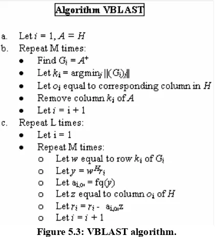
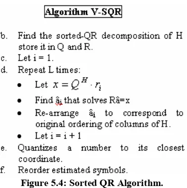
Figure 5.3: VBLAST algorithm. 53 Figure 5.4: Sorted QR Algorithm. 55 Figure 5.5: V-Least-Square algorithm. 56 Figure 5.6: BLER vs SNRavg M = 2; N = 4, 6 and 8 57
Figure 5.7: BLER vs SNRavg M = 8; N = 10 58
Figure 5.8: BLER vs SNRavg M = 8; N = 12 59
Figure 5.9: BLER vs SNRavg M = 8; N = 14 59
Figure 5.10: BLER vs SNRavg M = 2; N = 2 60
Figure 5.11: BLER vs SNRavg M = 4; N = 4 60
Figure 5.12: BLER vs SNRavg M = 6; N = 6 61
Figure 5.13: BLER vs SNRavg M = 8; N = 8 61
Figure 5.14: Computational Complexity vs SNRavg M = 2; N = 4 62
Figure 5.15: Computational Complexity vs SNRavg M = 2; N = 6 62
Figure 5.16: Computational Complexity vs SNRavg M = 2; N = 8 63
Figure 5.17: Computational Complexity vs SNRavg M = 8; N = 10 64
Figure 5.18: Computational Complexity vs SNRavg M = 8; N = 12 64
Figure 5.19: Computational Complexity vs SNRavg M = 8; N = 14 64
Figure 5.20: Computational Complexity vs SNRavg M = 2; N = 2 65
Figure 5.21: Computational Complexity vs SNRavg M = 4; N = 4 66
Figure 5.22: Computational Complexity vs SNRavg M = 6; N = 6 66
Figure 5.23: Computational Complexity vs SNRavg M = 8; N = 8 66
Figure 6.17: Computational Complexity vs SNRavg M = 8; N = 12 80 Figure 6.18: Computational Complexity vs SNRavg M = 8; N = 14 80 Figure 6.19: Computational Complexity vs SNRavg M = 2; N = 4 81 Figure 6.20: BLER vs SNRavg Comparison: CP Algorithm and new system for M = 2; N
= 4 83
Figure 6.21: Computational Complexity vs SNRavg: CP Algorithm and new system for M
= 2; N = 4 83
Figure 6.22: BLER vs SNRavg : CP Algorithm and new system for M = 8; N = 14 84 Figure 6.23: Computational Complexity vs SNRavg: CP Algorithm and new system for M
= 8; N = 14 84
Figure A.1: Channel capacity curve for receive diversity on a fast and block Rayleigh
fading channel with maximum ratio diversity combining. 91 Figure A.2: Achievable capacity for a MIMO slow Rayleigh fading channel versus SNR
for a variable number of transmit/receive antennas. 92 Figure A.3: Propagation model for a MIMO fading channel. 95 Figure A.4: Correlation coefficients in a fading MIMO channel with a uniformly
distributed direction of arrival a. 95 Figure A.5: The pdf of Rayleigh distribution normalized. 97 Figure A.6: The pdf of Rician normalized distributions with various K. 98 Figure A.7: BER performance comparison of coherent BPSK on AWGN and Rayleigh
fading channels. 99
FigureA.8: Delay transmit diversity scheme. 100 Figure A.9: BER performance of BPSK on Rayleigh fading channels with transmit
LIST OF TABLES
Table 6.17: Performance analyses for eight transmit and twelve receive antennas. 79 Table 6.18: Performance analyses for eight transmit and fourteen receive antennas. 79 Table 6.19: Performance analyses for two transmit and four receive antennas. 81 Table 6.20: Performance comparison: CP algorithm and new system for a 2x4 array. 82 Table 6.21: Computational Complexity comparison: CP algorithm and new system for a
2x4 array. 82
Table 6.22: Performance comparison: CP algorithm and new system for a 8x14 array. 83 Table 6.23: Computational Complexity comparison: CP algorithm and new system for a
8x14 array. 84
ACRONYMS
3G Third Generation of Communications 4G Fourth Generation of Communications AWGN Additive White Gaussian Noise
BER Bit Error Rate
BLAST Bell Labs Layered Space Time BLER Block Error Rate
BPSK Binary Phase Shift Keying CC Convolutional Channel Coding CDMA Code Division Multiple Access dB Decibels
DBLAST Diagonal Bell Labs Layered Space-Time DLST Diagonal Layered Space-Time
DSP Digital Signal Processor EGC Equal-Gain Combining
FPGA Field Programmable Gate Architecture GPRS General Packet Radio Service
GSM Global System for Mobile HLST Horizontal Layered Space-Time IC Integrated Circuits
IEEE Institute of Electrical and Electronics Engineers KZ Korkine-Zolotareff
LAN Local Area Network LLL Lenstra-Lenstra-Lovász LOS Line of Sight
LS Least Square
LST Layered Space-Time MEA Multiple Element Arrays
MIMO Multiple Input - Multiple Output ML Maximum Likelihood
MMSE Minimum Mean Square Error MRC Maximal Ratio Combining PDF Probability of Density Function PLD Programmable Logic Device QAM Quadrature Amplitude Modulation SI Spatial Interleaver
SINR Signal to Noise Interference Ratio
SINR0 Initial Signal to Noise plus Interference Ratio
SISO Single Input - Single Output SNR Signal to Noise Rate
STC Space Time Coding STBC Space-Time Block Codes STTC Space-Time Trellis Codes SVD Singular Value Decomposition TLST Threaded Layered Space-Time
VBLAST Vertical Bell Labs Layered Space Time VLST Vertical Layered Space-Time
1.
INTRODUCTION
Communications services have experienced and exponential increase in the past fifty years. Starting with the invention of transistor in 1947, and soon after the creation of integrated circuits (IC), the development of high integration technology, with small power requirements, low weight and high response speed were possible. This way, the creation of satellite communications in 1965 was made a reality [1], beginning with the era of wireless communication services.
At present time, wireless and mobile communication services are becoming a very important issue in information technology. We can highlight cellular and wireless networks (GSM – Global System for Mobile, CDMA – Code Division Multiple Access, IEEE802.11x and Hyperlan) as the main wireless and mobile communications means up to this day. These wireless technologies arose thanks to the simultaneous development of both digital communications techniques and semiconductor devices, which allow high integration circuit design of complex signal processing functions encountered in modern communications systems. Thus, efficient mobile communications systems are available, allowing the transmission of information which was unimaginable only ten years ago, and giving rise to huge economic implications (e-commerce, e-business, etc).
As a result, an explosion of new communication services came out, due to this important advance in wireless and mobile communications. Demands for capacity in wireless communications have been rapidly increasing worldwide in order to satisfy the requirements of these new services. Today, most fixed public communications services offer data, audio and multimedia communications. However, for mobile systems, things are not that easy since wireless channels present serious drawbacks of limited available spectrum, and capacity needs cannot be met without significant increase in the spectral efficiency (bit/sec/Hz) of these channels. The prime aspect in the further advance of wireless communications is inescapable: the development of new and efficient communications systems requires improved signaling schemes and a detailed and accurate measurement and characterization of the wireless channel [4].
in real time and with high quality [14]. As we can see, the trend of wireless systems is to converge in such a way that a communications system supporting both mobility and high data rates for multimedia services is to be available in the short term. This way, wireless systems will become an excellent alternative to the wired counterparts.
As an example, the new IEEE802.16 standard, also known as WiMAX (World Interoperability for Microwave Access) has been created to try to fulfill this requirement. It is claimed that it will support transmission speeds of up to 30 – 130Mb/s in the IEEE802.16 version, and up to 170Mb/s in the IEEE802.16a version. Moreover, it is expected that the coverage area will be of 2 kilometers in IEEE802.16 and up to 30 kilometers in IEEE802.16a, as opposed to the IEEE802.11b which can only offer coverage areas of 50 up to 150 m [15][16]. The considerable increase in bit rate in this new standard makes possible mobile systems with communications services similar to the wired counterpart, i.e. multimedia mobile communications. Nevertheless, it is evident that we need new technologies that make an efficient use of the spectrum, which derives in the need for transmission techniques offering high spectral efficiency. In this thesis, this need is addressed where new transmission techniques which are spectral efficient are investigated.
At the moment, different alternatives exist trying to achieve the design of communications systems with high spectral efficiency. Among these techniques, we can distinguish one that is potentially important and which uses arrangements of antennas at both, transmitter and receiver end. It is known as MIMO systems (Multiple Input – Multiple Output) [5][6].
The MIMO systems theory has demonstrated channel capacities that depend linearly on the number of antenna pairs utilized (in the transmitter and receiver side) [7]. Nevertheless, the detection procedure is very complex since this implies the knowledge of the channel’s spatial characteristics. Moreover, the omnidirectional multipath propagation and the Rayleigh fading models are no longer accurate in this kind of scenarios. This means that multiple antenna transmitters and receivers will not work properly if designed without a precise understanding of the spatial-temporal characteristics of the multipath channel.
The detection procedure in MIMO systems is generally known as Space-Time Coding (STC) [8]. MIMO systems were possible when space-time coding algorithms appeared. The principal idea of this approach is to jointly design modulation, coding and equalization. Space-Time coding can be divided into three types: Space-Time Block Codes (STBC) [8], Space-Time Trellis Codes (STTC)[9] and the so-called Bell Labs Layered Space-Time Architecture (BLAST) [10]. Layered Architectures are also referred to as Spatial Multiplexing techniques.
Among the different code techniques in space-time, the BLAST architecture is the one that has demonstrated the advantages of the MIMO systems in a practical way [17].
inappropriate for a hardware implementation. A simplified version of the DBLAST algorithm is the Vertical BLAST (VBLAST). This approach can reach tens of bits/s/Hz with multiple antennas and reduced complexity. In a VBLAST system, the uncoded data streams are demultiplexed into M substreams, each being transmitted simultaneously by one transmit antenna. At the receiver, the received signals from N received antennas are detected by a decision feedback algorithm. At present time, multiple realizations of the VBLAST exist whose aim is to reduce the computational complexity.
As stated above, the aim of this thesis is to analyze the so-called space-time coding systems for high-rate mobile communications systems. Specifically, one of the goals of this thesis is to analyze the VBLAST architecture from a performance-complexity standpoint. Different approaches of this algorithm are considered namely, the Singular Value Decomposition, the Sorted QR Decomposition and the LS algorithm [12]. These variants are compared to the near optimum Maximum Likelihood (ML) algorithm proposed by Agrell in [13]. This algorithm will be used as a reference to assess the performance of the different VBLAST approaches. This way, a selection of the VBLAST approach presenting the best tradeoff performance-complexity can be made and justified.
The second goal of this work is to envisage some improvements to the VBLAST algorithm without rendering it too complex. The main idea is to improve its performance, as compared to the conventional VBLAST and Agrell’s algorithms, while maintaining its complexity as reduced as possible, in order to consider a hardware implementation. This idea is carried out with the addition of a simple convolutional channel coder to the VBLAST architecture. At the receiver, this convolutional code is decoded by means of the Viterbi algorithm.
The document presents simulation results which compare Agrell’s algorithm and the VBLAST variants from a complexity and performance point of view. It will be shown that the LS algorithm achieves the best tradeoff. In addition, a new space-time coding scheme is proposed which comprises a convolutional code at the transmitter together with the BLAST encoder, and the Viterbi algorithm concatenated with the VBLAST decoder is used at the receiver. It is shown that this system can achieve a 2dB gain in terms of Block Error Rate (BLER) performance. The computational complexity was estimated and it is shown that a hardware implementation of this system is still possible.
six, the design of a simple space-time coding scheme consisting of a conventional channel coding scheme and the VBLAST algorithm is proposed so as to reduce the BLER performance of the overall system. Finally, conclusions and future work/perspectives are discussed in chapter seven.
REFERENCES
[1] J. G. Proakis, M. Salehi, “Communication Systems Engineering”, Second Edition, 2002.
[2] A. Paulraj, R. Nabar, D. Gore, “Introduction to Space-Time Wireless Communications”, Cambridge Editors, 2003.
[3] WI-FI Planet: The source for WI-FI business and technology. http://www.wi-fiplanet.com/tutorials/
[4] G. J. Foschini: “Layered space-time architecture for wireless communication in environment when using multiple antennas”. Bell Lab. Tech. J., 1996. I. (2), pp. 41-59. [5] M. Dobler, “Space-Time Trellis Codes for Hiperlan2”, IST-MIND Workshop. King’s College London, 7 Oct 2002.
[6] R. Gaspa, J. R. Fonollosa, “Comparison of Different Transmit Diversity Space-Time Code Algorithm”, Department of Singal Theory and Communications. Universitat Politecnica de Catalunya.
[7] A. Pascua, M. A. Lagunas, “Avances en Técnicas de Codificación Espacio-Temporal en Sistemas de Comunicaciones Móviles”, URSI 2002.
[8] S. M. Alamount, “A simple transmit diversity technique for wireless communications”, IEEE J. Sel. Arcas in Comm., pp. 1451 – 1458, Oct. 1998.
[9] V. Tarokh, H. Jafarkhani, A. R. Calderbank, “Space-time block codes for orthogonal designs”, IEEE Trans. On Inf. The., pp. 1456 – 1567, July 1999.
[10] G. J. Foschini, “Layered Space-time Architecture for wireless communications in a fading environment when using multiple antennas”, Bell Labs Technical Journal, Vol 1, No. 2, pp. 41 – 59, 1996.
[11] B. Vucetic, J. Yuan, “Space-Time Coding”, WILEY, 2002.
[12] M. Bazdresch, R. Guisantes: “Least-Squares Techniques Applied to VBLAST Receivers”. Admission in process.
[13] E. Agrell, T. Eriksson, A. Vardy: “Closest point search in Lattices”. IEEE Transactions on Information Theory. Vol. 48. No. 8. August 2002, pp. 2201 – 2214
[14] Z. Hunaiti, V. Garaj, W. Balachandran, F. Cecelja, “An Assessment of 3G link in a Navigation System for Visually Impaired Pedestrians”, 15th International Conference on Electronics, Communications and Computers, CONEILECOMP 2005, pp. 7-9.
[15] C. Kamath, “Hiperlan/2: High Performance Radio Local Area Network/2”, Presentation available on: http://www.llnl.gov/CASC/people/kamath/
[16] “802.11 Wireless Ethernet Standards”, http://stdsbbs.ieee.org/group/802.11
2
CHARACTERIZATION AND PERFORMACE OF
MULTIPLE-INPUT MULTIPLE-OUTPUT WIRELESS
COMMUNICATION SYSTEMS
2.1 INTRODUCTION
In this chapter concepts of multiple-input multiple-output (MIMO) versus single-input single-output communications systems (SISO) will be analyzed. In MIMO systems, signaling goes beyond simple antenna diversity. Data streams of symbols are broken and separated into M new sub-streams (where M is the number of transmit antennas) which determine the lower number of multipaths in the free space.
This chapter presents an introduction to MIMO concepts and signal processing, emphasizing the potential gains in channel capacity by increasing the spatial signals on the transmitter and receiver. The second part of the chapter presents a brief panorama of space-time coding techniques as a preview to the near-optimum closest point (CP) decoder algorithm which will be described in the next chapter. We will see that simpler suboptimum decoding techniques such as the BLAST algorithm are needed in order to render MIMO systems feasible. The major topics discussed in this section are listed below:
• Section 2.2: Characterization of MIMO channel
• Section 2.3: Channel capacity for conventional antenna arrays
• Section 2.4: Performance limits of MIMO systems
• Section 2.5: Introduction to Space-Time coding
• Section 2.6: Conclusions.
2.2 CHARACTERIZATION OF MIMO CHANNELS
MIMO systems are defined as an array of multiple antennas at both, receiver and transmitter. This kind of systems is also called MEA (Multiple Element Arrays) [4]. Systems with a single antenna at the transmitter and receiver can obtain excellent performance with conventional channel coding and optimized modulation techniques at the expense of increased bandwidth. Nevertheless, MIMO systems can obtain similar performance with a couple of antennas and simple modulation and without increasing bandwidth. This makes the system efficient and with low required transmit power.
are also synchronized, and use the same frequency band, which basically can be viewed as M virtual transmission channels with the same signal constellation. It is important to notice that in these systems the transmit power is divided into the M transmit antennas; therefore, the average symbol energy is the same. In a general MIMO system, any number of transmit and receive antennas can be used; however, in this thesis it is assumed that the number of received antennas is equal or greater than the number of transmit antennas, i.e. N ≥M. The channel is assumed to be frequency-flat with block Rayleigh fading (some Rician and fast Rayleigh fading characteristics are discussed in appendix A). This means that the channel impulse response is random but it remains constant during the transmission of a block. This block comprises L information symbols. In addition, the channel is corrupted by AWGN noise. These assumptions are not unrealistic since this scenario is usually encountered in indoor applications such as WLAN environments. Mathematically, the channel can be represented by the channel matrix H whose elements hij represent the link
between the i-th transmit antenna and the j-th receive antenna.
Next section will show us all the fundamentals of MIMO systems and some of the mathematical aspects. We must consider that for any WLAN system, the normal supposition is that distances are short and the fading is constant. Also, in indoor environments, line of sign is very rare, so it is correct and very close to reality consider block Rayleigh fading with AWGN noise.
2.2.1 BASIC DEFINITIONS AND FUNDAMENTALS
2.2.1.1 Multipath Propagation
In wireless communications, there are a lot of objects, such as houses, buildings, trees, which act as reflectors for the radio waves. They produce reflected waves with attenuated amplitudes and phases. As a modulated signal is transmitted, it could have reflections that create new waves with multiple directions and multiple propagation delays. These reflected waves are called multipath waves [7]. These multipath waves are collected by the receiver antenna at any point in space; they may be combined in a constructive or destructive form, depending on the random phases. The sum results in a spatially varying wave field. When the handset is moving, the receiver can get waves which vary widely in amplitude and phase, and when the handset is stationary, the amplitude variations are due to the movement of surrounding objects. This amplitude fluctuation of the received signal is called signal fading.
2.2.1.2 Doppler Shift
coming with an angle θ with respect to the direction of the vehicle motion. The Doppler shift denoted by fd is given by [15]
θ
cos *
c f v
f c
d = 2.1
where v is the speed of the vehicle and c is the speed of light. In a multipath propagation environment, the maximum Doppler shift is
c f v
f c
d
*
max = 2.2
This shift is referred to as maximum fade rate. As a result, the single tone transmitted gives rise to a received signal with a spectrum of nonzero width, which is called frequency dispersion of the channel.
2.2.1.3 Diversity
Diversity is used to reduce the multipath effects and improve the reliability of transmission without increasing the transmitted power or sacrificing bandwidth. This technique requires multiple replicas of the signal at the receiver.
The basic idea is that two or more independent samples of a signal are transmitted. These will fade in an uncorrelated manner, in such a way that some samples are severely faded while others are less attenuated. The probability of all the samples being simultaneously below a given level is lower than the probability of a single individual sample. Thus, combinations of the various samples result in a greatly reduced fading and improved reliability of transmission [9][10].
Diversity techniques are used in mobile communications in a number of ways in order to improve performance. According to the domain where diversity is introduced, the techniques are classified into time, frequency and space diversity. The reader is referred to appendix B for a more detailed discussion.
Now, we will discuss how these phenomenons are related to MIMO communications systems.
2.2.2 MIMO CHANNEL MATRIX.
∫
+∞∞ −
= H(τ(t)x(τ)dτ y(t) 2 1 2.3 where = ) ( ... ) ( ) ( 2 1 t y t y t y N y(t) , = ) ( ... ) ( ) ( 2 1 t x t x t x M x(t) , = ) , ( ... ) , ( ) , ( ... .... ... ) , ( ... ) , ( ) , ( ) , ( ... ) , ( ) , ( , , 2 , 1 2 , 2 , 2 2 , 1 1 , 1 , 2 1 , 1 t h t h t h t h t h t h t h t h t h N M N N M M τ τ τ τ τ τ τ τ τ t)
H(τ( 2.4
Matrix Hij(τ,t) is the channel impulse response of the virtual channel from the ith transmit
antenna to the jth receive antenna. For simplicity, as stated previously, if we assume block fading, the MIMO channel can be represented as a time invariant channel model. In this case, there is no frequency or time dependency in the channel; it results in a constant H matrix, which makes the estimation of the received signal as
) ( 2 1 )
(t Hx t
y = 2.5
2.2.3 PROCESSING THE MIMO SIGNAL.
The MIMO system is a complicated structure, whose better representation is based on matrix/vector analysis. Processing at the transmitter and receiver is needed in order to produce the set of received signals with highest overall capacity. All this operations will be discussed in a basic form in this section, and taking as a reference the block diagram shown in figure 2.1.
Figure 2.1: The matrix representation of signal processing operations in a MIMO system.
After the channel operates on the transmitted signal to produce HVx(t), the receiver operates in the incoming signal with matrix U’, so we get the final output signal vector
) ( 2
1
t x HV U' z(t)
D8
7 6
= 2.6
It is very important to remember that operator U’ is an NxN unitary matrix with the property U’U=I. This condition, as we saw, assures that we have not added or subtracted any signal power.
Now, let us propose an algorithm on the MIMO channel which makes that operation U’HV may be replaced by a diagonal matrix D. This new operation consists of diagonal elements, all of which are positive and constant. Matrices U and V are defined so that the transmission operation generates matrix D (recall that the number of transmit antennas must be lower or equal to the number of receive antennas N ≥M). This way, the estimation process at the receiver is greatly reduced.
Mathematically, this means that the MIMO channel can be viewed as a set of M separate channels from transmitter to receiver with the conditionN ≥M . If we have M > N the diagonal matrix would support a maximum of N separate channels. Thus, the number of separate channels with M transmit and N receive antennas ismin(M,N), which means that the number of separate channels is the minimum between M and N.
The signal processing steps described above can be done in several ways. In this thesis, we present four detailed descriptions: Maximum Likelihood (ML) based in the closest point algorithm and three variants of Vertical Bells Labs Layered Space-Time Architecture (VBLAST) [16]. They will be described in following chapters.
2.2.4 PHYSICAL INTERPRETATION OF MIMO CHANNELS
As we saw, a MIMO channel has the particular characteristic of creating separate virtual channels that depend only on the number of transmit and receive antenna pairs, which obviously is reflected in the channel capacity obtained by the system [19]
+
≈ * *log2 1 SINR0 M
N B
M
C 2.7
Notice that equation 2.7 is different to SISO systems because even though the SINR increases by a factor N/M, the overall capacity is multiplied by M channels. The main idea here is to transmit data using many different low-powered channels rather than using one single high-powered channel.
each bit in the frame will be transmitted by one transmit antenna. Each column in V contains the M amplitudes and phases for a symbol sent through the array of M transmit antennas. From matrix V is important to visualize that each antenna is defined by a unique spatial radiation pattern, so each of the columns have unique amplitudes and phase weightings. For instance, column 1 in V assigns a radiation pattern to x1(t), column 2
assigns a radiation pattern to x2(t), and so on.
Matrix U operates over the received signals from the N receiver antennas. Each column of U defines a radiation pattern that recognizes one of the original symbols sent by the transmitter (see Fig. 2.2). The weighting operation of V and U using unique antenna patterns to each separated data streams creates individual symbols from the others that come from the multipath channel allowing a correct estimation of each transmitted symbol by the corresponding receive antenna.
[image:33.612.105.512.332.690.2]Remember that multipath channel is very complicated in practice, and antenna patterns have finite resolution, so the MIMO processing can not be simplified with a few dominant scatters and get perfect separation of symbols; however the basic concept (which is the main propose of this sections) has been explained.
2.3 CHANNEL CAPACITY FOR CONVENTIONAL ANTENNA
ARRAYS
We have explained the fundamental concepts of MIMO systems and receive processing; however, the main question is the increase in the channel capacity achieved by these systems. This section discusses the performance of multiple antenna systems, starting from the SISO, SIMO and MISO systems, the ancestors of space-time block codes and MIMO architectures.
2.3.1 SINGLE-INPUT SINGLE-OUTPUT (SISO).
The simplest and the baseline for comparison will be SISO system, which is shown in figure 2.3. SISO systems use only one transmit antenna with PT input power. We can
estimate the Shannon channel capacity for this system by the expression [11]
(
0)
2 1
log SINR B
C = ⋅ + 2.8
[image:34.612.207.405.425.515.2]Where B is the available bandwidth and SINR0 is the average signal to noise plus interference ratio. Note that from digital communications theory, the available bandwidth limits the symbol rate, but not necessarily the bit rate. It is very common to forget that we can transmit more that one bit on a single complex baseband symbol. While symbols with more than two states are more susceptible to noise and interference, higher SINR makes reliable transmission possible and helps to approach Shannon capacity limit in systems.
Figure 2.3: A SISO antenna configuration.
2.3.2 SINGLE-INPUT MULTIPLE-OUTPUT (SIMO).
A SIMO system is shown in figure 2.4. N number of antennas are used at the receiver, producing N copies of the faded signal at the receiver. Although it is almost impossible, we must say that if N signals have the same amplitude, they can produce an N2 increase in signal power. Of course, there are not N sets of noise/interference that can add together as well. Noise and interference add incoherently (not with the same amplitude) to create an increase in noise power less that N. Therefore, the increase in SINR is [3]
[
]
[
]
02
NSINR ce
Interferen Noise
N
wer SignaltoPo N
SINR =
+
So, channel capacity for this system is approximately:
(
0)
2 1
log N SINR B
C≈ ⋅ + ⋅ 2.10
which is a little higher that SISO system. This difference at the receiver side implies an increase in the signal to noise interference ratio when multipath channels are used. As an example, when we are in open-space, the receiver antenna elements are phased together to form an array with maximum gain in the direction of signal arrival. This peak causes a subsequent increase in SINR and channel capacity. But if we are in a multipath channel, the direction of signal arrival may be dispersed throughout the azimuth. Figure 2.4 show the SIMO diagram.
Figure 2.4: A SIMO antenna configuration.
2.3.3 MULTIPLE-INPUT SINGLE-OUTPUT (MISO).
In this system (see Fig. 2.5), M antennas are used at the transmitter. The total transmitted power is split into M transmitters. This way, although the power per antenna drops, signals are transmitted in such a way that they add coherently at the receiver, producing a net M-fold increase in SINR, as compared to the SISO case. Since we have only one receiver, noise/interference power should be the same. The overall increase in SINR becomes [1]:
[
]
0 2
/
MSINR ce
Interferen Noise
M Power Signal
M
SINR ≡
+ −
≈ 2.11
The channel capacity for this system is [3]:
(
0)
2 1
log M SINR B
C ≈ ⋅ + ⋅ 2.12
Figure 2.5: A MISO antenna configuration.
2.3.4 MULTIPLE-INPUT MULTIPLE-OUTPUT (MIMO).
Finally, the general structure of a MIMO system is presented in figure 2.6. It consists of M transmit and N receive antennas. Signals are to be transmitted and received with such phasing as to maximize the total signal power through the wireless channel. The result is (approximately) an M*N-fold increase in the SINR of the received signal. The channel capacity for this kind of systems is given by
+
≈ * *log2 1 SINR0 M
N B
M
C 2.13
From this equation we can observe that maximum channel capacity is given when multiple-inputs and multiple-outputs are placed in the same system. A physical interpretation at open-space is that both transmitter and receiver use their multiple antennas in a phased array configuration, increasing the SINR substantially. When in a multipath scenario, in order to achieve the maximum channel capacity, transmit and receive diversity is used to achieve the highest possible SINR in the overall link.
Figure 2.6: A MIMO antenna configuration.
number of bits we can transmit is increased almost four times with respect to SISO systems. Also, the figure shows that when we introduce diversity at the receiver, the efficiency is increased faster that if the diversity is introduced at the transmitter. It must be noted that MIMO systems can be either square (same number of receive and transmit antennas) or not; but for this thesis, we assume that the number of transmit antennas is smaller or equal than the number of receive antennas.
Figure 2.7: Comparison between different kinds of array system.
2.4 FADING ASSUMPTIONS IN MIMO SYSTEMS
As we saw in last section, MIMO systems set individual channels between pairs of transmit and receive antennas, which are modeled by an independent flat Rayleigh fading process. In this section, we limit our attention to the analysis of the narrowband channels, so that they can be described by frequency flat models.
Rayleigh models are realistic for environments with a large number of scatterers. In channels with independent Rayleigh fading, a signal transmitted from every transmit antenna appears uncorrelated at each of the receive antennas. As a result, signals corresponding to every transmit antenna have a distinct spatial signature at the receive antenna [2].
estimated at the receiver but unknown at the transmitter. Furthermore, we assume that the elements of channel matrix are zero mean Gaussian complex random variables, each with variance of ½. So, each entry of the channel matrix has a Rayleigh distributed magnitude, uniform phase and expected magnitude square equal to unity, i.e.E
[ ]
hij 2 =1. The probability density function (PDF) for a Rayleigh channel with distributed random variable is z= z12 +z22 , where z1 and z2 are two statistically independent Gaussian randomvariables, each with zero mean and variance σr2 [3]
( )
2, 02
2
2 ≥
=
−
z e z z
p r
z
r
σ
σ 2.14
where σr2 is usually normalized to ½. According to how frequently the channel coefficients
change, three kinds of scenarios can be distinguished, namely
1. Fast Fading Channel. The entries in the channel matrix change randomly at the beginning of every symbol interval T and are constant during one symbol interval. 2. Block Fading Channel. The entries in the channel matrix are random and constant
during a fixed number of symbol intervals, which is shorter than the total transmission.
3. Slow or Quasi-Static Fading Channel. The matrix H is random but constant during transmission.
As indicated above, we will consider only block fading channels. Appendix A gives a more general treatment of fading channels in situations other than block fading.
2.5 INTRODUCTION TO SPACE-TIME CODING
In previous section we saw that information capacity of wireless communications systems can be increased considerably by employing multiple antennas at the transmitter and receiver, where capacity grows linearly with the minimum number of antennas.
One fact of wireless communications is inescapable: the development of new systems requires that the channel is measured and modeled to an increasingly higher degree of detail. We can no longer make approximations about the spatial channel, such as omni-directionality in the multipath propagation and Rayleigh fading. Multiple antenna transmitters and receivers will not function properly if designed without an understanding of the spatio-temporal characteristics of the multipath channel.
Advances in channel coding make it possible to approach Shannon capacity limits [17] in systems with single antenna links (Single Input – Single Output) [19]. However, as we described in previous paragraphs, even more significant improvements can be achieved with MIMO channels. It has been demonstrated that cellular SISO systems can achieve spectral efficiencies between 1-2 bits/sec/Hz whereas MIMO systems with 8 antennas at each side can obtain 37 bits/sec/Hz at an SNR of 20 dB [20].
In order to approach those capacities, MIMO channels employ space-time coding [5][6]. Space-time coding techniques are used with multiple antenna arrays. Coding is performed in spatial and temporal domains, spatial domain means multiple antennas and temporal domain means various time slots or time periods. The spatial correlation is used to exploit the MIMO channel fading and minimize transmission errors at the receiver. This kind of transmission can achieve transmit diversity and power gain over uncoded systems without sacrificing the bandwidth. There are basically three types of coding structures: space-time block codes (STBC)[18], space-time trellis code (STTC) [13] and space-time layered codes (LST) [16]. A general space-time coding system is shown in figure 2.8. The main process in all schemes is the exploitation of the multipath and to obtain performance gains [8].
SPACE-TIME ENCODER
SPACE-TIME DECODER
x1
x2
xM
r1
r2
rN
h11
h12
h21
hN1
h22
hN2
h1M
h2M
hNM
2.8: General scheme of a space-time system
2.5.1 SPACE-TIME BLOCK CODES (STBC)
The first space-time coded system was created by Alamount [18] (figure 2.9). The general idea is to consider as input to the encoder a group of k symbols transmitted at different time slots. This can be seen as arranging the symbols into a code matrix, where columns represent the symbols transmitted by one of the transmit antennas and rows represent the time intervals of transmission (see figure 2.9). The code rate of the system is defined as
p k
r = / ; where p is the number of transmission intervals and k is the number of transmit antennas (number of columns in the code matrix).
Figure 2.9: Coding and Decoding Alamount System.
2.5.2 SPACE-TIME TRELLIS CODES (STTC)
The second type of space-time coding systems were proposed by Tarok et al. [11] and called STTC (see figure 2.10). STTC develop channel coding, modulation and transmit diversity simultaneously. The system can obtain important gains but with increased bandwidth; in addition, compared to STBC, its complexity is much higher [8].
Figure 2.10: Coding and Decoding Tarok system.
2.5.3 LAYERED SPACE-TIME CODES (LST)
LST codes were proposed by Foschini in the 80’s [16]. In order to increase the bit rate in the systems, LST introduced an array of MxN antennas, each one of them transmits a sub-stream. Consider the example of a 3x3 antenna array.
The 3x3 MIMO system is shown in Figure 2.11. In order to increase the bit rate, the input stream is introduced to the demultiplexer, which creates at its output three new data sub-streams, each with equal number of bits. The data sub-streams are arbitrarily coded onto digital symbol streams. For sake of simplicity, the constellation used is BPSK (Binary Phase Sift Keying).
It is possible to take these three data streams and modulate them directly to the carrier frequency and send them out through the transmit antennas, but the basic problem here is the presence of low-powered channels through one or more of the transmit antennas. The channels can not be separated with equal SINR at the receiver by simple inversion of the channel matrix H. We need a channel estimation feedback because the transmitter has no way to know which of the separate channels is able to support the data rate of the transmitted streams.
In order to solve this problem, Foschini introduced a transmitter architecture that cycles the sub-streams [16]. Each transmitted stream takes turn through one of the transmit antennas, spending a time-slot at each antenna element and cycling back to its original antenna element every three time slots. After sufficiently large time slots, each transmitted data stream experiences the same average channel conditions, which can be viewed as being transmitted with equal power.
When information has passed through the channel, each stream is detected from the receive antennas, one at a time. For antenna one, the algorithm extracts the first signal according to the expression [1]
[
]
( )[
1 0 0]
( )) ( )
( 1
1 t u y t u H H H x t x t
x = ⋅ = 1 ⋅ 1 2 3 = 2.14
We apply this equation to the other two receive antennas. However, we can obtain signal gain through interference cancellation. Since we already knowx1, this value is subtracted from vectory(t). Next expression shows how the process is affected with this
[
0]
( )[
0 1 0]
( )) ( )
( 2
2 t u y t u H H x t x t
x = ⋅ = 1 ⋅ 2 3 = 2.15
We can note that the decision criterion is diminished in one less interferer. A simple point of view is that we are solving a linear equation system; thus, removal of the first estimated symbol provides an extra degree of freedom for constructingu1. Since two independent estimates are available, the system can use combining algorithms to achieve diversity gain. The potential performance for this second data stream is equivalent to maximum ratio combining (MRC) diversity using two branches [12].
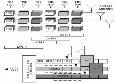
Figure 2.12 shows the signal extraction with interference cancellation at the receiver. As we can observe, the receiver buffers the incoming streams and extracts them in steps, each of them with duration of one time slot. At every step, the receiver detects a layer of data and spans other three time slots when the receiver has returned to detect the layer corresponding to stream 1.
The layers are decoded and multiplexed onto a final stream of output data. When the receiver detects stream 1, each time slot has had a different interference removed from the data stream. In time slot 1, two other layers have been subtracted during previous time slots, so this layer contains the most reliable data for layer 1. In time slot 3, none of the other layers have been subtracted, so this layer is the least reliable layer.
Figure 2.12: 3x3 MIMO system with Layered Architecture
2.6 CONCLUSIONS
In this chapter, MIMO systems have been defined as arrays of antennas in both transmitter and receiver, which can let us achieve performance improvements in both bit error rate and bit rates that other systems cannot obtain. The most important characteristic of these systems is diversity in space and time. Those techniques, applied together, let systems transmit information by multiple antennas and multiple slots of time. The diversity and multipath fading channel performance have been analyzed.
REFERENCES
[1] G. D. Durgin, ”Space-Time Wireless Channels”, Prentice Hall PTR. 2003.
[2] P. VanRooyen, “Advances in Space-Time Processing techniques open up mobile APPS”, EE Times, Nov. 8, 2002. http://www.commsdesign.com/story/OEF20021107S0021
[3] B. Vucetic, J. Yuan, “Space-Time Coding”. WILEY. 2004.
[4] D. Chizhik, G. J. Foschini, M. J. Gans, R. A. Valenzuela, “Keyholes, Correlations and Capacities of Multiantenna Transmission and Receive Antennas “, IEEE Transactions on Wireless Communications, Vol. 1, No. 2, April 2002.
[5] V. Tarokh, N. Seshadri and A.R. Calderbank, “Space-time codes for high data rate wireless communications: performance criterion and code construction”. IEEE Trans. Inform. Theory, vol. 44, no. 2, pp. 744-765. Mar. 1998.
[6] N. Seshadri, V. Tarokh, A. R. Calderbank, “Space-Time Codes for Wireless Communications: Code Construction”, 0-7803-3659-3, 1997.
[7] J. G. Proakis, “Digital Communications”, 4th Ed., Mc. Graw-Hill, New York, 2001. [8] V. Tarokh, A. Naguib, N. Seshadri, A. R. Calderbank, “Space-Time Codes for High Data Rate Wireless Communication: Performance Criteria in the Present of Channel Estimation Errors, Mobility and Multiple Paths”, IEEE Transactions on Communications, Vol. 47, No. 2, February 1999.
[9] K. F. Lee and D. B. Williams, “A Space-Frequency Transmitter Diversity Technique for OFDM Systems,” in Proc. IEEE GLOBECOM, EU, November 2000, pp. 1473-1477.
[10] Michigan Technological University, 2001.
http://www.geocities.com/hansadhwani8/smartantennas/diversity.html
[11] V. Tarokh, H. Jafarkhani, R. Calderbank, “Space-Time Block Coding for Wireless Communications: Performance Results”, IEEE Journal on Selected Areas in Communications, Vol. 17, No. 3, March 1999.
[12] M. A. Fkirin, A. F. Al-Madhari, “Prediction of time-varying dynamic processes”, The international Journal of Quality & Reliability, Vol. 14, iss. 5, pp. 505, 1997.
[13] Z. Hong, K. Liu, A. M. Sayeed, R. W. Hearth Jr., “A General Approach to Space-Time Trellis Codes”, Office of Naval Research #N00011-01-1-0825 and National Science Foundation CCR-9875805.
[14] www.mathcad.com
[15] H. D. Young, R. A. Freeman, “University Physics”, Addison-Wesley Publishing Company. INC. 1996.
[16] G. J. Foschini, “Layered Space-time Architecture for wireless communications in a fading environment when using multiple antennas”, Bell Labs Technical Journal, Vol 1, No. 2, pp. 41 – 59, 1996.
[17] C. E. Shannon, “Mathematical Theory of Communications”, University of Illinois Press, 1963.
[18] S. M. Alamount, “A simple transmit diversity technique for wireless communications”, IEEE J. Sel. Arcas in Comm., pp. 1451 – 1458, Oct. 1998.
[19] L. Hanzo, T. H. Liew, B. L. Yeap, “Turbo Coding, Turbo Equialisation and Space-Time Coding for Transmission Over Fading Channels”, John Wiley & Sons. 2002.
3
MAXIMUM LIKELIHOOD DETECTION OF SPACE-TIME
CODING SYSTEMS
3.1 INTRODUCTION
In this chapter, we consider the mathematical framework for Maximum Likelihood (ML) decoding of space-time coded systems. Matrix computation concepts will be highlighted and used to search for the correct signal sent from the transmitter to the receiver in a ML criterion. ML decoding is the optimum procedure for computing the point
−
x in a lattice which is closest to the received symbol, x. Nevertheless, this procedure is extremely complex, giving rise to suboptimum algorithms among which we can find the BLAST algorithm for Layered Space-Time coding. Hence, the aim of this chapter is to introduce the Closest Point (CP) decoding algorithm proposed by Agrell [2] and analyze its performance and complexity in order to elucidate the reasons why BLAST algorithm is the preferred choice for decoding Layered Space-Time coded systems. It is important to notice that CP uses all the lattice points in the space and ML decoding uses only the lattice points that belong to the constellation points in use. ML decoding is extremely complex to implement when the number lattice points is high; that is the reason why CP algorithms are commonly used since they can be seen as a suboptimum but a very good approximation to ML decoding with much less computational effort.
The outline of the chapter is the following
• Section 3.2: Introduction to Lattice points.
• Section 3.3: Preliminary of lattice calculations.
• Section 3.4: Agrell algorithm
• Section 3.5: Performance of CP algorithm.
• Section 3.6: Conclusions.
3.2 INTRODUCTION TO LATTICE POINTS
As an introduction, we can say that a lattice code is a finite subset of points of a lattice set (or of a lattice translate) within a bounded region containing the origin, so that the energy of each signal is bounded [1]. The lattice points are used to create the constellations points in the modulation process and attain the Shannon capacity bound.