Tag Clustering a New Cooperative Algorithm for Topology Organization in Ad-Hoc Networks-Edición Única

Instituto Tecnológico y de Estudios Superiores de Monterrey Campus Monterrey

Lic. Arturo Azuara Flores:

Director de Asesoría Legal del Sistema

", en los sucesivo LA OBRA, en virtud de lo cual autorizo a el Instituto Tecnológico y de Estudios Superiores de Monterrey (EL INSTITUTO) para que efectúe la divulgación, publicación, comunicación pública, distribución y reproducción, así como la digitalización de la misma, con fines académicos o propios al objeto de EL INSTITUTO.

El Instituto se compromete a respetar en todo momento mi autoría y a otorgarme el crédito correspondiente en todas las actividades mencionadas anteriormente de la obra.

De la misma manera, desligo de toda responsabilidad a EL INSTITUTO por cualquier violación a los derechos de autor y propiedad intelectual que cometa el suscrito frente a terceros.

Monterrey, Nuevo León a de 200

Tag Clustering a New Cooperative Algorithm for Topology

Organization in Ad-Hoc Networks-Edición Única

Title Tag Clustering a New Cooperative Algorithm for Topology Organization in Ad-Hoc Networks-Edición Única

Authors José Antonio Cervantes y Ramírez

Affiliation ITESM-Campus Monterrey

Issue Date 2005-12-01

Item type Tesis

Rights Open Access

Downloaded 19-Jan-2017 12:37:21

INSTITUTO TECNOLÓGICO Y DE ESTUDIOS

SUPERIORES DE MONTERREY

CAMPUS MONTERREY

Escuela de Tecnologías do Información y Electrónica Programa de Graduados

Thesis

Tag Clustering A New Cooperative Algorithm For Topology Organization in Ad-Hoc Networks

by

Ing. José Antonio Cervantes y Ramírez

Tag Clustering A New Cooperative Algorithm For

Topology Organization in Ad-Hoc Networks

by

Ing. José Antonio Cervantes y Ramírez

Thesis

Presented to the graduate program of the

Escuela de Tecnologías de Información y Electrónica

as a partial fulfillment of the requeriments for the degree of

Master of Science

major in

Telecommunications

Instituto Tecnológico y de Estudios Superiores de Monterrey

Campus Monterrey

Instituto Tecnológico y de Estudios Superiores de

Monterrey

Campus Monterrey

Escuela de Tecnologías de Información y Electrónica

Programa de Graduados

The members of the thesis committee recommended the acceptance of the thesis of José Antonio Cervantes y Ramírez as a partial fulfillment of the requeriments for the

degree of: Master of Science, major in:

Telecommunications

Thesis committee:

Ph.D. César Vargas Rosales Thesis advisor

Ph.D. José RamÓTi Rodríguez Cruz Ph.D. Jorge Carlos Mex Perera

Synodal Synodal

This work is dedicated with love:

Acknowledgements

To my parents Benjamín Cervantes y Castro and Maria Antonieta Ramírez de Cervantes, for their unconditional support throughout my life. To my brother Juan Manuel Cervantes y Ramirez for his support at any moment.

I am very grateful to my thesis advisor Cesar Vargas Rosales, Ph.D., for all his time during which we worked together, for all his professional advice for the accom-plishment of this work and for his friendship. Because, without his guidance this thesis would not have been possible. Also I want to thank to Jose Ramon Rodriguez Cruz, Ph.D., and Jorge Carlos Mex Perera, Ph.D., for their valuable comments for the en-hancement of this work.

To the ITESM and CONACYT for giving me the opportunity of realize my grad-uate studies.

I want to thank all my friends at GET, specially Pepe, Jeremías, Fernando, Paco, Victor, Fabian and Brenda. To my friends from Oaxaca Yalina, Eduardo, Gerardo, Gustavo, Ivan, Jose Luis and Himer for their friendship and helping at any moment.

JOSE ANTONIO CERVANTES Y RAMíREZ

Contents

Acknowledgements v

Abstract vi

Abstract vii

List of Tables x

List of Figures xi

Chapter 1 Introduction 1 1.1 Objective . 2 1.2 Justification 2 1.3 Contribution 2 1.4 Organization 3

Chapter 2 Wireless Ad-Hoc Networks 4 2.1 Typical Operational Characteristics 4 2.2 Routing in Ad Hoc networks 6 2.3 Types of Ad Hoc Mobile Communications 7 2.4 Shortest Path Algorithms 8 2.4.1 Dijkstra Algorithm 8 2.5 Clustering, [1] 9 2.6 Multi-cluster network architecture and clustering Algorithm 11 2.6.1 Lowest-ID Cluster Algorithm 12 2.6.2 Lowest-ID heuristic 12 2.6.3 Highest-Connectivity Cluster Algorithm 13 2.6.4 Highest-Degree heuristic 14 2.6.5 Properties Of The Two Cluster Algorithms 15

Chapter 3 Model Description 16 3.1 Analogy with the Basketball Game 16 3.2 Statistics in the Tag Clustering 21

3.3 Tag clustering Algorithm 23

Chapter 4 Performance Evaluation 28

4.1 Proposed Scenarios 29 4.1.1 Scenario 1 30 4.1.2 Scenario 2 33 4.2 Finding the Shortest Path 38 4.3 Communication Overhead 39 4.4 Tag Clustering Algorithm vs Different Clustering Algorithms 42

Chapter 5 Conclusion and Further Research 43

5.1 Conclusions 43 5.2 Further Research 44

Bibliography 46

List of Tables

4.1 Static Results for 3600 seconds 29 4.2 Static Results for different node density 31 4.3 Static Results for different communication range 34 4.4 Movement Results for different node density (speed 3 to 10 m/s) . . . . 35 4.5 Movement Results for different node density and speed 39 4.6 Summary of Different Clustering Algorithms 42

List of Figures

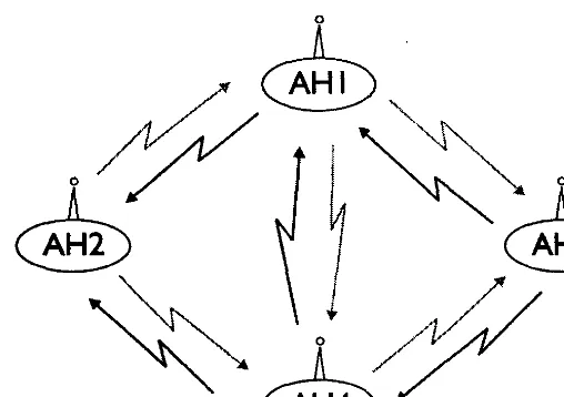
2.1 Ad hoc Wireless Network 5 2.2 At an airport, where people can access local- and wide-area networks,

ad hoc Blutooth connections are used to interconnect carried devices, such as PDAs, WCDMA mobile phones and notebook computers. For instance, a user might retreive e-mail via a HiperLAN/2 interface to a notebook computer, but read messages and reply to them via his or her PDA 7 2.3 Basic idea of Dijkstra's algorithm. At the kth step we have the set P of

the k closest nodes to node 1 as well as the shortest distance Di from node 1 to each node i in P. Of all paths connecting node 1 to some node not in P, the shortest one must pass exclusively through nodes in

P (since dij > 0) 9

2.4 The Link-Clusterhead Architecture 10 2.5 Example of clustering 11 2.6 Example of cluster formation (lowest-ID) 12 2.7 Example of cluster formation (highest-connectivity) 14

3.1 Basketball Game 17 3.2 Clustering Ad-hoc network 17 3.3 Best basketball players and their statistics 19 3.4 Ideal Tag Clusterig 22 3.5 Formation of clusters in tag clustering algorithm 26 3.6 Tagging nodes in tag clustering algorithm 27

4.9 Shortest Path communication range 200m without clustering 40 4.10 Shortest Path communication range 150m without clustering 41 4.11 Shortest Path communication range 150m with tag clustering 41

Tag Clustering A New Cooperative Algorithm For

Topology Organization in Ad-Hoc Networks

José Antonio Cervantes y Ramírez, M.Sc.

Instituto Tecnológico y de Estudios Superiores de Monterrey, 2005

Thesis advisor: Ph.D. César Vargas Rosales

Tag Clustering A New Cooperative Algorithm For

Topology Organization in Ad-Hoc Networks

José Antonio Cervantes y Ramírez, M.Sc.

Instituto Tecnológico y de Estudios Superiores de Monterrey, 2005

Thesis advisor: Ph.D. Cesar Vargas Rosales

Chapter 1

Introduction

Ad hoc wireless networks consist of mobile nodes interconnected by multihop com-munication paths. Unlike conventional wireless networks, ad hoc networks have no fixed network infrastructure or administrative support. The topology of the network changes dynamically as mobile nodes join or depart the network or radio links between nodes become unusable. Ad hoc wireless networks are creating, organizing, and self-administering. They come into being solely by interactions among their constituent wireless mobile nodes, and only such interactions are used to provide the necessary control and administration functions supporting such networks.

The ad hoc wireless networks offer unique benefits and versatility for certain envi-ronments and certain applications. No preexisting fixed infrastructure, including base stations, being prerequisite, they can be created and used "any time, anywhere." Sec-ond, such networks could be intrinsically fault-resilient, for they do not operate under the limitations of a fixed topology. Indeed, since all nodes are allowed to be mobile, the composition of such networks is necessarily time-varying. Addition and deletion of nodes occur only by interactions with other nodes; no other agency is involved. Such perceived advantages elicited immediate interest in the early days among military, po-lice, and rescue agencies in the use of such networks, especially under disorganized or hostile environments, including isolated scenes of natural disaster and armed con-flict. In recent days, home or small office networking and collaborative computing with laptop computers in a small area (e.g., a conference or classroom, single building, con-vention center) have emerged as other major areas of potential application. In addition, people also recognize that ad hoc networking has obvious potential application in all the traditional areas of interest for mobile computing.

The absence of fixed infrastructure means that the nodes of an ad hoc network com-municate directly with one another in a peer-to-peer fashion. The mobility of these nodes imposes limitations on their power capacity, and hence on their transmission range; indeed, these nodes often must satisfy stringent weight limitations for portabil-ity. Assuming ubiquitous IP networking as the underlying model for our discussion, it is evident that each node must therefore be able to function as a router as well. As the nodes move in and out of range with respect to other nodes, including those oper-ating as routers, the instantaneous topology changes must somehow be communicated to all other nodes as appropriate. In accommodating the communication needs of the user applications, the limited bandwidth of wireless channels and their generally hostile transmission characteristics impose additional constraints on how much administrative and control information may be exchanged, and how often. Ensuring effective routing is one of the great challenges for ad hoc networking, [13].

1.1 Objective

The objective of this thesis is to develop a cooperative topology organization algo^ rithm based on clustering concepts to allow network topology control and to evaluate the performance of ad hoc networks with respect to the organization, connectivity and mobility of the nodes, using the statistics proposed in the tag clustering algorithm.

1.2 Justification

The ad hoc networks are systems of fast implementation that do not count on permanent physical infrastructure. Therefore, it is recovery to obtain the interconnec-tions of nodes source and destination, and necessary to establish topologies on which the routes are constructed that will transport the information. However, given the ample class of stations (fixed, semi-portable, mobiles), it is necessary to study the way in which the nodes will be organized to be able to define a topology, and the necessary connectivity for its operation, formation and maintenance.

1.3 Contribution

We propose a new algorithm for ad-hoc networks, with the introduced concepts of collaborative work with the purpose of improving organization, connectivity and mobility of ad-hoc networks.

1.4 Organization

Chapter 2

Wireless Ad-Hoc Networks

A mobile ad hoc network is a network formed without any central administration which consists of mobile nodes that use a wireless interface to send packet data. Since the nodes in a network of this kind can serve as routers and hosts, they can forward packets on behalf of other nodes and run user applications. As we can see in Figure 2.1

In contrast to traditional wire-line or wireless networks, an ad hoc network could be expected to operate in a network environment in which some or all the nodes are mobile.

In this dynamic environment, the network functions must run in a distributed fashion, since nodes might suddenly disappear from, or show up in, the network. In general, however, the same basic user requirements for connectivity and traffic delivery that apply to traditional networks will apply to ad hoc networks, [9].

/

2.1 Typical Operational Characteristics

Distributed operation: a node in an ad hoc network cannot rely on a network

in the background to support security and routing functions. Instead these functions must be designed so that they can operate efficiently under distributed conditions.

Dynamic network topology: in general, the nodes will be mobile, which sooner

or later will result in a varying network topology. Nonetheless, connectivity in the net-work should be maintained to allow applications and services to operate undisrupted. In particular, this will influence the design of routing protocols. Moreover, a user in the ad hoc network will also require access to a fixed network (such as the Internet) even if nodes are moving around. This calls for mobility management functions that allow network access for devices located several radio hops away from a network access point.

Fluctuating link capacity: the effects of high bit-error rates might be more

Figure 2.1: Ad hoc Wireless Network

found in a multihop ad hoc network, since the aggregate of all link errors is what affects a multihop path. In addition, more than one end-to-end path can use a given link, which if the link were to break, could disrupt several sessions during periods-of high bit-error transmission rates. Here, too, the routing function is affected, but ef-ficient functions for link layer protection (such as forward error correction, FEC, and automatic repeat request, ARQ) can substantially improve the link quality.

Low-power devices: in many cases, the network nodes will be battery-driven, which

will make the power budget tight for all the power-consuming components in a device. This will affect, for instance, CPU processing, memory size/usage, signal processing, and transceiver output/input power. The communication-related functions (basically the entire protocol stack below the applications) directly burden the application and services running in the device. Thus, the algorithms and mechanisms that implement the networking functions should be optimized for lean power consumption, so as to save capacity for the applications while still providing good communication performance.

Besides achieving reasonable network connectivity by using multihop routes, the in-troduction of multiple radio hops might also improve overall performance, given a constrained power budget. Today, however, this can only be realized at the price of more complex routing, [9].

r

operation.

To further improve user perception of the service, user applications that run over an ad hoc network could be made to adapt to sudden changes in transmission quality. QoS support in an ad hoc network will affect most of the networking functions, especially routing and mobility. In addition, local buffer management and priority mechanisms must be deployed in the devices in order to handle differentiated traffic streams, [9].

2.2 Routing in Ad Hoc networks

For mobile ad hoc networks, the issue of routing packets between any pair of nodes becomes a challenging task because the nodes can move randomly within the network. A path that was considered optimal at a given point in time might not work at all a few moments later. Moreover, the stochastic properties of the wireless channels add to the uncertainty of path quality. The operating environment as such might also cause problems for indoor scenarios-the closing of a door might cause a path to be disrupted.

Several routing protocols have been proposed for these networks recently. These rout-ing protocols can be classified into three main categories: proactive, reactive and hybrid.

Traditional routing protocols are proactive in that they maintain routes to all nodes, including nodes to which no packets are being sent. They react to any change in the topology even if no traffic is affected by the change, and they require periodic control messages to maintain routes to every node in the network. The rate at which these control messages are sent must reflect the dynamics of the network in order to main-tain valid routes. Thus, scarce resources such as power and link bandwidth will be used more frequently for control traffic as node mobility increases, [9].

An alternative approach involves establishing reactive routes, which dictates that routes between nodes are determined solely when they are explicitly needed to route packets. This prevents the nodes from updating every possible route in the network, and instead allows them to focus either on routes that are being used, or on routes that are in the process of being set up.

The hybrid protocols use features of both reactive and proactive protocols. Non-clustered routing protocols have a flat routing architecture where each mobile node maintains complete routing information. Therefore they have routing overhead, which increases considerably with the network size. The main advantage of hybrid protocols is their flexibility in allowing the use of different routing mechanisms within and

Access Point

PDA

Cell phone

Laptop

Figure 2.2: At an airport, where people can access local- and wide-area networks, ad hoc Blutooth connections are used to interconnect carried devices, such as PDAs, WCDMA mobile phones and notebook computers. For instance, a user might retreive e-mail via a HiperLAN/2 interface to a notebook computer, but read messages and reply to them via his or her PDA.

tween clusters. Several routing protocols based on clustering architecture have been proposed in recent years. Organizing clusters hierarchically reduces routing overhead and increases scalability, [6].

2.3 Types of Ad Hoc Mobile Communications

Ad-hoc networking covers multihop scenarios, where network nodes communicate via other network nodes, such as conference, hospital, battlefield, rescue, and moni-toring scenarios. Particular ad hoc networks systems include packet radio networks, sensor networks, personal communication systems, rooftop (mesh) networks for wire-less internet access, and wirewire-less local area networks. Ad hoc networks may consist of self-organized standalone nodes, or can be linked to a fixed infrastructure via access point (such networks are also called hybrid ad hoc networks),[5].

doc-uments or presentations; business cards would automatically find their way into the address register on a laptop and the number register on a mobile phone; as commuters exit a train, their laptops could remain online; likewise, incoming email could now be diverted to their PDAs; finally, as they enter the office, all communication could auto-matically be routed through the wireless corporate campus network.

Today, our vision of ad hoc networking includes scenarios such as those depicted in Figure 2.2, where people carry devices that can network on an ad hoc basis. A users devices can both interconnect with one another and connect to local information points for example, to retrieve updates on flight departures, gate changes, and so on. The ad hoc devices can also relay traffic between devices that are out of range. The airport scenario thus contains a mixture of single and multiple radio hops.

These examples of spontaneous, ad hoc wireless communication between devices might be loosely defined as a scheme, often referred to as ad hoc networking, which allows devices to establish communication, anytime and anywhere without the aid of a central infrastructure. Actually, ad hoc networking as such is not new, but the setting, usage and players are. In the past, the notion of ad hoc networks was often associated with communication on combat fields and at the site of a disaster area; the scenario of ad hoc networking is likely to change, as is its importance, [9].

2.4 Shortest Path Algorithms

Due to the nature of routing applications, we need flexible and efficient shortest path procedures, both from a processing time point of view and also in terms of the memory requirements. Shortest Path problems are among the most studied network flow optimization problems, with interesting applications in a range of fields. One such application is in the field of ad hoc networks routing systems. Conventional techniques for solving shortest paths routing algorithms have been based on Dijkstras Shortest Path algorithm.

2.4.1 Dijkstra Algorithm

This algorithm requires that all arc lengths be positive (fortunately, the case for data networks applications). The general idea is to find the shortest paths in order to increasing path length. The shortest of the shortest paths from node 1 must be the single-arc path to the closest neighbor of node 1, since any multiple-arc path must be longer than the first arc length because of the positive length assumption. The next shortest paths must either be the single-arc path to the next closest neighbor of 1 or the shortest two-arc path through the previously chosen node, etc. To formalize this

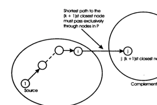
Shortest path to the (k + 1 )st closest node must pass exclusive)/ through nodes in P

Set P of K closest nodes to node 1

Figure 2.3: Basic idea of Dijkstra's algorithm. At the kth step we have the set P of the k closest nodes to node 1 as well as the shortest distance Di from node 1 to each node i in P. Of all paths connecting node 1 to some node not in P, the shortest one must pass exclusively through nodes in P (since dtj > 0).

procedure into an algorithm, we view each node i as being labeled with an estimate Di of the shortest path length from node 1. When the estimate becomes certain, we regard the node as being permanently labeled, and keep track of this with, with a set P of permanently labeled nodes. The node added to P at each step will be the closest to node 1 out of those that are not yet in P. Figure 2.3 illustrates the main idea. The detailed algorithm is as follows, [4]:

Initially P = {!}, DI = 0, and Dj = dy for j ^ 1.

Step 1. (Find the next closest node.) Find i e P such that

A = minjepDj (2.1)

Set P := P U {i}. If P contains all node then stop; the algorithm is complete.

Step 2. (Updating of labels.) For all; 6 P set

Go to Step 1.

(2.2)

2.5 Clustering, [1].

Oidinaty Node

dustertiead

Figure 2.4: The Link-Clusterhead Architecture

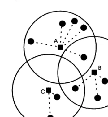
nodes that cover all mobile nodes in the network. Clusters can be either distinct or overlapping. In the former, each node belongs to only one cluster while in the latter, the neighboring clusters can have a common node (gateway) between them, [6].

Each cluster contains a clusterhead, one or more gateways, and zero or more ordi-nary nodes that are neither clusterheads nor gateways as shown in Figure 2.4. The clusterhead schedules transmissions and allocates resources within the clusters. Gate-ways connect adjacent clusters. A gateway may directly connect two clusters by acting as a member of both, or it may indirectly connect two clusters by acting as a member of one and forming a link to a member of the other, [12].

Most hierarchical clustering architectures for mobile radio networks are based on the concept of clusterhead The clusterhead acts as a local coordinator of transmissions within the cluster. It differs from the base station concept in current cellular systems, in that it does not have special hardware and in fact is dynamically selected among the set of stations. However, it does extra work with respect to ordinary stations, and therefore it may become the bottleneck of the cluster.

Clustering offers several advantages in mobile ad hoc networks. First, network par-titioning improves routing and mobility management,[14]. It increases system capacity, reduces signaling and control overhead and minimizes network congestion. This makes the network more scalable and enables support for larger network sizes. Second, cluster-ing stabilizes the network topology and provides a virtual infrastructure for a dynamic network. Here, the clusterhead acts as a base station for its cluster. Third, clustering helps to perform more efficient resource allocation. By assigning different codes to each

Figure 2.5: Example of clustering

cluster, MAC resource management can be improved and the wireless channel can be used efficiently,[7],[3].

2.6 Multi-cluster network architecture and

cluster-ing Algorithm

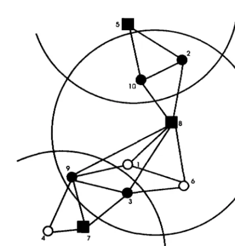
Figure 2.6: Example of cluster formation (lowest-ID)

2.6.1 Lowest-ID Cluster Algorithm

Each node is assigned a distinct ID. Periodically, the node broadcasts the list of nodes that it can hear (including itself).

• A node which only hears nodes with ID higher than itself is a "clusterhead" (CH).

• The lowest-ID node that a node hears is its clusterhead, unless the lowest-ID specifically gives up its role as a clusterhead (deferring to a yet lower ID node).

• A node which can hear two or more clusterheads is a "gateway". • Otherwise, a node is an ordinary node.

Figure 2.6 shows a 10 node example, where nodes 1, 2 and 4 are clusterheads; nodes 8, 9 are gateway nodes, [7].

2.6.2 Lowest-ID heuristic

The Lowest-ID, also as known as identifier-based clustering, was originally pro-posed by Baker and Ephremides [2]. This heuristic assigns a unique id to each node and chooses the node with the minimum id as a clusterhead. Thus, the ids of the neighbors of the clusterhead will be higher than that of the clusterhead. However, the clusterhead can delegate its responsibility to the next node with the minimum id in its cluster. A

node is called a gateway if it lies within the transmission range of two or more cluster-heads. Gateway nodes are generally used for routing between clusters. Only gateway nodes can listen to the different nodes of the overlapping clusters that they lie. The concept of distributed gateway (DG) is also used for inter-cluster communication only when the clusters are not overlapping. DG is a pair of nodes that lies in different clusters but they are within the transmission range of each other. The main advantage of distributed gateway is maintaining connectivity in situations where any clustering algorithm fails to provide connectivity. For this heuristic, the system performance is better compared with the Highest-Degree heuristic in terms of throughput. Since the environment under consideration is mobile, it is unlikely that node degrees remain sta-ble resulting in frequent clusterhead updates. However, the drawback of this heuristic is its bias towards nodes with smaller ids which may lead to the battery drainage of certain nodes. One might think that this problem may be fixed by renumbering the node ids from time to time, which is however non-trivial. There are other problems associated with such renumbering. For instance, the optimal frequency of renumber-ing would need to be determined so that the system performance is maximized. More importantly, every time node ids are reshuffled, the neighboring list of all the nodes need also to be changed. If we consider that the nodes are numbered in the increasing order of their remaining battery power, then a centralized algorithm is required. We can avoid this by exchanging ids between nodes and making sure that the uniqueness of ids are maintained. Even then, the clustering has to be redone which would add unnecessary computational complexity to the system. For example, suppose two nodes mutually exchange their ids in order to keep the ids according to their remaining battery power. After exchanging, all nodes that were connected to these two nodes, regardless of their status (clusterhead or ordinary node), need to be notified of the change so that they can update their neighbor list. This effect may propagate and add overhead to the system. Moreover, it does not attempt to balance the load uniformly across all the nodes, [10].

2.6.3 Highest-Connectivity Cluster Algorithm

Each node broadcasts the list of nodes that it can hear (including itself).

• A node is elected as a clusterhead if it is the most highly connected node of all its "uncovered" neighbor nodes (in case of a tie, lowest ID prevails).

• A node which has not elected its clusterhead yet is an "uncovered" node, otherwise it is a "covered" node.

Figure 2.7: Example of cluster formation(highest-connectivity)

Figure 2.7 shows the same 10 node example, where nodes 5,7 and 8 are cluster-heads; nodes 2, 3, 9, 10 are gateway nodes, [7].

2.6.4 Highest-Degree heuristic

The Highest-Degree, also known as connectivity-based clustering, was originally proposed by Gerla and Parekh [11] in which the degree of a node is computed based on its distance from others. Each node broadcasts its id to the nodes that are within its transmission range. A node x is considered to be a neighbor of another node y if x lies within the transmission range of y. The node with maximum number of neighbors (i.e., maximum degree) is chosen as a clusterhead and any tie is broken by the unique node ids. The neighbors of a clusterhead become members of that cluster and can no longer participate in the election process. Since no clusterheads are directly linked, only one clusterhead is allowed per cluster. Any two nodes in a cluster are at most two-hops away since the clusterhead is directly linked to each of its neighbors in the cluster. Basically, each node either becomes a clusterhead or remains an ordinary node (neighbor of a clusterhead). Experiments demonstrate that the system has a low rate of clusterhead change but the throughput is low under the Highest-Degree heuristic. Typically, each cluster is assigned some resources which is shared among the members of that cluster on a round-robin basis [11]. As the number of nodes in a cluster is increased, the throughput drops and hence a gradual degradation in the system performance is observed. The reaffiliation count of nodes are high due to node movements and as a

result, the highest-degree node (the current clusterhead) may not be re-elected to be a clusterhead even if it looses one neighbor. All these drawbacks occur because this approach does not have any restriction on the upper bound on the number of nodes in a cluster, [10].

2.6.5 Properties Of The Two Cluster Algorithms

Following these properties of clustering algorithms, each node is either a cluster-head itself or is directly linked to one or more clustercluster-heads. Note that property (a) allows only one clusterhead per cluster. The clustering algorithm must be performed as rapidly as possible, so that each clusterhead can take and maintain control of its members efficiently, [7].

• (a)No cluster heads are directly linked.

• (b)In a cluster, any two nodes are at most two-hops away, since the clusterhead is directly linked to very other node in the cluster.

Chapter 3

Model Description

To improve the performance of routing protocols, the clustering architecture should be stable. Moreover, the storage, computation and communication overhead at each node should be relatively low. To achieve these goals, optimal values for the clustering parameters are required. Since a single parameter is not sufficient to attain this, an aggregate clustering metric is necessary.

An aggregate clustering metric that includes node mobility and link quality history as well as available bandwidth can be used to apply a predictive mechanism to sta-bilize the clustering architecture. This metric is maintained at the clusterhead and will be used to assess the quality of the clusterhead periodically. The mobile agent examines this metric before deciding whether a new clusterhead is to be elected or not. This procedure avoids the loss of routing and clustering packets when the clusterhead fails,[6].

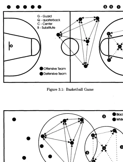
3.1 Analogy with the Basketball Game

Please notice that if it were possible to watch a basketball game from above we could see there is an analogy with ad-hoc networks, that is because the mobility of the players, the interchange of the ball within them and the score. For example lets see Figure 3.1, in this case we have a typical basketball game, the black team wants to score, and the white team defends its basket. Each player can communicate with each other or of the white or black team.

Now, in Figure 3.2, we show a cluster topology for ad hoc networks. We notice a similarity between the two figures. For this, we can introduce a new cluster algorithm that has some characteristics of the game of basketball based on the teamwork of the players. Next, we explain this analogy an the meaning in our model.

G ­ Guard Q ­ quarterback C ­ Center B ­ Substitute

) Offensive Team > Defensive Team

Figure 3.1: Basketball Game

Black Cluster White Cluster

G ­ Ordinary node Q ­ Clusterhead C­Gateway B ­ Substitute

Basketball game (definition):

Basketball is played by two (2) teams of five (5) players each. The aim of each team is to score in the opponents' basket and to prevent the other team from scoring. Basket-ball is controlled by officials, table officials and a commissioner.

Tag Clustering:

A cluster will be conformed by a team of a number of nodes each. The aim of each clus-ter is to generate routes to inclus-terchange packets of information between the nodes. Each equipment will be conformed by clusterhead (quarterback), ordinary nodes (guards and benchs) and Gateways (Centers).

Basketball game (players):

Five (5) players from each team shall be on the court during playing time and may be substituted. One quarterback, two guards and two centers.

The quarterback is who organized the play, it's faster than the other players and passes the ball in several occasions. The guard is who score the majority of the points. The center is the tallest player and he takes the defensive rebounds.

A substitute becomes a player and a player becomes a substitute when: The offi-cial beckons the substitute to enter the playing court. During a charged time-out or an interval of play, a substitute requests the substitution to the scorekeeper.

We take the statistics1 _{of the best player of all the times in the NBA as we show}

in Figure 3.3

Tag Clustering:

The Clusterhead (quarterback) will be in charge to direct the team. Within the statis-tics it will be that node that has the greater number of participation to reveal packtes to another node destination (APG). Its trustworthiness in the connection and its prox-imity with other clusters will be greater than the guards but smaller than the center's.

J_{PPG= Points per Game, RPG= Rebound per Game, APG= Assists per Game.}

Position: Center Height: 2.16 m Weight: 147.4 Kg Shaquilie O'Neal STATISTICS PPG 26,7 RPG 12 APG 2.8 Position: Guard Height: 2.01 m Weight: 97.97 Kg Michael Jordan STATISTICS PPG 30.1 RPG 6.2 APG 5.3 Position: Guard Height: 2.03 m Weight: 103,4 Kg Scottie Pippen STATISTICS PPG 16.1 RPG 6.40 APG 5,2 Position: Quarter Height. 2.10 m Weight: 115.6 Kg Earvin Johnson STATISTICS PPG 19.5 RPG 7.? APG 11.2 Position: Center Height: 2.01 m Weight: 114.3 Kg Charles Berkley STATISTICS PPG 22.1 RPG 11.7 APG 3.9

It will be in charge to take the statistics of the team (if sizing is not used). It will be labeled with MX where X is the number of the cluster to which it belongs.

The guards will be those nodes that have the greater number of packets transmitted by time unit (PPG). Their trustworthiness in the connection and its proximity with other clusters will be similar. They will be labeled with GX where X is the number of the equipment to which they belongs.

The centers will be those nodes that have the greater number of rescue of a route, i.e., if some route is broken during the transmission, these nodes participate to rescue the transmission of the package (RPG). They have a trustworthiness in the connection and a proximity with other clusters much greater than the clusterhead and the guards. They will be labeled with CX where X is the number of the cluster to which they belongs.

The substitute will be conformed by those nodes that have two or more different con-nections with clusters, will be up to three jumps of distance from the gateway and can belong to two or more clusters, i.e., we consider overlapped clusters. The decision to belong to a cluster or to enter one of the clusters will the be responsibility of the clusterhead. They will be labeled with BX, where X is the number of the cluster to which it belongs. Also we can have substitutes in the ordinary nodes for the centers and for the clusterhead, we do not consider substitutes for the guards.

Basketball game (fouls):

During a game in which ten (10) players are moving at high speed in a limited space, personal contact cannot be avoided. A foul is an infraction of the rules concerning ille-gal personal contact with an opponent and/or unsportsmanlike behavior. Any number of fouls may be called against a team. Irrespective of the penalty, each foul shall be charged, entered on the score sheet against the offender and penalized accordingly. If a player commits five fouls is expelled from the game.

Tag Clustering:

Fouls are the routes that have disappeared by the birth or death of a node, by a coverage anomaly in the transmission of a node, labeled interchange of or some other situation that affects a trajectory of communication between the nodes. When accu-mulating 5 fouls the node will be labeled like nonreliable and a timer will be start to

count for 5 minutes, and until the term of 5 minutes it could again be considered for the generation of routes. It will be labeled with FX where X is the number of the cluster to which it belongs.

The markers of fouls of the nodes, must be to available to the nodes to generate reli-able routes. When accumulating 5 fouls a node will be labeled like nonrelireli-able. When accumulating 5 foules by equipment, is to say that the equipment are accumulated 25 fouls (each one of the 5 members has fouls in its account) the equipment is not reliable and cluster will not be taken into account for outer routes to the equipment including all the cluster.

The death of a node is a random event when, the node is no longer present in the network, or in the case where a node due to mobility lies outside a cluster which used to be part of. Also, the low trustworthiness in the connection causes a node to die. The clusterhead registers this information in the statistics. A dead node will be labeled with DX, where X is the number of the cluster to which it belongs.

The dead time is the calculation of the inactivity of some node within a cluster, i.e., the node does not participate when commanding messages or like part of a route. The dead times will be defined within the tables of statistics.

The birth of a node is a random event when a new node appears within a cluster and it will have to identify itself with the clusterhead and after passing the 5 minutes labeled as unreliable, the corresponding label will be granted to him. It will be labeled with NX, where X is the number of the equipment to which it belongs.

We show the tag of every node in Figure 3.4, in the next section we talk about the statistics used in the tag of the nodes.

3.2 Statistics in the Tag Clustering

Each node has a routing table that indicates the possible trajectories, the statis-tics and the label of each attainable node. The control table contains all the located statistics of clusters within its coverage area.

.Team­Cluster 1

Team­Cluster 3

Team­Cluster 2

GX ­ Guard node MX ­ Clusterhead CX ­ Center node BX ­ Gateway DX ­ Dead node NX ­ New node

Figure 3.4: Ideal Tag Clusterig

the nodes try to diminish this aspect.

The control table will be part of the routing table, i.e., within the table, we find measures of efficiency of each node in the cluster, these measures will be handled by the clusterhead. The clusterhead has knowledge of all the nodes in the cluster, so that, it can make a decision about which route is more efficient to be followed.

The statistics must be provided by the clusterhead and must be available to the nodes for routing decisions. Within the cluster, routes must have clearly visible statistics for all the involved nodes in the network, including others from different clusters. The statistics must indicate, at least:

• Identification of the cluster.

• Trustworthiness in the connection and proximity to other clusters.

• Identification of the nodes who participate within the cluster.

• Identification of the nodes that have gateways (centers) as well as the neighboring clusters that can be reached.

• Accumulated fouls by each node.

• Accumulated fouls by each cluster.

• Packets transmitted by time unit (PPG) by node.

• Number of participation to reveal packets to another node destination (APG).

• Rescue of routes (RPG) by each node.

• The routes marked by each cluster and, preferably the routes in which each node participates.

• Active routes with time label.

3.3 Tag clustering Algorithm

Tag Clustering Algorithm is a clustering algorithm designed to use in mobile ad hoc networks. The algorithm divides the nodes of the ad hoc network into a number of overlapping or disjoint 1-hop- diameter clusters in a distributed manner. A clus-ter head (quarclus-ter) is elected for each clusclus-ter to maintain clusclus-ter statistic information. Inter-cluster routes are discovered dynamically using the cluster player's tags informa-tion kept at each cluster head. By clustering nodes into teams, the algorithm efficiently minimizes the number of gateways (centers) and broken routes could be repaired locally without rediscovery with the substitutes using cooperative work. The objective of the tag clustering algorithm is to find a feasible interconnected set of clusters covering the entire node population.

Tag clustering algorithm has two logical stages: first, the formation of clusters and, second, the tagging of the nodes. Each node performs the steps of the algorithm based on local information. Thus the algorithm is distributed. Some exchanges of messages are required in this algorithm. Once we have the completion of the algorithm the net-work is organized into clusters and each node ends up assuming one of theses roles; it may remain an ordinary node (guards), it may become a gateway node (centers), it may become a substitute (quarter substitute or center subsitutute), or it may become the cluster head (quarter) node position. The significance of these roles will become apparent as the algorithm is described.

We assume that each node in the network uses a Global Positioning System or has the position information available and each node is identified by a unique integer from I to N and is allowed to transmit control messages related to the algorithm.

data structures: two lists called, respectively, SINGLENODE, NEIGHNODES, two matrix called CONNECTIVITY and DISTANCES, a variable POSITION, and an in-dicator named NODESTATUS. These data structures are updated routinely as control messages are received from other nodes. We first describe what these data structures represent.

The CONNECTIVITY matrix has binary entries. A value of 1 in the (i,j)th

posi-tion indicates the existence of a link between nodes i and j, and a value of Q the lack

of one. Thus, the ith row of the matrix indicates the connectivities of the ith node. It is possible that at the location of node i several rows of the matrix remain unfilled due

to the lack of knowledge about the connectivities at distant locations in the network. The variable POSITION gives us the position in the coordinates (/i, k) of the node and

we can calculate the distances between the nodes using:

(3.1)

After this, we have the DISTANCES matrix whose entries are obteined by (3.1). Thus, the (i, j)ih. element of the matrix indicates the distances between the ith node and the jih. node.

The variable QUARTER designates the identity of the node that is assigned to be the clusterhead for a given node. The NODESTATUS indicator takes on one of for values, GUARD, CENTER, SUBSTITUTECENTER, SUBSTITUTEQUARTER or QUAR-TER to specify the role assumed by a given node. The NEIGHNODES list includes all neighboring nodes that a node can hear. The SINGLENODE list records those nodes that are not connected to a any node.

In the beginning the algorithm proceeds as follows.

Nodes broadcasts their position and compute the distances between them.

Node i broadcasts the identities of the nodes it has heard from 1 hop, during the

earlier broadcast (POSITION and DISTANCES). Thus, node i also receives partial

connectivity information of the nodes that it can hear. So at the end of this frame, node i has filled in some of the entries of its connectivity matrix. In particular, it can

fill in elements (i, j) of the ith row that satisfy j > i. The element (i, j) is set equal to

1 if node i hears from node j and node i appears in the NEIGHNODES list broadcast

by node j.

Node i can perform the first stage of the tag clustering algorithm to form clusters and the second stage to determine the NODESTATUS, using its row connectivity informa-tion. We see in the Figure 3.5 and 3.6 the two stages of the tag clustering algorithm. We use the rule that the node with the maximum number of NEIGHNODES among a group of nodes is the first candidate to claim QUARTER status (clusterhead). Thus, node i first checks its connectivity row. If there is two o more nodes with the maximum NEIGHNODES, we use the rule that the node with the lowest identity number among a group of nodes is the first candidate to claim QUARTER status. The other nodes will be substitutes of the cluster head (SUBSTITUTEQUARTER)

Single / Yet/Node without

Nodes with maximun number of neighbors

Intersection of sets of neighbors of tentative

clusterhead

/ empty

/­

1 _No

/Intersection 'Xjfes^y CkntBihead (Quarter)

/ Fight for be / dusterhead /

x _{Node ID Fight  \ Y e s / ^}

splusterhead = n*!/ / (Quarter)

Clusterhead / (Quarter) / Substitute /

I Ordinary nodes | (players) = j Neighbors of

\ Clusterhead

Figure 3.5: Formation of clusters in tag clustering algorithm

Number of cluster Single node Qustertiead (quarter) SubsttuteofOustofhoad

Gatoways(ceoter)

Sutattute of Gateways Guard*

c

Compute distance*

between the

dustertieads and

each on of the nodes

of 8ie gate ways sets

Chapter 4

Performance Evaluation

A simulator model was constructed to provide examples of ad hoc networks using the tag clustering algorithm just described, and to depict the resulting organization. In this chapter, we show selected samples of simulation outputs that illustrate several of the possibilities that may arise and the corresponding action by the algorithm. The input parameters for the simulator are the number of nodes, the communication range, a seed number for generating random node positions and the maximum spatial size of the network.

We generate a random network whose nodes are randomly distributed according to a spatial Poisson point process of density A users per square meters. We simulate a system of n nodes on a 1000 x 1000 square meters. The nodes could move in all

possi-ble directions with speed varying uniformly between 0 to a maximum value (m/s). In our simulation experiments, n was varied between 50 and 200, and the nodes moved

randomly in all possible directions.

We compare the performance of tag clustering algorithm with seven performance met-rics: (i) the number of clusterheads, (ii) the number of Single nodes, (iii) the number of gateways, (iv) the number of ordinary nodes, (v) the number of clusterhead substitutes, (vi) the number of gateways substitutes, and (vii) reachable clusters. The number of clusterheads in the network defines the dominant set. These parameters are studied for varying number of nodes (n) in the system and maximum displacement.

In the first simulation (it is our most important simulation) the nodes were then al-lowed to move at random in any direction at a speed no greater than 10 m/s. The simulation ran for 3600 seconds, and the network was sampled every second. At each sample time the proposed Tag Clustering Algorithm was run to determine clusterheads and there associated nodes (ordinary nodes, gateways, clusterhead substitute and gate-way substitute). For every simulation run the performance metrics mentioned before were measured for the entire 3600 second of simulation. Some of the more noteworthy simulation performance metrics measured are shown in Table 4.1. These performance

metrics provides a basis for evaluating the performance of the proposed algorithm.

Table 4.1: Static Results for 3600 seconds

Average Single nodes Clusterhead Gateways Clusterhead substitute Gateways substitute Ordinary nodes Reachable clusters Nodes per cluster Gateways per cluster Guards per cluster

Gateways substitute per cluster Clusterhead substitute per cluster

Communication radio Maximum Minimum 5 25 58 13 30 52 3.4375 8.1667 2.8421 4.3333 1.8125 0.7059 0 12 19 0 3 7 1.25 4 1.1875 0.3182 0.1429 0 of 150m Mean 0.9172 18.6722 37.3689 3.5347 13.9661 25.5408 2.3096 5.3562 2.0056 1.4006 0.7579 0.1922

The objectives when designing the clustering algorithm were the following: The algorithm must be distributed, since every node in the network only has local knowl-edge. The algorithm should scale well as the size of the network increases. The created clusters should be reasonably efficient, that is, the selected clusterheads should cover a large number of nodes. If the clustering structure becomes too complex (too many clusters), the number of messages needed to maintain the routing structure would cause congestion in the network.

In the following sections we compare the algorithm in different situations varying the number of nodes, the communication range and the speed of the mobility.

4.1 Proposed Scenarios

In this section we propose two types of scenarios where we apply the concepts described before. The scenarios are

• Scenario 2, in this scenario, we compare the cluster performance measures, when we vary the velocity of the nodes, the total number of nodes and the communi-cations range.

4.1.1 Scenario 1

This scenario consists of static simulations of the algorithm, it is important to say that in every slot of time, we generate random nodes with a spatial Poisson distribu-tion, with no mobility; the objective is to observe the behavior to drastic changes of the topology of the ad-hoc network. The simulations are made in 50 slots of time, at each sample time the proposed Tag Clustering Algorithm was run to determine clus-terheads and there associated nodes (ordinary nodes, gateways, clusterhead substitute and gateway substitute). Varying the number of nodes in the system, we tried to cover low density, medium density and high density networks. The low density is conformed by an approximated number of 50 nodes, we deduced that we will find a considerable number of single nodes and a low number of clusters, with this the algorithm will be exposed to low communication.The medium density is conformed by an approximated number of 100 nodes, this node density is considered stable in the communication and with a low number of single nodes. We chose to vary the communication range. At the beginning the range is of 150 m and its behavior is observed, then we change the range to 200 m and we observe the changes in the performance parameters. The high density is conformed by an approximated number of 200 nodes, where we see that the number of single nodes will be almost null and the number of clusters will be increased, with this we want to observe the behavior of the tag clustering algorithm in high density and check the growth of the number of clusters.

Table 4.2 shows the parameters of performance for the 3 types of densities. We ob-served that the number of single nodes is greater in the low density and is almost null for high density. The number of clusterheads is equal to the number of clusters since we only have one clusterhead per cluster, we observe that an approximated increase of 30 percent of the number of clusters when we increase the density and this indicates a stability of the algorithm because the number of clusters is not increased considerably when we have high density. The number of gateways indicates the possibilities of con-nection with others clusters, since it had been predicted in low density we do not have a considerable connection, and in the high density the connection grows considerably, allowing to find routes between clusters. The substitutes indicate the possibilities of saving routes in case of the death of some of the clusterhead or gateway, the most important point is the increase in the number of gateway substitutes in high density this provides communications to almost all the nodes in the system. In order to deter-mine certain form of robustness in the algorithm, we propose a performance parameter

based on the average of reachable clusters for this we considers the average of reachable clusters per clusters and the average of this in the 50 time slot, it is observed that the number of reachable clusters for different densities increases when we increase the density.

Table 4.2: Static Results for different node density

Average Single nodes Clusterhead Gateways Clusterhead substitute Gateways substitute Ordinary nodes Reachable clusters Communication range 50 nodes 100 nodes

3.08 15.6 10.36 3.48 0.82 15.72 1.228528653 0.76 20.64 29.36 4.46 5.52 29.86 1.940592021 of 150m 200 nodes 0.04 26 72.22 5.22 43.8 54.08 3.518796012

Figure 4.1 shows the CDP of single nodes for the 3 user densities, we observed a greater number of jumps in the distribution for low density that indicates a greater number of single nodes, with 9 single nodes in the worse case. For medium density, we have 4 single nodes in the worst case, and for high density, we have 1 single node. Figure 4.2 shows the probability of having single nodes and a average of clusterhead/ordinary nodes in the system, it is easy to observe the decay of the probabilities as we increase the density.

We can observe the diminution in the average of clusterhead/ordinary nodes if we increase the density, in Figure 4.1 since the number of ordinary nodes almost increases to the double when the density grows, but the number of clusterhead is increased in a 30 percent. On the other hand we have Figure 4.3 that shows the possibility of rescuing a gatewaey in case that it dies, with this factor has trustworthiness in the different con-nections between clusters. We observed the increase when we increment the densities.

1

0.9

0.8

0.7

x"

fi o

n 1 •

© '

— 1 | 1 I 1 I 1

= X I ; ^ J O

v ; _- ; _'••

v • ; _'•

: : :

: : : :

! 1 i i i -0- 50 nodes ! ! i ; : -X- 100 nodes | i i ; I e 200 nodes

-i -i -i -i -i -i -i

8 9

Figure 4.1: Empirical CDF for Single Nodes

i­

OJD

00

0,4

02-0

.4Clusteihead/

OnJnay nodes

­•Single Nodes

50 100 200 100

200m

Figure 4.2: Connectivity Weakness Probability

0.7

0.6

0.5

. 0.4

0.3

0.2

0.1

50 100

User Density

100

200m 200

Figure 4.3: Connectivity Probability

We found an acceptable behavior of the algorithm for scenario 1, now we will observe the behavior when we varied the radius of communication to 200 ms for the medium density, in the Table 4.3 we observed the performance metrics.

Figures 4.2 to 4.4 also show the behavior for the communication range of 200 m. We can observed a similar behavior between high density and the communication range of 200 m. The communication range will be a control variable to increase the robustness when it will necessary. In the others metrics we have almost the same behavior.

The service provides could change this control variable, sending a message to the quar-ter to increase the communication range, if the number of robustness is less than 2. In a real ad-hoc network environment will be have other variables that we do not take to consideration because it will be part of a further work.

4.1.2 Scenario 2

3.5

2 5

1.5

50 100

User Density

100

200m 200

Figure 4.4: Reachable clusters

Table 4.3: Static Results for different communication range Communication range of 150m and 200m Average

Single nodes Clusterhead Gateways

Clusterhead substitute Gateways substitute Ordinary nodes Reachable clusters

100 nodes (150m) 0.76

20.64 29.36 4.46 5.52 29.86 1.940592021

100 nodes (200m) 0.04

14.02 30.68 3.22 13.96 28.68 2.750901574

behavior of the topology of the network when we have movement. The simulations are made in 50 slots of time, at each sample time the proposed Tag Clustering Algorithm was run to determine clusterheads and there associated nodes.We will use the same considerations of densities that we took for scenario 1. the difference will be that we will have mobility with variations of speed from 3 to 10 m/s).

In the Table 4.4 we have the results obtained for the different densities, we observed similar behavior to those of scene 1 in the parameters of single nodes, clusterhead, gateways, gateways substitute and ordinary nodes. Figure 4.5 shows to the CDF for single nodes showing again that with low density obtains the greater number of single nodes, with 5 for the worst cases. For medium density we have 2 as worst case and for high density we do not have single nodes.

Table 4.4: Movement Results for different node density (speed 3 to 10 m/s)

Average Single nodes Clusterhead Gateways Communic 50 nodes 2.58 12,8 12.72 Clusterhead substitute i 2.8 Gateways substitute Ordinary nodes Reachable clusters 2.24 16.86 1.210149374 2 ation range 100 nodes 0.7 18.86 36.98 2.66 14.88 25.92 .345787785

of 150m 200 nodes 0 22.7 70 4.66 60.84 41.8 3.471350029

Figure 4.6 shows the probability of existence of single nodes, where we found a decay again as we increased the densities; in these graphs we can observe different additional parameters from the 3 densities, among them we have 100 nodes in 3600 seconds of simulation, with different speed and different radius from cover. The first parameter will give us the behavior in large slot of time and show that the algorithm is stable for all the times; the second parameter will give us the stability of the algorithm for high speeds (23 to 30 m/s), but is know that a ad hoc network will not work in high speed. Ahead we will discuss the results obtained for these new parameters.

0?

A -I

n

S>

!

1

4- '

i 1.5 :

!

!

fS

S*1 ^

i

2 2.5 : X

' ! f

; : /*-\ 0 ' ^

: : |

-Q- 50 nodes -X- 100 nodes

o 200 nodes

5 3.5 4 4.5 S

Figure 4.5: Empirical CDF for Single Nodes

oa-00

02-ClusterheacV Otdnoy nodes

\ angle nodes_%

» i

SO lOOlhf 100 100200m 200

Figure 4.6: Connectivity Weakness Probability

0.9

0.8

0.7

0.6

0.5

0.4

0.3

0.2

0.1

50 lOOlhr )00 lOOvaaciJO

User Density 100200m 200

Figure 4.7: Connectivity Probability

with this factor has trustworthiness in the different connections between clusters. We observed the increase when we increment the densities.

Figure 4.8 shows the robustness to us of the algorithm for different densities, we concluded that a robustness of 3 is acceptable for tag clustering in movement, because in high density the robustness is greater to 3,5 and with medium density increasing the radius of communication is greater to 3 reaching an acceptable communication between clusters.

We observer closest values between scenario 1 and 2, and the same behavior in the figures, this will help us to get a good conclusion of the performance of the tag cluster-ing algorithm.

3.5

2.5

1.5

50 _lOOlhr 100 100v«23a3<>

User Density 100200m 200

Figure 4.8: Reachable clusters

will be have other variables that we do not take to consideration because it will be part of a further work.

We found an acceptable behavior of the algorithm for scenario 2 now we can use tag clustering for routing packets between the nodes, now we will observe the behavior when we find the route between two nodes using dijkstra algorithm and a approxima-tion of the tag routing algorithm. We will proposed the general idea for the routing in tag clustering, the performance of this will be part of further work.

4.2 Finding the Shortest Path

The general idea for the tag routing algorithm is that the nodes that belongs a cluster has the routing table of the cluster. The clusterhead will have the statistic table and substitute table. The gateway will have the cluster neighbor table.

If a node want to send a packet to another node, first they have to send it to the clusterhead, the clusterhead taking account the statistic will decide the best route; if

Table 4.5: Movement Results for different node density and speed Average Single nodes Clusterhead Gateway Clusterhead substitute Gateway substitute Ordinary nodes Reachable clusters

Communication range of 150m 100 nodes(3-10 m/s) 100 nodes(23-30 m/s) 100

0.7 18.86 36.98 2.66 14.88 25.92 2.345787785 1.18 17.98 36.52 3.2 15.6 25.52 2.351151162 3 nodes(200 m) 0.46 12.86 36.24 2.12 26.5 21.82 .287317493

the destination node belongs to the cluster the clusterhead will send the packet, if not it will send the information to the gateway. The gateway will check in there cluster neighbor table the gateway of the other clusters, and it will send it to them. Now the gateway will send the the packet to the clusterhead and will use the same idea described before.

In Figure 4.9 show the shortest path using dijkstra algorithm for a 100 node density and 200 m of communication range. Figure 4.10 show the shortest path using dijkstra algorithm with the same node density and network topology. With a communication range of 150 m. Figure 4.11 show tag routing in the same node density and network topology using tag clustering algorithm. With a communication range of 150m. In all the cases node 92 wants to send a data packets to node 5.

4.3 Communication Overhead

Tag clustering algorithm is a hybrid algorithm that use concepts of the Lowest-ID and the Highest-connectivity clustering algorithms, for this the communication overhead will be the same that them. Node mobility can cause topology changes (link/cluster additions/deletions) to propagate up to any level. Despite this complica-tion, John Sucec and Ivan Marsic [15] derived the following break-downs of the control overhead. The values are expressed as packet transmissions per node per second unless otherwise specified.

• ^Hello = 0(1) - "Hello" protocol

1000-

900-

800-

700-

600-

500-

400-

300-

200-

100-100 200 300 400 500 600 700 800 900 1000

Figure 4.9: Shortest Path communication range 200m without clustering

0ACQ = Olog(N) - acquisition of local data when node migrates from one cluster

to another.

^Flood = Olog(N) - flooding of cluster topology updates to cluster members.

<^Reg = (N) - location registration events.

^Handoff = 0log*(N) - handoff or transfer of location management data.

= 0(ti) - query events.

• ^Ctrl-Header = Olog(N) - bits per control message datagram - addressing

infor-mation required in datagram headers.

In summary, the total communication overhead in such a hierarchical routing protocol is 9log2(N) packet transmissions per node per second and Olog3(N) bits per

node per second, assuming that the node density, mobility, and traffic load remain constant. This is a substantial (exponential) improvement over the linear costs of routing in at networks. We propose in the chapter 5 an analysis of the overhead produced by the statistics.

1000

900-

800-

700--600h

500r

400h

300 h

200h

100:-I

800 I

900

0 100 200 300 400 500 600 700 800 900 1000

Figure 4.10: Shortest Path communication range 150m without clustering

lOOOr

900800

-

700-200 300 400 500 600 700 800 900 1000

4.4 Tag Clustering Algorithm vs Different

Cluster-ing Algorithms.

We cannot have a comparison between tag clustring and different clustering algo-rithms becouse the main idea of tag clustering is the cooperative work, as we explain in the chapter 2, that is a new topic in the related to topology generation, organization and maintenance. For this in Table 4.6 we show in a general manner the different clustering algorithms [8].

Table 4.6: Summary of Different Clustering Algorithms

Algorithm Lowest-ID (LCA2) Highest-connectivity Tag clustering Max-min D-cluster Hierarchical Adaptive clusters Properties Clusterhead selection

based on node ID. Clusterhead is directly linked to any other node

in the cluster. Clusterhead selection based on higheset degree,

otherwise same as LCA2 Clusterhead selection based on highest degree,

if we have nodes with the same highest degree

the node with the min ID will be the CH.

Cluster radius d,

where d is a constant. No fixed diameter of each cluster. Cluster size < Jfc,2Jfc-l >,

where k is a

constant. Created clusters

should be connected in time

t with probability

a

Complexity Constante time complexity, message

complexity increase with denseness of

graphs Same as LCA2 Same as LCA2

0(d) time and clusters Time complexity

0(E) Undefined.

Strengths Fast and simple

algorithm. Relatively stable

clusters. The nodes with highest degree are good candidates for

clusterheads Cooperative

work. Taggin of the

nodes. Large and stable Guaranteed upper and lower bound on

cluster size. a and t can be

varied in order to adapt to different mobility rates. Weaknesses Small clusters. Some clusterheads likely to ramian for

long tune. Very unstable

clusters. FVirther work

High number of messages sent. Slow algorithm. Cluster radius can

be up to k.

algorithm Difficult to predict

future connectivity.