Incorporating boundary conditions in a stochastic volatility model for the numerical approximation of bond prices

DOI: xxx/xxxx

SPECIAL ISSUE PAPER

Incorporating boundary conditions in a stochastic volatility model

for the numerical approximation of bond prices

Lourdes Gómez-Valle

_{| Miguel Ángel López-Marcos}

_{| Julia Martínez-Rodríguez}

1_{Departamento de Economía Aplicada e}

IMUVA, Facultad de Ciencias Económicas y Empresariales, Universidad de Valladolid, Spain

2_{Departamento de Matemática Aplicada e}

IMUVA, Facultad de Ciencias, Universidad de Valladolid, Spain

Correspondence

Julia Martínez-Rodríguez, Departamento de Economía Aplicada e IMUVA, Facultad de Ciencias Económicas y Empresariales, Universidad de Valladolid, Spain. Email: [email protected]

MSC Classification: 65M06, 91G30.

Summary

In this paper, we consider a two-factor interest rate model with stochastic volatility

and we assume that the instantaneous interest rate follows a jump-diffusion process.

In this kind of problems, a two-dimensional partial integro-differential equation is

derived for the values of zero-coupon bonds. To apply standard numerical methods to

this equation, it is customary to consider a bounded domain and incorporate suitable

boundary conditions. However, for these two-dimensional interest rate models there

are not well-known boundary conditions, unlike option models. Here, in order to

approximate bond prices we propose new artificial boundary conditions which

main-tain the discount function property of the zero-coupon bond price. Then, we illustrate

the numerical approximation of the corresponding boundary value problem by means

of an Alternative Direction Implicit method which has been already applied for

pric-ing options. We test these boundary conditions with several interest rate pricpric-ing

models.

KEYWORDS:

interest rate model, zero-coupon bonds, jump-diffusion stochastic processes, stochastic volatility, risk-neutral measure, boundary conditions, Alternative Direction Implicit methods

1

INTRODUCTION

The term structure of interest rates is one of the most important topics in the study of economics and finance. On the one hand, it provides useful information concerning market expectations of future real activity and inflation, that is, the conventional final targets of monetary policy. On the other hand, it is a very important subject in pricing models, risk management, hedging and arbitrage. In fact, many researches focus on the dynamic models of the term structure.

Traditionally, interest rates are assumed to move continuously and, in the literature, diffusion processes are used to model their

behaviour10,27_{. However, different market phenomena, such as shocks or surprises, provide unexpected jumps in the interest}

rates, as a result of this, the most realistic models use jump-diffusion stochastic processes to model interest rates11,22_{. Moreover,}

pricing and hedging with jump-diffusion models is crucial, since ignoring jumps can produce hedging and pricing risk23_.

It is widely known that one-factor interest rate models are very attractive for practitioners because of its simplicity and com-putational convenience. However, these models have also unrealistic properties. Firstly, they cannot generate all the yield curve shapes and changes that we can find in the markets. Secondly, the changes over infinitesimal periods of any two interest-rate

dependent prices will be perfectly correlated. Finally, as Hong and Li 17 _{show, none of their analyzed one-factor models}

ade-quately captures the interest rate dynamics. Therefore, at least two factors are necessary in order to properly model the term

0_{Abbreviations:ADI method, Alternative Direction Implicit method; PIDE, partial integro-differential equation; HV method, Hundsdorfer-Verwer method; MHV}

structure of interest rates. In fact, the number of factors must be a compromise between an efficient numerical implementation and the capability of the model to fit the experimental data.

In the literature, the different functions describing the stochastic variables of the model are usually chosen to be affine: the aim

is to obtain a pricing problem with a feasible closed-form solution. However, when more realistic functions are considered15_,

a feasible expression of the solution is not achieved. Then, numerical methods should be used to approximate the solution. In such a case, we can underline two techniques. On the one hand, as zero-coupon bond prices can be obtained as expectations, the Monte Carlo approach provides a valuable tool: by the law of large numbers, the integrals that describe the expected value of the underlying random variables can be approximated by means of independent generated paths of such random variables. The Monte Carlo method is simple, flexible, and can handle multiple sources of uncertainty. However, this technique provides low accuracy approximations with a very high computational cost. On the other hand, we can also use numerical methods based on the discretization of the differential equation in order to approximate its solution12_{. More specifically, if the model involves a}

jump-diffusion process, we have to deal with a partial integro-differential equation with a final condition.

From a numerical point of view, in order to discretize the problem, first of all a bounded domain for the state variables must be considered. Hence, suitable boundary conditions must be established. In bond pricing literature, only one-factor interest rate models are usually investigated. In this case, the restriction of the equation when the interest rate is zero and an artificial Dirichlet condition based on the behaviour of the solution for the maximum interest rate are incorporated5,8,13_{. However, there is a lack}

of investigation when the number of state variables is greater than one.

If we analyse other financial derivatives, such as options, finite difference schemes are usually considered for pricing European and barrier options in jump-diffusion models7_{. For the multifactor case, first, a transformation in the partial integro-differential}

equation is usually made to eliminate the mixed derivative term. Then, several suitable methods are considered with very well-known and established boundary conditions14,19,20_{. However, this is not applicable to general interest rate models.}

In this paper, we focus on the approximation of zero-coupon bond prices in two-factor jump-diffusion models where the state variables are the instantaneous interest rate and the volatility. The numerical approach requires the discretization of a multidimensional problem involving a partial integro-differential equation: so we have to discretize some differential terms and a nonlocal integral term. As the problem has only a final condition, we introduce a bounded domain for the state variables. The main difficulty is to fix appropriate boundary conditions compatible with the model. Here we propose such restrictions taking into account the discount function property of the zero-coupon bond price. We illustrate the implementation of a numerical

method for the proposed boundary value problem by using a well-known ADI method: the Hundsdorfer-Verwer scheme20_.

The paper is organized as follows. Section 2 describes a two-factor jump-diffusion model with stochastic volatility to price interest rate derivatives. In Section 3, we propose suitable boundary conditions for the numerical approximation of this kind of models, and we implement an ADI method for the emerging boundary value problem. In Section 4, we validate the numerical technique by means of the approximation of the yield curves in two well-known term structure models. Section 5 collects the conclusions.

2

THE JUMP-DIFFUSION MODEL

We present a two-factor jump-diffusion model for pricing zero-coupon bonds. Define(Ω,,{𝑡}𝑡≥0,)as a complete filtered

probability space which satisfies the usual conditions, where{𝑡}𝑡≥0is a filtration2,6,25. We assume that the state variables are

the dynamics of the instantaneous interest rate,𝑟, and the volatility,𝑉. In order to take into account the abrupt changes of the interest rates in the markets, we consider that such interest rate follows a jump-diffusion stochastic process. We suppose that the volatility is a diffusion process1_,16_{:𝑟is right-continuous (cadlag}6_{) and we denote the left limit𝑟(𝑡−) = lim}

𝑧↑𝑡𝑟(𝑧)(however, for

notational clarity the pre-jump values𝑟(𝑡−)will be added only when necessary to avoid confusion and otherwise, they will be

assumed implied). Thus, these factors follow this joint stochastic process:

𝑟(𝑡) = 𝑟(0) +

𝑡

∫

0

𝜇𝑟(𝑟(𝑧), 𝑉(𝑧))𝑑𝑧+ 𝑡

∫

0

𝑉(𝑧)𝑑𝑊𝑟(𝑧) + 𝑡

∫

0

𝑐(𝑟(𝑧−), 𝑉(𝑧))𝑑𝑞(𝑧), (1)

𝑉(𝑡) = 𝑉(0) +

𝑡

∫

0

𝜇_𝑉(𝑟(𝑧), 𝑉(𝑧))𝑑𝑧+

𝑡

∫

0

where𝜇_𝑟and𝜇_𝑉 are the drifts and𝜎_𝑉 the volatility of the implied volatility process. Moreover,𝑊_𝑟and𝑊_𝑉 are Wiener processes, and the impact of the jump is given by function𝑐and the compound Poisson process𝑞(𝑡) =∑_𝑖𝑁₌₁(𝑡)𝑋𝑖, with jump times(𝜏𝑖)𝑖≥1.

The Poisson process is represented by𝑁(𝑡)with intensity𝜆(𝑟, 𝑉); and𝑋₁, 𝑋₂,…is a sequence of identically distributed random variables with a Normal probability distributionΠ,_(0, 𝜎𝑋). We assume that𝑊𝑟,𝑊𝑉 are correlated with

[𝑊_𝑟, 𝑊_𝑉](𝑡) =𝜌𝑡,

but the jump size distribution and both standard Brownian motions are independent of𝑁. We also assume that the jump

mag-nitude and jump arrival times are uncorrelated with the diffusion parts of the processes. Lastly, we suppose that the functions

𝜇_𝑟, 𝜇_𝑉, 𝜎_𝑉, 𝜆andΠsatisfy suitable regularity conditions3,24_.

As in previous works16_{, we assume that the market is arbitrage-free. Then, there exists an equivalent martingale measure,}

-measure, which is known as the risk-neutral measure (see the extended Girsanov-type measure transformation4,26_{). The state}

variables of the model (1)-(2) under the risk-neutral measure are as follows:

𝑟(𝑡) = 𝑟(0) +

𝑡 ∫ 0 𝜇_𝑟(𝑟(𝑧), 𝑉(𝑧))𝑑𝑧+ 𝑡 ∫ 0 𝑉(𝑧)𝑑𝑊_𝑟(𝑧) + 𝑡 ∫ 0

𝑐(𝑟(𝑧−), 𝑉(𝑧))𝑑 ̃𝑞(𝑧), (3)

𝑉(𝑡) = 𝑉(0) +

𝑡 ∫ 0 𝜇_𝑉(𝑟(𝑧), 𝑉(𝑧))𝑑𝑧+ 𝑡 ∫ 0

𝜎_𝑉(𝑟(𝑧), 𝑉(𝑧))𝑑𝑊_𝑉(𝑧), (4)

where𝜇

𝑟 =𝜇𝑟−𝑉 𝜃𝑊𝑟,𝜇𝑉 =𝜇𝑉 −𝜎𝑉𝜃𝑊𝑉. The Wiener processes under-measure are𝑊𝑟and𝑊



𝑉 , and[𝑊𝑟, 𝑊



𝑉 ](𝑡) =𝜌𝑡. The market prices of risk associated to𝑊_𝑟and𝑊_𝑉 Wiener processes are𝜃𝑊𝑟_{(𝑟, 𝑉)and𝜃}𝑊𝑉_{(𝑟, 𝑉), respectively. The compensated}

compound Poisson process under-measure is𝑞̃(𝑡) =∑𝑁_𝑖=1(𝑡)𝑋_𝑖−𝜆𝑡𝐸_𝑋[𝑋₁], and𝜆(𝑟, 𝑉)is the intensity of the Poisson process𝑁(𝑡). Finally, we consider the function𝑐(𝑟, 𝑉) = 1in (3).

A zero-coupon bond price at time𝑡, with maturity time𝑇,𝑡≤𝑇, under the above assumptions, is

𝑝(𝑡, 𝑟, 𝑉;𝑇) =𝐸 ⎡ ⎢ ⎢ ⎣ exp ⎛ ⎜ ⎜ ⎝ − 𝑇 ∫ 𝑡 𝑟(𝑢)𝑑𝑢 ⎞ ⎟ ⎟ ⎠| 𝑟(𝑡) =𝑟, 𝑉(𝑡) =𝑉 ⎤ ⎥ ⎥ ⎦ . (5)

Trivially𝑝(𝑇 , 𝑟, 𝑉;𝑇) = 1. Moreover, the yield curve can be obtained as

𝑅(𝑡, 𝑟, 𝑉;𝑇) = − ln(𝑝(𝑡, 𝑟, 𝑉;𝑇))

𝑇 −𝑡 . (6)

Using the Feynman-Kac Theorem, it can be shown that 𝑝(𝑡, 𝑟, 𝑉;𝑇) in (5) is the solution of the following partial

integro-differential equation with final condition:

𝑝𝑡+𝜇𝑟𝑝𝑟+𝜇𝑉𝑝𝑉 + 1 2𝑉 2_𝑝 𝑟𝑟+ 1 2𝜎 2 𝑉𝑝𝑉 𝑉 +𝜌𝑉 𝜎𝑉𝑝𝑟𝑉 − (𝑟+𝜆)𝑝+𝜆 ∞ ∫ −∞

𝑝(𝑡, 𝑟+𝑦, 𝑉;𝑇)𝑓(𝑦)𝑑𝑦= 0, (7)

𝑝(𝑇 , 𝑟, 𝑉;𝑇) = 1, (8)

for𝑟 >0, 𝑉 >0,0≤𝑡≤𝑇, where𝑓 is the Normal density function

𝑓(𝑦) = 1

𝜎𝑋 √ 2𝜋 exp ( − 𝑦 2

2𝜎2_𝑋 )

.

In order to solve numerically the problem (7)-(8) it is customary to make a change of the time variable,𝜏=𝑇 −𝑡, to obtain

the following initial value problem

𝑝_𝜏 =𝜇_𝑟𝑝_𝑟+𝜇_𝑉𝑝_𝑉 +1 2𝑉 2_𝑝 𝑟𝑟+ 1 2𝜎 2 𝑉𝑝𝑉 𝑉 +𝜌𝑉 𝜎𝑉𝑝𝑟𝑉 − (𝑟+𝜆)𝑝+𝜆 ∞ ∫ −∞

𝑝(𝜏, 𝑟+𝑦, 𝑉)𝑓(𝑦)𝑑𝑦, (9)

𝑝(0, 𝑟, 𝑉) = 1, (10)

With respect to the integral term in (9), which we denote as𝐽(𝜏, 𝑟, 𝑉), we also make a change of variable obtaining the following expression

𝐽(𝜏, 𝑟, 𝑉) =

∞

∫

−∞

𝑝(𝜏, 𝑧, 𝑉)𝑓(𝑧−𝑟)𝑑𝑧.

In most of the cases, a closed-form solution for the problem (9)-(10) is not available and then we have to consider numerical methods in order to approximate the solution.

3

ARTIFICIAL BOUNDARY CONDITIONS AND NUMERICAL METHOD

Numerical techniques based on the discretization of the problem usually involve a bounded domain of the state variables. How-ever, the problem (9)-(10) consists of a pure initial value problem. So, first, we need to restrict our attention to an appropriate portion of the domain and incorporate suitable boundary conditions to the model.

From a mathematical point of view, different boundary conditions are usual: Dirichlet, Newmann or Robin data. However, when we restrict our attention to an artificial bounded region, this kind of conditions can be inappropriate or inconsistent with the modelization. Another valuable process consists of discretizing the restriction of the equation to the boundary. However, here we propose a new kind of boundary conditions based on the financial meaning of the model, which are more efficient for this kind of problems.

In the classical Mathematical Finance literature, in a continuous framework, the discount function takes the form of a negative exponential function, and this is the case of the zero coupon bonds. In fact, the known standard solution for this kind of bond pricing problems1_{, such as (7)-(8), has the form}

𝑝(𝑡, 𝑟, 𝑉;𝑇) = exp(𝐴(𝑇 −𝑡) +𝐵(𝑇 −𝑡)𝑟+𝐶(𝑇 −𝑡)𝑉),

with𝐴,𝐵, and𝐶 as suitable functions satisfying𝐴(𝑇) = 𝐵(𝑇) = 𝐶(𝑇) = 0. As a consequence, the logarithm of the zero-coupon bond price should be linear with respect to the state variables. We want to mimic this behaviour in the general case. So, we propose the following boundary conditions for the problem (9)-(10) on the boundary of the truncated domain[𝑟_𝑚𝑖𝑛, 𝑟_𝑚𝑎𝑥] × [𝑉_𝑚𝑖𝑛, 𝑉_𝑚𝑎𝑥]:

𝜕2_ln𝑝

𝜕𝑟2 (𝜏, 𝑟𝑚𝑖𝑛, 𝑉) = 0,

𝜕2_ln𝑝

𝜕𝑟2 (𝜏, 𝑟𝑚𝑎𝑥, 𝑉) = 0, (11) 𝜕2_ln𝑝

𝜕𝑉2 (𝜏, 𝑟, 𝑉𝑚𝑖𝑛) = 0,

𝜕2_ln𝑝

𝜕𝑉2 (𝜏, 𝑟, 𝑉𝑚𝑎𝑥) = 0. (12)

Therefore, we have to solve the problem (9)-(10) in the previous bounded domain with the boundary conditions (11)-(12). In order to obtain the numerical solution of the pricing problem, first, we introduce a uniform meshgrid over the domain of the state variables[𝑟_𝑚𝑖𝑛, 𝑟_𝑚𝑎𝑥] × [𝑉_𝑚𝑖𝑛, 𝑉_𝑚𝑎𝑥]. For positive integers𝑚_𝑟and𝑚_𝑉, we define the constant step sizes

ℎ_𝑟= 𝑟𝑚𝑎𝑥−𝑟𝑚𝑖𝑛

𝑚_𝑟 ,

ℎ𝑉 =

𝑉_𝑚𝑎𝑥−𝑉_𝑚𝑖𝑛

𝑚_𝑉 .

Then, the grid points are defined as:

𝑟_𝑖=𝑟_𝑚𝑖𝑛+𝑖ℎ_𝑟, 𝑖= 0,1,…, 𝑚_𝑟,

𝑉_𝑗=𝑉_𝑚𝑖𝑛+𝑗ℎ_𝑉, 𝑗= 0,1,…, 𝑚_𝑉.

Here,𝑃𝑖,𝑗(𝜏)represents an approximation to𝑝(𝜏, 𝑟𝑖, 𝑉𝑗). We consider a semidiscretization of the PIDE (9) by means of approx-imations to the different terms at the inner grid points of the domain[𝑟_𝑚𝑖𝑛, 𝑟_𝑚𝑎𝑥] × [𝑉_𝑚𝑖𝑛, 𝑉_𝑚𝑎𝑥]. For the partial derivatives of𝑝

with respect to𝑟, we apply central difference formulas. For𝑖= 1,…, 𝑚𝑟− 1,𝑗= 1,…, 𝑚𝑉 − 1,

𝜕𝑝_𝑖,𝑗(𝜏)

𝜕𝑟 ≈

𝑃_𝑖+1,𝑗(𝜏) −𝑃_{𝑖−1,𝑗}(𝜏)

2ℎ𝑟

,

𝜕2_𝑝 𝑖,𝑗(𝜏)

𝜕𝑟2 ≈

𝑃_𝑖+1,𝑗(𝜏) − 2𝑃_𝑖,𝑗(𝜏) +𝑃_{𝑖−1,𝑗}(𝜏)

ℎ2 𝑟

Analogous finite differences are considered for the partial derivatives of𝑝with respect to𝑉. In the case of the mixed derivative

𝜕2𝑝∕𝜕𝑟𝜕𝑉, we use the following formula which is obtained by successive application of the standard central finite difference for the first derivative in the𝑟and𝑉 variables

𝜕2_𝑝 𝑖,𝑗(𝜏)

𝜕𝑟𝜕𝑉 ≈

𝑃_{𝑖+1,𝑗+1}(𝜏) −𝑃_{𝑖−1,𝑗+1}(𝜏) +𝑃_{𝑖−1,𝑗−1}(𝜏) −𝑃_{𝑖+1,𝑗−1}(𝜏)

4ℎ_𝑟ℎ_𝑉 , 𝑖= 1,…, 𝑚𝑟− 1, 𝑗= 1,…, 𝑚𝑉 − 1.

All these finite difference approximations are of second order.

To compute numerically the integral term, we reduce the region of integration to a bounded interval: here, we consider the same interval[𝑟𝑚𝑖𝑛, 𝑟𝑚𝑎𝑥]. We approximate the integral by means of a quadrature rule7with the step sizeℎ𝑟,

𝐽_𝑖,𝑗(𝜏) =𝐽(𝜏, 𝑟_𝑖, 𝑉_𝑗) ≈

𝑚𝑟

∑

𝑙=0 𝑃_𝑙,𝑗(𝜏)

𝑟𝑙+ℎ𝑟∕2

∫ 𝑟𝑙−ℎ𝑟∕2

𝑓(𝑧−𝑟_𝑖)𝑑𝑧, 𝑖= 1,…, 𝑚_𝑟− 1, 𝑗= 1,…, 𝑚_𝑉 − 1.

If we collect all these discretizations, we obtain a system of ordinary differential equations for the time derivatives𝑃′ 𝑖,𝑗(𝜏), 𝑖= 1,…, 𝑚_𝑟− 1,𝑗= 1,…, 𝑚_𝑉 − 1, involving the values of𝑃_𝑖,𝑗(𝜏),𝑖= 0,1,…, 𝑚_𝑟,𝑗= 0,1,…, 𝑚_𝑉. More precisely, we collect all the approximations𝑃_𝑖,𝑗(𝜏),𝑖= 0,…, 𝑚_𝑟,𝑗 = 0,…, 𝑚_𝑉, in a vector𝐏(𝜏)(we can use lexicographical order, for example). Then, we define the functions𝐅(1),𝐅(2),𝐅(𝐷)_and𝐅(𝐽)_{with the components: for𝑖= 1,…, 𝑚}

𝑟− 1,𝑗= 1,…, 𝑚𝑉 − 1,

𝐹_𝑖,𝑗(1)(𝐏) = −1 2(𝑟𝑖+𝜆

_(𝑟

𝑖, 𝑉𝑗))𝑃𝑖,𝑗+𝜇𝑟(𝑟𝑖, 𝑉𝑗)

𝑃_𝑖+1,𝑗−𝑃_{𝑖−1,𝑗}

2ℎ_𝑟 +

1 2𝑉

2 𝑗

𝑃_𝑖+1,𝑗− 2𝑃_𝑖,𝑗+𝑃_{𝑖−1,𝑗}

ℎ2 𝑟

,

𝐹_𝑖,𝑗(2)(𝐏) = −1 2(𝑟𝑖+𝜆

_(𝑟

𝑖, 𝑉𝑗))𝑃𝑖,𝑗+𝜇𝑉(𝑟𝑖, 𝑉𝑗)

𝑃𝑖,𝑗+1−𝑃𝑖,𝑗−1

2ℎ_𝑉 +

1 2𝜎

2 𝑉(𝑟𝑖, 𝑉𝑗)

𝑃𝑖,𝑗+1− 2𝑃𝑖,𝑗+𝑃𝑖,𝑗−1

ℎ2_𝑉 ,

𝐹_𝑖,𝑗(𝐷)(𝐏) = 𝜌(𝑟_𝑖, 𝑉_𝑗)𝑉_𝑗𝜎_𝑉(𝑟_𝑖, 𝑉_𝑗)𝑃𝑖+1,𝑗+1−𝑃𝑖−1,𝑗+1+𝑃𝑖−1,𝑗−1−𝑃𝑖+1,𝑗−1

4ℎ_𝑟ℎ_𝑉 ,

𝐹_𝑖,𝑗(𝐽)(𝐏) = 𝜆(𝑟_𝑖, 𝑉_𝑗) 𝑚𝑟 ∑ 𝑙=0 ⎛ ⎜ ⎜ ⎝

𝑟𝑙+ℎ𝑟∕2

∫ 𝑟𝑙−ℎ𝑟∕2

𝑓(𝑧−𝑟_𝑖)𝑑𝑧 ⎞ ⎟ ⎟ ⎠ 𝑃_𝑙,𝑗.

Now,𝐅=𝐅(1)_+𝐅(2)_+𝐅(𝐷)_+𝐅(𝐽)_{, and therefore,}

𝑃_𝑖,𝑗′(𝜏) =𝐹_𝑖,𝑗(𝐏(𝜏)), 𝑖= 1,…, 𝑚_𝑟− 1, 𝑗= 1,…, 𝑚_𝑉 − 1. (13)

For the boundary points, we discretize the boundary conditions (11)-(12): we apply the forward (respectively, backward) finite difference approximations for the first (respectively, last) grid point. For example, for𝑟=𝑟₀=𝑟_𝑚𝑖𝑛,

2 ln𝑃_0,𝑗(𝜏) − 5 ln𝑃_1,𝑗(𝜏) + 4 ln𝑃_2,𝑗(𝜏) − ln𝑃_3,𝑗(𝜏)

ℎ2 𝑟

= 0, 𝑗= 0,…, 𝑚_𝑉.

Using the exponential function we can explicit𝑃_0,𝑗(𝜏). Then, if we apply analogous approximations to each boundary, we obtain

𝑃_0,𝑗(𝜏) =

√

(𝑃_1,𝑗(𝜏))5_𝑃 3,𝑗(𝜏)

(𝑃_2,𝑗(𝜏))4 , 𝑃𝑚𝑟,𝑗(𝜏) =

√ √ √

√(𝑃𝑚𝑟−1,𝑗(𝜏))

5_𝑃 𝑚𝑟−3,𝑗(𝜏) (𝑃_𝑚

𝑟−2,𝑗(𝜏))

4 , 𝑗= 0,…, 𝑚𝑉, (14)

𝑃_𝑖,0(𝜏) =

√

(𝑃_𝑖,1(𝜏))5_𝑃 𝑖,3(𝜏)

(𝑃_𝑖,2(𝜏))4 , 𝑃𝑖,𝑚𝑉(𝜏) =

√ √ √

√(𝑃𝑖,𝑚𝑉−1(𝜏))

5_𝑃

𝑖,𝑚𝑉−3(𝜏) (𝑃_𝑖,𝑚

𝑉−2(𝜏))

4 , 𝑖= 0,…, 𝑚𝑟. (15)

Note that for the values𝑃₀,0,𝑃0,𝑚𝑉,𝑃𝑚𝑟,0and𝑃𝑚𝑟,𝑚𝑉 we have two different expressions. In the practical implementation, we will

choose only one.

Finally, we discretize the time variable. We assume a constant time step size𝑘=𝑇∕𝑁and the temporal grid points𝜏𝑛=𝑛𝑘, for𝑛 = 0,1,…, 𝑁. Now,𝑃𝑛

For the numerical time integration, we use a suitable modification of the HV method adapted to this boundary problem: the

MHV method. Note that the original HV method18_{is well-established in the literature for option valuation}20_.

Therefore, the general time step provides𝐏𝑛+1_from𝐏𝑛_{for𝑛= 0,…, 𝑁− 1, as follows}

• Stage 1

𝑌_𝑖,𝑗0 =𝑃_𝑖,𝑗𝑛 +𝑘𝐹_𝑖,𝑗(𝐏𝑛), 𝑖= 1,…, 𝑚_𝑟− 1, 𝑗= 1,…, 𝑚_𝑉 − 1, (16)

• Stage 2

𝑌_𝑖,𝑗1 =𝑌_𝑖,𝑗0 +𝜃𝑘𝐹_𝑖,𝑗(1)(𝐘1−𝐏𝑛_{), 𝑖= 1,…, 𝑚}

𝑟− 1, 𝑗= 1,…, 𝑚𝑉 − 1, (17)

𝑌₀1_,𝑗 =

√ √ √ √(𝑌11,𝑗)5𝑌

1 3,𝑗

(𝑌1 2,𝑗)4

, 𝑌_𝑚1

𝑟,𝑗= √ √ √ √ √(𝑌 1 𝑚𝑟−1,𝑗)

5_𝑌1 𝑚𝑟−3,𝑗

(𝑌1 𝑚𝑟−2,𝑗)

4 , 𝑗= 0,…, 𝑚𝑉, (18)

𝑌_𝑖,1₀=

√ √ √ √(𝑌𝑖,11)5𝑌

1 𝑖,3

(𝑌_𝑖,1 2)4

, 𝑌_𝑖,𝑚1

𝑉 = √ √ √ √ √(𝑌 1 𝑖,𝑚𝑉−1)

5_𝑌1 𝑖,𝑚𝑉−3

(𝑌_𝑖,𝑚1

𝑉−2)

4 , 𝑖= 1,…, 𝑚𝑟− 1, (19)

• Stage 3

𝑌_𝑖,𝑗2 =𝑌_𝑖,𝑗1 +𝜃𝑘𝐹_𝑖,𝑗(2)(𝐘2−𝐏𝑛), 𝑖= 1,…, 𝑚_𝑟− 1, 𝑗= 1,…, 𝑚_𝑉 − 1, (20)

𝑌₀2_,𝑗 =

√ √ √ √(𝑌12,𝑗)

5_𝑌2 3,𝑗

(𝑌2 2,𝑗)4

, 𝑌_𝑚2

𝑟,𝑗= √ √ √ √ √(𝑌 2 𝑚𝑟−1,𝑗)

5_𝑌2 𝑚𝑟−3,𝑗

(𝑌2 𝑚𝑟−2,𝑗)

4 , 𝑗= 0,…, 𝑚𝑉, (21)

𝑌_𝑖,2₀=

√ √ √ √(𝑌𝑖,21)5𝑌

2 𝑖,3

(𝑌_𝑖,2 2)4

, 𝑌_𝑖,𝑚2

𝑉 = √ √ √ √ √(𝑌 2 𝑖,𝑚𝑉−1)

5_𝑌2 𝑖,𝑚𝑉−3

(𝑌_𝑖,𝑚2

𝑉−2)

4 , 𝑖= 1,…, 𝑚𝑟− 1, (22)

• Stage 4

̃

𝑌_𝑖,𝑗0 =𝑌_𝑖,𝑗0 + 1 2𝑘𝐹𝑖,𝑗(𝐘

2_−𝐏𝑛

), 𝑖= 1,…, 𝑚_𝑟− 1, 𝑗= 1,…, 𝑚_𝑉 − 1, (23)

• Stage 5

̃ 𝑌_𝑖,𝑗1 =_𝑌̃0

𝑖,𝑗+𝜃𝑘𝐹 (1) 𝑖,𝑗(𝐘̃

1_−𝐘2_{), 𝑖= 1,…, 𝑚}

𝑟− 1, 𝑗= 1,…, 𝑚𝑉 − 1, (24)

̃ 𝑌₀1_,𝑗 =

√ √ √ √ √(𝑌̃ 1 1,𝑗)5𝑌̃

1 3,𝑗

(𝑌̃1 2,𝑗)4

, 𝑌̃_𝑚1

𝑟,𝑗= √ √ √ √ √(𝑌̃ 1 𝑚𝑟−1,𝑗)

5_𝑌̃1 𝑚𝑟−3,𝑗

(𝑌̃1 𝑚𝑟−2,𝑗)

4 , 𝑗= 0,…, 𝑚𝑉, (25)

̃ 𝑌_𝑖,1₀=

√ √ √ √ √(𝑌̃ 1 𝑖,1)5𝑌̃

1 𝑖,3

(𝑌̃_𝑖,1 2)4

, 𝑌̃_𝑖,𝑚1

𝑉 = √ √ √ √ √(𝑌̃ 1 𝑖,𝑚𝑉−1)

5_𝑌̃1 𝑖,𝑚𝑉−3

(𝑌̃_𝑖,𝑚1

𝑉−2)

4 , 𝑖= 1,…, 𝑚𝑟− 1, (26)

• Stage 6

𝑃_𝑖,𝑗𝑛+1=𝑌̃_𝑖,𝑗1 +𝜃𝑘𝐹_𝑖,𝑗(2)(𝐏𝑛+1_−𝐘2_{), 𝑖= 1,…, 𝑚}

𝑟− 1, 𝑗= 1,…, 𝑚𝑉 − 1, (27)

𝑃₀𝑛_,𝑗+1=

√ √ √ √ √(𝑃 𝑛+1 1,𝑗 )5𝑃

𝑛+1 3,𝑗

(𝑃₂𝑛_,𝑗+1)4 , 𝑃 𝑛+1 𝑚𝑟,𝑗 = √ √ √ √ √(𝑃 𝑛+1 𝑚𝑟−1,𝑗)

5_𝑃𝑛+1 𝑚𝑟−3,𝑗

(𝑃_𝑚𝑛+1

𝑟−2,𝑗)

4 , 𝑗= 0,…, 𝑚𝑉, (28)

𝑃_𝑖,𝑛₀+1=

√ √ √

√(𝑃𝑖,𝑛1+1)5𝑃 𝑛+1 𝑖,3

(𝑃_𝑖,𝑛₂+1)4 , 𝑃 𝑛+1 𝑖,𝑚𝑉 = √ √ √ √ √(𝑃 𝑛+1 𝑖,𝑚𝑉−1)

5_𝑃𝑛+1 𝑖,𝑚𝑉−3

(𝑃_𝑖,𝑚𝑛+1

𝑉−2)

4 , 𝑖= 1,…, 𝑚𝑟− 1, (29)

where𝜃 is a positive parameter. In the numerical experiments, in the next section, we assume𝜃 = 1 −

√ 2

2 , as in the original

Note that stages 2, 3, 5 and 6 are implicit: we have to compute intermediate values𝐘by means of a nonlinear system that can be written as𝐘=𝐆(𝐘). Function𝐆collects, on the one hand, the equations linking the inner values𝑌_𝑖,𝑗,𝑖= 1,…, 𝑚_𝑟− 1,

𝑗 = 1,…, 𝑚_𝑉 − 1(see, for example, equation (17) in stage 2) with all the components of𝐘. On the other hand, the equations

related to the boundary values

𝑌_0,𝑗, 𝑌_𝑚

𝑟,𝑗, 𝑗= 0,…, 𝑚𝑉,

𝑌_𝑖,0, 𝑌_𝑖,𝑚

𝑟, 𝑖= 1,…, 𝑚𝑟− 1,

(see, for example, equations (18)-(19) in stage 2). In order to solve it, we consider an iterative procedure: starting from an initial guess𝐘0)_{(for example, a suitable choice is𝐘}0)_=𝐏𝑛_{) then, we compute, for𝜈= 0,1,…}

𝐘𝜈+1)=𝐆(𝐘𝜈)).

At each iteration𝜈= 0,1,…, we propose: first, computing the components of𝐘𝜈+1)_{at the inner grid points}

𝑌_𝑖,𝑗𝜈+1)=𝐺_𝑖,𝑗(𝐘𝜈)), 𝑖= 1,…, 𝑚_𝑟− 1, 𝑗= 1,…, 𝑚_𝑉 − 1;

second, computing the boundary values

𝑌𝜈+1)

0,𝑗 =𝐺0,𝑗(𝐘

𝜈)_{), 𝑌}𝜈+1)

𝑚𝑟,𝑗 =𝐺𝑚𝑟,𝑗(𝐘

𝜈)_{), 𝑗= 0,…, 𝑚} 𝑉,

𝑌_𝑖,𝜈+1)

0 =𝐺𝑖,0(𝐘

𝜈)_{), 𝑌}𝜈+1)

𝑖,𝑚𝑉 =𝐺𝑖,𝑚𝑉(𝐘

𝜈)_{), 𝑖= 1,…, 𝑚} 𝑟− 1.

This iteration is repeated until the convergence is achieved. In practice, until the norm of the difference between two consecutive iterants is sufficiently small (less than a prescribed tolerance).

4

NUMERICAL EXPERIMENTS

In this section, we test the artificial boundary conditions and the MHV method proposed in Section 3 on several interest rate models. The first one possesses an explicit expression of its solution that we can use in order to compare the approximations. For the second one, we do not know a closed-form solution.

Test problem 1: We study the term structure model proposed by Andersen et al. 1 that considers two state variables: the instantaneous interest rate, which follows a jump-diffusion process, and its volatility, which follows a diffusion process. It is the following affine model

𝑑𝑟= (𝑘₁(𝜇−𝑟) −𝜉₁𝑉)𝑑𝑡+√𝑉 𝑑𝑊_𝑟+𝑑 ⎛ ⎜ ⎜ ⎝

𝑁_(𝑡)

∑

𝑖=1 𝑋_𝑖

⎞ ⎟ ⎟ ⎠ ,

𝑑𝑣= (𝑘₂(𝛼−𝑉) −𝜂𝜉₂𝑉)𝑑𝑡+𝜂√𝑉 𝑑𝑊_𝑉,

and the zero-coupon bond price is

𝑝(𝑡, 𝑟, 𝑉;𝑇) =e𝐴(𝑇−𝑡)+𝐵(𝑇−𝑡)𝑟+𝐶(𝑇−𝑡)𝑉,

(see the work of Andersen et al. 1for the expressions of𝐴,𝐵and𝐶, and the estimated values of the parameters).

In order to approximate this solution with the MHV method, first, we change the time variable as in (9). Then, we have to apply the numerical method to the following PIDE

𝑝_𝜏 = (𝑘₁(𝜇−𝑟) −𝜉₁𝑉)𝑝_𝑟+ (𝑘₂(𝛼−𝑉) −𝜂𝜉₂𝑉)𝑝_𝑉 +1 2𝑉 𝑝𝑟𝑟+

1 2𝜂

2_{𝑉 𝑝}

𝑉 𝑉 +𝜌𝜂𝑉 𝑝𝑟𝑉

− (𝑟+𝜆)𝑝+𝜆 ∞

∫

−∞

𝑝(𝜏, 𝑟+𝑦, 𝑉)𝑓(𝑦)𝑑𝑦, (30)

Taking into account the financial meaning of the state variables, we chose[𝑟_𝑚𝑖𝑛, 𝑟_𝑚𝑎𝑥] × [𝑉_𝑚𝑖𝑛, 𝑉_𝑚𝑎𝑥] = [−0.02,0.48] × [0,0.5], which is suitable to represent the dynamics of the problem.

In our first experiment we approximate the zero-coupon bond prices for several maturities, then, we compare the computed yield values that we obtain by means of (6), with the exact ones, at the grid points. In the simulations, we take the same step sizes for both state variables and, to show the convergence, we consider successive refinements of the step sizes dividing them

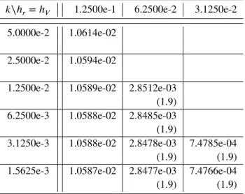
by two. In Table 1 , we present the numerical errors for the yields at maturity𝑇 = 10over the mesh grid: more specifically,

we show the maximum error over the grid points (the maximum norm). We observe that there exist values of the step sizes which do not provide satisfactory approximations: as usual in the literature a relation between the step sizes is necessary. Note that in each column the errors do not change practically: we do not obtain an increase in the accuracy under time refinement. However, in each row the errors go to zero as the step in the state variables decrease. Therefore, the error mainly comes from the discretization of the state variables. In order to observe the order of convergence, it is usual to compare the errors in the same diagonal. In this table, we show the experimental order of convergence in brackets, and we observe that it is of the second order.

𝑘∖ℎ_𝑟=ℎ_𝑉 1.2500e-1 6.2500e-2 3.1250e-2

5.0000e-2 1.0614e-02

2.5000e-2 1.0594e-02

1.2500e-2 1.0589e-02 2.8512e-03

(1.9)

6.2500e-3 1.0588e-02 2.8485e-03

(1.9)

3.1250e-3 1.0588e-02 2.8478e-03 7.4785e-04

(1.9) (1.9)

1.5625e-3 1.0587e-02 2.8477e-03 7.4766e-04

(1.9) (1.9)

TABLE 1 Errors for 10-year maturity yields obtained with the MHV method in test problem 1. In brackets, the experimental order of convergence comparing the diagonal entries.

Our next goal is to prove the efficiency of the MHV method. To this end, we measure this property by comparison of the accuracy offered with respect to the computational cost required. Again,𝑚_𝑟=𝑚_𝑣, that we denote as𝑀.

In Figure 1 , we present the results through a log-log efficiency chart where the vertical axis measures the errors in yields (in the maximum norm) and the horizontal axis corresponds to the cost (in CPU time). The stars joined by a solid line are the results of the method with𝑀= 4,8,12,16,20and𝑁= 100,200,300,400,500.

On the other hand, we compare the results with those obtained with another numerical technique very common in this kind of problems. In the finance literature, when a closed-form solution of a PIDE like (30) is unknown, it is usually expressed as the conditional expectation (5) by the Feynman-Kac Theorem. Then, zero-coupon bond prices are usually approximated by means

of MC method. This method approximates this expectation with a great number of paths of the state variables𝑟and𝑉. However,

this method involves a high computational cost and produces a low accuracy. For the test problem, we have carried out many

computations with different numbers of simulations, denoted by𝑆. In Figure 1 , the stars joined by the dashed line are the

results with the MC method for𝑆 = 2000,4000,16000,52000,60000. We observe that for a similar computational cost, the

MC method produces higher errors than the MHV method. In fact, in order to obtain 3 decimals of accuracy with this method we need a day of CPU time. However, with the MHV method this accuracy is obtained in less than a second of computation.

CPU

10-1 ₁₀0 ₁₀1 ₁₀2 ₁₀3 ₁₀4 ₁₀5

Error

10-4 10-3 10-2 10-1 100

MHV MC

FIGURE 1 Log-log efficiency chart for the 10-year yield approximations with the MHV and MC methods in test problem 1.

volatility

0 0.1 0.2 0.3 0.4 0.5

yield

-0.12 -0.1 -0.08 -0.06 -0.04 -0.02 0 0.02 0.04

0.06 r=5.5%

interest rate

0 0.05 0.1

yield

-0.05 -0.04 -0.03 -0.02 -0.01 0 0.01 0.02 0.03

v=0.175

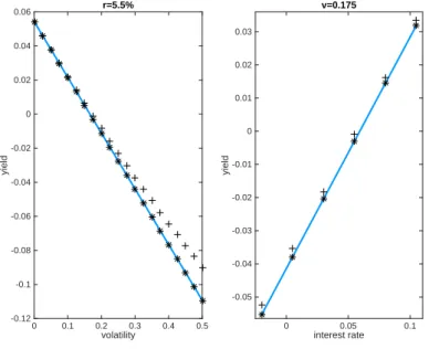
FIGURE 2 3-year yield profiles as function of the volatility when𝑟= 0.05(left), and the interest rate when𝑉 = 0.175(right) with the HV and MHV methods in test problem 1.

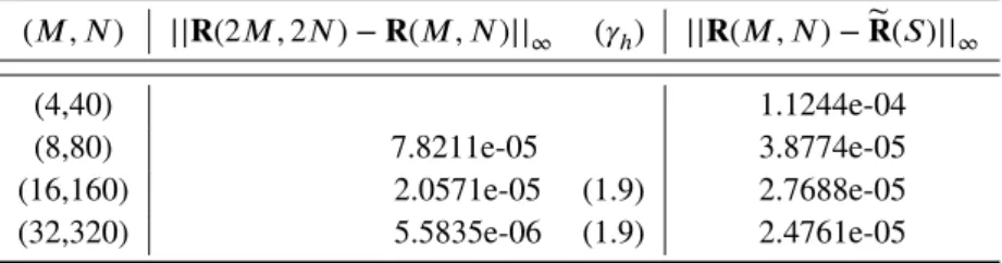
(𝑀 , 𝑁) ||𝐑(2𝑀 ,2𝑁) −𝐑(𝑀 , 𝑁)||∞ (𝛾ℎ) ||𝐑(𝑀 , 𝑁) −𝐑̃(𝑆)||∞

(4,40) 1.1244e-04

(8,80) 7.8211e-05 3.8774e-05

(16,160) 2.0571e-05 (1.9) 2.7688e-05

(32,320) 5.5835e-06 (1.9) 2.4761e-05

TABLE 2 Numerical results for the 10-year yields in test problem 2. Second column: comparison of consecutive approxima-tions obtained with the MHV method (experimental order of convergence in brackets). Third column: comparison of the MHV

approximations with the MC approximations (𝑆= 80000).

MHV method are the closest to the exact yields, they are practically the same. On the one hand, from the left picture the higher the volatility is, the higher the difference. But, from the right picture, the differences between the exact yields and those obtained with the usual boundary conditions increase slightly when the interest rates decrease. We have observed in our computations that, for greater values of the maturity the different behaviour is more remarkable.

Test problem 2: We study the interest rate model proposed by Cotton et al. 9_{. In this case, we have two state variables, the}

interest rate and another variable which provides the volatility of the interest rates. However, following (3), we add a jump term in the interest rate stochastic process. Then, the stochastic processes in this model are

𝑑𝑟= (𝑘₁(𝜇−𝑟) −𝜉𝑔(𝑠))𝑑𝑡+𝑔(𝑠)𝑑𝑊_𝑟+𝑑 ⎛ ⎜ ⎜ ⎝

𝑁(𝜆₎

∑

𝑖=1 𝑋_𝑖

⎞ ⎟ ⎟ ⎠ ,

𝑑𝑠=𝑘₂(𝛼−𝑠)𝑑𝑡+𝜂√𝑌 𝑑𝑊_𝑠.

In this case, we do not know a closed-form solution in order to compare the numerical approximations obtained by means of the

MHV method. For the numerical experiments, we consider the parameter values estimated in Cotton et al. 9_{, and we assume}

that the volatility of the interest rate is the positive function𝑔(𝑠) =e𝑠_{. Then, for pricing the corresponding zero-coupon bonds,} we have to solve the PIDE:

𝑝_𝜏= (𝑘₁(𝜇−𝑟) −𝜉e𝑠)𝑝_𝑟+𝑘₂(𝛼−𝑠)𝑝_𝑠+ 1 2e

2𝑠_𝑝 𝑟𝑟+

1 2𝜂

2_𝑠𝑝

𝑠𝑠+𝜌𝜂𝑠𝑝𝑟𝑠− (𝑟+𝜆)𝑝+𝜆 ∞

∫

−∞

𝑝(𝜏, 𝑟+𝑦, 𝑠)𝑓(𝑦)𝑑𝑦,

with the initial conditions (10).

We apply the proposed MHV method: we take the same truncated domain used in the previous test problem. We calculate the zero-coupon bond prices with a maturity equal to 10 years. In order to analyze the convergence of the approximations, taking into account that the solution is unknown, we compute the experimental order of convergence by means of the comparison

between two consecutive prices obtained by the refinement of the step sizes. Denoting by𝐑(2𝑀 ,2𝑁)the approximation at the

meshgrid of the yield obtained by the MHV method with𝑚_𝑟 =𝑚_𝑉 =𝑀, for the state variables, and𝑁, for the time variable,

we compute the experimental order of convergence in the standard way

𝛾_ℎ= log₂||𝑅(4𝑀 ,4𝑁) −𝑅(2𝑀 ,2𝑁)||∞

||𝑅(2𝑀 ,2𝑁) −𝑅(𝑀 , 𝑁)||_∞ . (31)

Second column of Table 2 shows the results, which are compatible with the expected order of convergence observed in the previous test problem. Finally, we compare the approximations provided by the MHV method with those computed with the

MC method, denoted bỹ𝐑(𝑆), where𝑆is the amount of simulations. Last column of Table 2 offers this comparison when

𝑆 = 80000, a sufficiently large number to assure that the approximation is hard to improve with the MC method. We observe the convergence of the MHV approximations to the same values obtained with the MC method.

5

CONCLUSIONS

In the finance literature, interest rate models are usually considered to be affine because a closed-form solution is always known. If the functions of the stochastic processes are assumed to be more realistic, an exact solution of the model is, in general, unknown. In such cases, numerical methods are the most important way to approximate the solution. On the one hand, the MC method is one of the most common techniques in the zero-coupon bond pricing. Although, it is very expensive from a computational point of view and not very accurate. On the other hand, other kind of methods, such as finite difference methods, require a bounded region for the state variables. However, this kind of problems typically involves a pure initial value problem.

When the interest rate is the single state variable, different numerical methods have been proposed for solving the pricing equation, jointly with well-stablished boundary conditions. Nevertheless, this is not the situation when there are two or more state variables: the usual conditions for the one-factor models expand the error from the boundary to all the integration interval. In this paper, we focus on approximating zero-coupon bond prices in a two-factor jump-diffusion model, where the state variables are the interest rates and the volatility. The problem consists of a partial integro-differential equation with a final condition. Then, for its numerical approximation, we introduce artificial boundaries in the domain that must be discretized. Here, we propose new boundary conditions based on the discount function properties of the bond prices. We discretize these boundary conditions and show how to incorporate them in an ADI method in order to approximate the solution.

An extensive numerical simulation in two different interest rate models shows that this new numerical procedure is a very valuable tool in the approximation of this kind of financial derivatives: it provides approximations of second order, is more efficient than the MC method and fits the profile of the solutions better than other artificial boundary conditions. Besides, this technique can be adapted easily to other numerical methods.

ACKNOWLEDGMENTS

This work has been supported in part by the project MTM2017-85476-C2-P of the Spanish Ministerio de Economía y Com-petitividad. Also by the projects VA041P17, VA138G18 and VA148G18 (Consejería de Educación de la Junta de Castilla y León).

References

1. Andersen T.G., Benzoni L., Lund J. Stochastic volatility, mean drift, and jumps in the short-term interest rate. Working Paper, Northwesterm University, University of Minnesota and Nykredit Bank, 2004.

2. Applebaum D.Lévy Processes and Stochastic Calculus.Cambridge, Cambridge University Press, 2009.

3. Bandi F.M., Nguyen T.H. On the functional estimation of jump-diffusion models.J. Econometrics2003; 116: 293-328.

4. Bremaud P.Point Processes and Queues. Martingale Dynamics. New York, Springer-Verlag New York, 1981.

5. Chernogorova T.P., Stehlikova B. A comparison of asymptotic analytical formulae with finite-difference approximation for

pricing zero coupon bond.Numer. Algor.2012; 59: 571-588.

6. Cont R., Tankov P.Financial Modeling with Jump Processes.Boca Raton, Florida, Chapman and Hall/CRC, 2004.

7. Cont R., Voltchkova E. A finite difference scheme for option pricing in jump diffusion and exponential Levy models.SIAM

J. Numer. Anal.2005; 43: 1596-1626.

8. Coonjobeharry R.K., Tangman D.Y., Bhuruth M. A novel partial integrodifferential equation-based framework for pricing

interest rate derivatives under jump-extended short-rate models.J. Comput. Finan.2015; 18: 129-161.

9. Cotton P., Fouque J.P., Papanicolaou G., Sircar R. Stochastic volatility corrections for interest rate derivatives.Math. Finan.

2004; 14: 173-200.

11. Das S.R., Foresi S. Exact solutions for bond and option prices with systematic jump risk.Rev. Deriv. Res.1996; 1: 7-24.

12. Duffy D.J.Finite Difference Methods in Financial Engineering: A Partial Differential Equation Approach.New York, John

Wiley & Sons, 2006.

13. Ekstrom E., Tysk J. Boundary conditions for the single-factor term structure equation.Ann. Appl. Probab.2011; 21:

332-350.

14. Fakharany M., Company R., Jodar L. Positive finite difference schemes for partial integro-differential option pricing model.

App. Math. Comp.2014; 249: 320-332.

15. Gómez-Valle L., Martínez-Rodríguez J. Estimation of risk-neutral processes in single-factor jump-diffusion interest rate

models.J. Comput. Appl. Math.2016; 291: 48–57.

16. Gómez-Valle L., Martínez-Rodríguez J. The risk-neutral stochastic volatility in interest rate models with jump-diffusion

processes.J. Comput. Appl. Math.2019; 347: 49–61.

17. Hong Y., Li H. Nonparametric specification testing for continuous-time models with applications to term structure of interest

rates.Rev. Financ. Stud.2005; 18: 37-84.

18. Hundsdorfer W. Accuracy and stability of splitting with stabilizing corrections.Appl. Numer. Math.2002; 42: 213-233.

19. in’t Hout K., Welfert B.D. Unconditional stability of second-order ADI schemes applied to multi-dimensional diffusion

equations with derivative terms.App. Num. Math.2009; 59: 677-692.

20. in’t Hout K., Toivanen J. ADI schemes for valuing European options under the Bates model.Appl. Numer. Math.2018; 130:

143-156.

21. in’t Hout K.,Numerical Partial Differential Equations in Finance Explained.London, Financial Engineering Explained,

Palgrave Macmillan, 2017.

22. Johannes M. The statistical and economic role of jumps in continuous-time interest rate models.J. Finan.2004; 59: 227-259.

23. Lin B.H. , Yeh S. K. Jump diffusion interest rate process: An empirical examination.J. Bus. Finan. Account.1999; 26:

967-995.

24. Oksendal B., Sulem A.Applied Stochastic Control of Jump Diffusions.Heidelberg, Springer Verlag, 2007.

25. Protter C.Stochastic Integration and Differential Equations.New York, Springer Verlag, 2004.

26. Shreve S.E.Stochastic Calculus for Finance II. Continuous-Time models. New York, Springer; 2008.