A novel fiber optic based surveillance system for prevention of pipeline integrity threats

Texto completo

(1)BIBLIOTECA. Document downloaded from the institutional repository of the University of Alcala: http://dspace.uah.es/dspace/. This is a postprint version of the following published document:. Tejedor, J., Macias-Guarasa, J., Martins, H.F., Piote, D., Pastor-Graells, J., Martin-Lopez, S., Corredera, P., Gonzalez-Herraez, M., 2017, "A novel fiber optic based surveillance system for prevention of pipeline integrity threats", Sensors (Switzerland), 17 (2), art. no. 355. Available at http://dx.doi.org/10.3390/s17020355. © 2017 The Authors (Article begins on next page). This work is licensed under a Creative Commons Attribution-NonCommercial-NoDerivatives 4.0 International License..

(2) Article. A Novel Fiber Optic Based Surveillance System for Prevention of Pipeline Integrity Threats Javier Tejedor1,† , Javier Macias-Guarasa2,∗ , Hugo F. Martins1 , Daniel Piote1 , Juan Pastor-Graells2 , Sonia Martin-Lopez2 , Pedro Corredera3 and Miguel Gonzalez-Herraez2 1 2 3. * †. FOCUS S.L., Spain; {javier.tejedor,hugo.martins,daniel.piote}@focustech.eu Department of Electronics, University of Alcalá, Spain; {macias,juan.pastor,sonia.martin,miguelg}@depeca.uah.es Instituto de Óptica, CSIC, Spain; p.corredera@csic.es Correspondence: macias@depeca.uah.es; Tel.: +34-91-885-6918 Current address: University CEU San Pablo, Spain; javier.tejedornoguerales@ceu.es. Academic Editor: name Version January 12, 2017 submitted to Sensors; Typeset by LATEX using class file mdpi.cls 1 2 3 4 5 6 7 8 9 10 11 12 13 14 15. 16 17. 18. 19 20 21 22 23 24 25 26. Abstract: This paper presents a novel surveillance system aimed at the detection and classification of threats in the vicinity of a long gas pipeline. The sensing system is based on phase-sensitive optical time domain reflectometry (φ-OTDR) technology for signal acquisition and pattern recognition strategies for threat identification. The proposal incorporates contextual information at feature level and applies a system combination strategy for pattern classification. The contextual information at feature level is based on the tandem approach (using feature representations produced by discriminatively trained multi-layer perceptrons) by employing feature vectors that spread different temporal contexts. The system combination strategy is based on a posterior combination of likelihoods computed from different pattern classification processes. The system operates in two different modes: (1) machine+activity identification, which recognizes the activity being carried out by a certain machine, and (2) threat detection, aimed at detecting threats no matter what the real activity being conducted is. In comparison with a previous system based on the same rigorous experimental setup, the results show that the system combination from the contextual feature information improves the results for each individual class in both operational modes, as well as the overall classification accuracy, with statistically significant improvements. Keywords: Distributed Acoustic Sensing; Fiber optic systems; φ-OTDR; Pipeline integrity threat monitoring; Feature-level contextual information; System combination. 1. Introduction Fiber optic distributed acoustic sensing (DAS) with phase-sensitive optical time-domain reflectometer (φ-OTDR) technology has been shown good performance for long perimeter monitorization aiming at detecting intruders on the ground [1–5], or vibration in general [6–14]. Current pipeline integrity prevention systems combine DAS technology and pattern recognition systems (PRS) for continuous monitoring of potential threats to the pipeline integrity [15–22]. In a previous work [22], we presented the first published report on a pipeline integrity threat detection and identification system that employs DAS+PRS technology, was evaluated on realistic field data, and whose results are based on a rigorous experimental setup and an objective evaluation. Submitted to Sensors, pages 1 – 19. www.mdpi.com/journal/sensors.

(3) Version January 12, 2017 submitted to Sensors. 27 28 29 30 31 32 33 34 35 36 37 38 39 40 41 42 43 44 45 46 47 48 49 50 51 52 53 54 55 56 57 58 59 60 61 62 63 64 65 66 67 68 69 70. 2 of 19. procedure with standard and clearly defined metrics1 . In [22] we did a thorough revision of all the previous published works in this area, showing their main limitations related to the pattern classification design: Classification results were not presented, there was a lack of rigorous and realistic experimental conditions (database building, signal acquisition in limited distances), or were aimed at a small number of classes (see [22] for more details). More recently, new works on this topic have been published: In [19], there is again a lack of realistic experimental conditions since all the signals corresponding to the same event are recorded in the same fiber position (hence biasing the system to recognize the position instead of the real event), the sensed area covers up to 20 kilometers (which reduces its application in realistic fiber deployments), and only 5 classes are employed. In [21], the sensing area spreads 24 kilometers and the real experiments were conducted at a fixed distance of 13 kilometers away from the sensor (which we demonstrated in [22] that was a major issue when facing realistic environments), dealing with only 3 classes. In addition, the number of tested signals in both works is small, with no additional details regarding the actual recording durations. Therefore, we can say that, again, these new systems do not fully address a realistic experimental setup that can assess the suitability of their proposals for realistic real time monitoring of long pipelines. The database used for the experiments in our previous work [22], which is composed of more than 1700 acoustic signals (about 10 hours of recordings), addresses all these issues: Different events were recorded and tested in different positions (covering different soil conditions) and different days (covering different environmental conditions) along a 40-kilometer pipeline. This, along with the adoption of a rigorous experimental procedure, allow us to state that the results are realistic enough to consider that similar performance can be obtained in field conditions. In what respect to the pattern recognition systems, one of the successful strategies used to improve their performance rates is adding contextual information [23]. For example, speech recognition systems obtain significant performance gains by incorporating context-dependent acoustic model information [24,25], or augmented features extracted from consecutive feature vectors (so-called first and second-order derivatives [26]). Image recognition systems also obtain significant improvements by incorporating contextual information within the final classification rule from multiple objects that appear in the image [27]. In the field of fiber optic sensing, contextual information has also been employed for temperature measurement [28,29]. Our previous work [22] addressed the contextual information in a limited extent, since the Short-Time Fast Fourier Transform (ST-FFT) employed in the feature extraction spreads only 1 second2 . Wavelets have also been employed previously to detect vibrations in distributed acoustic sensing systems, hence addressing contextual information to some extent as well [30]. Both approaches show a strategy based on adding sample-level contextual information, which means that the original signal is processed taking into account each sample context. However, the contextual information is usually applied within pattern classification systems at feature level [31– 34], once the high dimensionality present in the input signal is reduced to a more discriminative set of features, which is more relevant for classification. Another successful strategy to improve the performance of pattern recognition systems relies on system combination. This is based on the fact that complementary errors are provided by different pattern classification processes. Combination based on sum, product, average, or maximum rules [35–37], majority voting [35,37], or more advanced techniques such as logistic regression [38], Dempster-Shafer theory of evidence [37], and neural networks [36,37,39] have been applied to pattern. 1 2. The original system was developed under a GERG (The European Gas Research Group) supported project titled PIT-STOP (Early Detection of Pipeline Integrity Threats using a SmarT Fiber-OPtic Surveillance System). This was the optimal window size, after an intensive experimentation with shorter and longer window sizes for the ST-FFT, all of them leading to lower system performance..

(4) Version January 12, 2017 submitted to Sensors. 3 of 19. 72. recognition systems in different fields such as image recognition, speaker verification, handwritten recognition, and speech recognition, showing significant performance gains.. 73. 1.1. Motivation and Organization of the Paper. 71. 74 75 76 77 78. 79 80 81 82 83 84. 85 86 87 88 89 90 91 92. The pipeline integrity threat detection and identification system presented in previous works [15–22,40,41] did not make use of feature-level contextual information, nor exploited the possibility of combining results from different pattern recognition systems. Given the potential of both strategies, we propose to apply them on DAS+PRS technology for pipeline integrity threat detection and identification from two different perspectives: • Incorporating feature-level contextual information in an intelligent way, adapting the so-called tandem approach widely used in speech recognition [42] to enhance the feature vector of the baseline system. • Combining the outputs of different pattern classification processes, each of them using a combination of frequency-based and tandem features, exploiting different temporal ranges of contextual information. In this paper, we present (to the best of our knowledge) the first published report that incorporates contextual information at feature level and system combination in a DAS+PRS-based pipeline integrity threat detection and identification system, and is rigorously evaluated on realistic field data, showing significant and consistent improvements over our previous work [22]. The rest of the paper is organized as follows: The baseline system is briefly reviewed in Section 2, and Section 3 describes the novel pipeline integrity threat detection system. The experimental procedure is presented in Section 4 and the experimental results are discussed in Section 5. Finally, the conclusions are drawn in Section 6 along with some lines for future work.. Figure 1. Baseline version of the system architecture [22].. 93. 2. Baseline System. 94. 2.1. Sensing System. 95 96 97 98 99 100. The DAS system we used is a commercially available φ-OTDR-based sensor (named FINDAS) manufactured and distributed by FOCUS S.L. [43]. For interested readers, a full theoretical revision of the sensing principle, and a detailed description of the experimental setup used in the FINDAS sensor can be found in [44], but we provide here a short summary of the sensing strategy used. The φ-OTDR makes use of Rayleigh scattering — an elastic scattering (with no frequency shift) of light which originates from density fluctuations.

(5) Version January 12, 2017 submitted to Sensors. 4 of 19. 112. in the medium — to measure changes in the state of a fiber. In the FINDAS sensor employed, highly coherent optical pulses with a central wavelength near 1550 nm are injected into the optical fiber. The back-reflected signal from the fiber is then recorded, so that the interference pattern resultant from Rayleigh backscattering (φ-OTDR signal) is monitored at the same fiber input. By mapping the flight time of the light in the fiber, the φ-OTDR signal received at a certain time is associated with a fiber position. If vibrations occur at a certain position of the fiber, the relative positions of the Rayleigh scattering centers will be altered, and the φ-OTDR signal will be locally changed, thus allowing for distributed acoustic sensing [44]. The FINDAS has an (optical) spatial resolution of 5 meters (readout resolution of 1 meter) and a typical sensing range of up to 45 kilometers, using standard Single-Mode Fiber (SMF). A sampling frequency of f s = 1085 Hz was used for signal acquisition. A detailed description of the FINDAS technology can be found in [44].. 113. 2.2. Pattern Recognition System. 101 102 103 104 105 106 107 108 109 110 111. 114 115. 116 117 118 119. 120. 121 122 123 124 125 126. The baseline PRS was based on Gaussian Mixture Models (GMMs), and conducted classification in two different modes: 1. The machine+activity identification mode identifies the machine and the activity that the machine is conducting along the pipeline. 2. The threat detection mode directly identifies if the activity is an actual threat for the pipeline or not. The whole system integrated three main stages, as shown in Fig. 1: • Feature extraction, which reduces the high-dimensionality of the signals acquired with the DAS system to a more informative and discriminative set of features. • Feature vector normalization, which compensates for variabilities in the signal acquisition process and the sensed locations. • Pattern classification, which classifies the acoustic signal into a set of predefined NC classes (using a set of signal models, GMMs, previously trained from a labeled signal database).. 139. This system obtained promising results taking into account the ambitious experimental setup (i.e., recordings in a real industrial deployment). However, the absolute performance rate in machine+activity classification (45.15%, far better than the 12.5% chance rate for NC = 8 classes) is not still high enough for a practical system in field operations. Even though the threat/non-threat classification rates were much better (80% of threat detection and 40% of false alarms), strategies to improve both rates are necessary. The initial performance target that the GERG partners fixed to consider the system deployment in field was over 80% for the threat detection rate, and below 50% for the false alarm rate, so that these targets are actually achieved by the current proposal. In what respect to the performance target for the machine+activity identification rates, the GERG partners did not impose any specific requirements, as the crucial aspect for real world deployment is accurate threat-detection. Considering the difficulty of the task (with 8 different classes), identification rates in the range of 70% − 80% are reasonable to start with.. 140. 3. Novel Pipeline Integrity Threat Detection System. 127 128 129 130 131 132 133 134 135 136 137 138. 141 142 143 144 145 146. The proposal of the novel pipeline integrity threat detection system is presented in Fig. 2. First, the input acoustic signal is sent to a feature extraction module, where the energy corresponding to P frequency bands is calculated for the considered bandwidth f ∈ [ f 0 , f BW ], with f 0 and f BW being f the initial and final frequencies respectively, and f BW ≤ 2s . This builds NP -dimensional feature vectors (NP = 100). The feature normalization employed in this work is the sensitivity-based normalization described in Section III.B.2 of [22], where each coefficient of those feature vectors is.

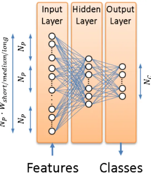
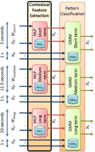
(6) Version January 12, 2017 submitted to Sensors. 5 of 19. Figure 2. Novel pipeline integrity threat detection system architecture. Modules in bold typeface are the new ones with respect to [22].. 158. normalized by the energy above the considered bandwidth. This was necessary due to the strong differences in the signals acquired in different sensing positions, which relate to the different soil conditions, the mechanical coupling of the fiber to the pipe enclosure, the machinery distance, the non-linear transduction function of a φ-OTDR-based sensor, the exponential decay of the amplitude of the measured signals along the fiber, etc. (see [22] for more details). The pattern classification module employs a GMM-based approach to classify each feature vector into the most likely class (machine+activity pair in the machine+activity identification mode that deals with NC = 8 classes, and threat/non-threat in the threat detection mode that deals with NC = 2 classes). This employs the a posteriori maximum probability criterion to assign the given feature vector the class with the highest probability given by the corresponding GMM. The additional blocks, the contextual feature extraction (that also needs a new previous training stage) and the decision combination are new with respect to our previous work [22], and are explained in more detail next.. 159. 3.1. Contextual Feature Extraction. 147 148 149 150 151 152 153 154 155 156 157. 160 161 162 163 164 165 166 167 168 169 170 171 172 173 174 175 176 177 178 179. The contextual feature extraction is based on the tandem approach used to compute the so-called tandem features in speech recognition tasks [45–47]. This module takes the normalized frequency-based feature vectors as input and produces tandem feature vectors as output. A multi-layer perceptron (MLP) is employed to integrate the feature-level contextual information. This MLP has three layers, as shown in Fig. 3: An input layer that consists of NP · Wsize feature vector values, where Wsize is the number of feature vectors used as contextual information (for an acoustic frame being analyzed at time t, the MLP will use the Wsize /2 feature vectors before t and the Wsize /2 feature vectors after t, along with the feature vector generated for time t), a hidden layer, whose number of units is selected based on preliminary experiments, and an output layer, with the number of units equals to the number of classes involved in the system modes (8 in the machine+activity identification mode and 2 in the threat detection mode). Specifically, three MLPs will be used to model the behavior of short, medium, and long temporal contexts, using Wshort , Wmedium , and Wlong feature temporal window sizes, respectively. The objective is effectively dealing with different signal behaviors that cope with short, medium, and long temporal contexts, so that a wider range of activities can be better learned by the system. In our implementation, the time lengths of each temporal context are 5 seconds, 12.5 seconds, and 20 seconds, corresponding to the short, medium, and long temporal contexts, respectively. These lengths were chosen based on the length of a single behavior within different activities. For example, for stable activities such as moving, long temporal windows are more suitable to model a single behavior. However, for more difficult activities (hitting or scrapping that include several behaviors), shorter.

(7) Version January 12, 2017 submitted to Sensors. 6 of 19. Figure 3. Architecture of the 3-layer MLP employed in the contextual feature extraction module.. 191. temporal windows are preferable so that the temporal windows used for modeling better cope with generating a robust model for a single behavior. Fig. 4 shows the detailed architecture of the contextual feature extraction module and its connection to the GMM-based pattern classification modules. The MLP models required for each temporal context (referred to as MLPS , MLP M , and MLP L in Fig. 4) are trained by the MLP training module in Fig. 2. The standard back-propagation algorithm [48] is employed to learn the MLP weights (i.e., connections between all the units of the input and hidden layers and connections between all the units of the hidden and output layers, as shown in Fig. 3). Therefore, three different sets of weights are learn (one for each temporal context), which are used next to obtain the posterior probability vectors. The contextual feature extraction involves two different stages, which are applied to each of the different temporal contexts:. 192. 3.1.1. Posterior probability vector computation. 180 181 182 183 184 185 186 187 188 189 190. 198. For each set of normalized feature vectors, and using the weights computed during MLP training, the MLP is employed to calculate a posterior probability for each class to be identified. This process is similar to use the MLP for classification. However, instead of assigning a raw class label to each normalized feature vector, the MLP outputs (consisting of one posterior probability per class, as shown in Fig. 3) are used as new features. This builds a set of NC -dimensional posterior probability vectors per MLP (i.e., per temporal context), as shown in Fig. 4.. 199. 3.1.2. Tandem feature vector building. 193 194 195 196 197. 200 201 202 203 204 205 206 207 208. This stage concatenates the original NP -dimensional feature vectors (those generated by the feature normalization module), and the NC -dimensional posterior probability vectors computed by the MLPs. Therefore, ( NP + NC )-dimensional tandem feature vectors are built (in our implementation, NP + NC = 108 for the machine+activity identification mode, and NP + NC = 102 for the threat detection mode). These are fed into three different pattern classification processes (one for each temporal context), which generate a likelihood value for each of the NC classes, as shown in Fig. 4. It must be noted that the GMM training is also carried out from these tandem feature vectors. For MLP training, posterior probability vector computation, and tandem feature vector building, the ICSI QuickNet toolkit [49] has been employed..

(8) Version January 12, 2017 submitted to Sensors. 7 of 19. Figure 4. Detailed architecture of the contextual feature extraction module and its connection to the GMM-based pattern classification modules..

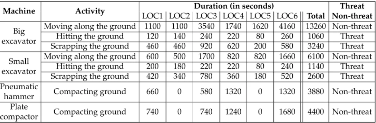
(9) Version January 12, 2017 submitted to Sensors. 209. 8 of 19. 3.2. Decision Combination. 214. Given the three pattern classification processes conducted on the tandem feature vectors that cover different temporal contexts, and in order to exploit their complementarity when dealing with different activities, a way to combine their outputs is necessary. In this work, we have evaluated three methods to carry out a likelihood-based combination: Sum, Product, and Maximum, which are presented next:. 215. 3.2.1. Sum method. 210 211 212 213. 216. For any frame (i.e., feature vector), the likelihood assigned to each class ci is given by: N. l ( ci ) =. ∑ l j ( c i ),. (1). j =1. 220. where N is the number of classification processes, and l j (ci ) is the likelihood assigned to class ci in the classification process j. This sum method is typically better adapted for cases in which each classifier performs different [50].. 221. 3.2.2. Product method. 217 218 219. 222. For any frame, the likelihood assigned to each class ci is given by: N. l ( ci ) =. ∏ l j ( c i ).. (2). j =1. 224. This product method is typically better adapted for systems where the feature sets are independent [51].. 225. 3.2.3. Maximum method. 223. 226. For any frame, the likelihood assigned to each class ci is given by: N. l (ci ) = max l j (ci ). j =1. 227 228 229 230. (3). This maximum method is typically better adapted for systems where the performance of each individual classifier is similar [50]. For all the combination methods, the class that is finally assigned to each frame as the recognized one is given by the maximum a posteriori criterion: ĉ = argmax {l (ci )}.. (4). i. 232. The combination approach can be applied to all the classification processes, or to a selection of them, so that a fruitful experimentation can be carried out.. 233. 4. Experimental Procedure. 231. 235. Our experimental setup is basically the same than that described in Section IV of [22]. We provide here the fundamental details, referring the reader to the original paper for further details.. 236. 4.1. Database Description. 234. 237 238. For comparison purposes, we employed the same database as in our previous work [22], whose content is summarized in Table 1..

(10) Version January 12, 2017 submitted to Sensors. 239 240 241 242 243 244 245 246 247 248 249 250 251 252 253 254 255 256 257 258 259 260 261 262 263 264 265 266 267 268 269 270 271 272 273 274 275 276 277 278 279 280 281 282 283 284. 9 of 19. As described in [22], an active gas transmission pipeline operated by Fluxys Belgium S.A. was used for the database acquisition, thus operating in a real scenario. The pipeline is made from steel, has a diameter of 1 meter, and is 1 inch thick. Activities nearby the pipeline were sensed by monitoring an optical fiber cable installed about 0.5 meters from the pipeline and parallel to it (the fiber cable installation was done at the same time of the pipeline construction). The pipeline and the associated optical fiber are buried, and the pipeline is pressurized at 100 bars (being an active one, operating in normal conditions). The fiber depth varies between 0.3 and 2 meters, and since it does not follow a tight parallel path along the pipeline, and in some points there are fiber rolls for maintenance purposes, a calibration procedure between fiber distance and geographical location was carried out for precise location labeling. The selected activities cover realistic situations (involving possible threats and harmless ones) that could typically occur nearby pipeline locations. All of them were carefully selected by the GERG partners within the PIT-STOP project, and represented those activities that could provide the best assessment of the system capabilities for real world deployment. In particular, the staff at Fluxys Belgium S.A. (the gas carrier company in this country) was responsible for the proposal of the activities to be carried out for evaluation. On the one hand, the dangerous activities (hitting and scrapping by small and big excavators), allowed the system to be tested when a real threat for the pipeline occurs (as it is the usual situation before a critical pipeline “touch” happens). On the other hand, the non-threat activities were chosen based on their high-occurrence rate near pipelines (movements of different machinery, and non-dangerous activities performed by pneumatic hammer and plate compactor machines). The FINDAS sensor is connected at one end of the fiber that runs in parallel to the inspected pipeline. The different locations (LOC1, LOC2, LOC3, LOC4, LOC5, and LOC6) cover different pipeline “reference positions” selected at high distances from the sensing equipment (being at 22.24, 22.49, 23.75, 27.43, 27.53, and 34.27 kilometers far from the FINDAS box respectively) to evaluate the system in conditions close to the actual sensing limits and to ensure feature variabilities in terms of soil characteristics and weather conditions (see [22] for more details). The machines used for the recordings of the different machine+activity pairs started their activity at the center of the so-called “Machine operation area” (see Fig. 5 for a visual reference). This area was located at distances between 0 meters (on top of the fiber), and up to 50 meters from the so-called “Reference position” right above the pipeline3 . The “hitting” and “scrapping” activities were recorded five times in different positions within the machine operation area (the first position was located in the center of the area, and the other four were located at ±25 meters and ±50 meters from this center, with direction depending on the available space around the operation area). The “movement” and “compacting” activities spread around ±25 meters from the center of the operation area. These two activities were recorded in two different ways: the first one comprises both movement and compacting actions when the machine is carrying out the activity parallel to the pipeline, being the second one with the activity carried out perpendicular to the pipeline. This allowed us to generate different acoustic patterns corresponding to both ways, hence obtaining a more varied database. From this “Reference position”, the signals were captured from the optical fiber in a ±200 meter interval (see Fig. 5), with 1 meter spacing, thus generating 400 acoustic traces for each recorded activity. This 400-meter interval was selected to ensure that we had a wide enough range of fiber responses to be used in the training and evaluation procedures. Although the distance of the acoustic source (the machine performing the given activity) to the optical fiber has an impact on the signal-to-noise ratio (SNR), the high sensitivity of the sensing system. 3. As described in [22] in the recording protocol for each location, the reference position was chosen manually as the closest to the center of the operation area with good sensitivity, by real time monitoring of the fiber response..

(11) Version January 12, 2017 submitted to Sensors. 10 of 19. Table 1. Experimental database. ‘Big excavator’ is a 5 ton Kubota KX161-3. ‘Small excavator’ is a 1.5 ton Kubota KX41-3V. From [22]. Duration (in seconds) LOC1 LOC2 LOC3 LOC4 LOC5 Moving along the ground 1100 1100 3540 1740 1620 Big Hitting the ground 120 140 240 220 80 excavator Scrapping the ground 460 460 920 620 200 Moving along the ground 600 500 1700 820 820 Small Hitting the ground 200 180 220 220 80 excavator Scrapping the ground 420 340 780 360 180 Pneumatic Compacting ground 660 0 580 1320 0 hammer Plate Compacting ground 740 0 740 1240 0 compactor Machine. Activity. Threat LOC6 Total Non-threat 4160 13260 Non-threat 260 1060 Threat 580 3240 Threat 1660 6100 Non-threat 240 1140 Threat 520 2600 Threat 1320. 3880. Non-threat. 1680. 4400. Non-threat. 287. within the limits of the selected “Machine operation area” for each location makes the SNR to be good enough to cover realistic and practical situations. Moreover, the trained signal models are also able to cope with this variability due to the acoustic source distance to the pipeline.. 288. 4.2. System Configuration. 285 286. 289 290 291 292 293 294 295 296 297 298. Regarding the feature extraction, the relevant parameters are as follows: The acoustic frame size was set to 1 second, the acoustic frame shift was set to 5 milliseconds, the number of FFT points was set to 8192, the number of frequency bands (i.e., the original feature vector size) was set to 100, and the initial and final frequencies corresponding to the analyzed bandwidth were set to 1 Hz and 100 Hz respectively. The highest energy meter selection in our previous work has been selected for signal representation, due to its better performance over the reference position (see Fig. 5) [22]. Therefore, each acoustic frame used either for training or evaluation (MLP in the contextual feature extraction and GMM in the pattern classification) corresponds to the highest energy meter between those acquired by FINDAS. Pipeline. ed rd e co sid re s s hi er t t et a m RP 0 20 rom f. LOC6. Reference position (RP) ed rd e co sid re s his er t et at m RP 0 20 rom f. Machinery operation area. Fiber Recorded ﬁber segment. Figure 5. Recording scenario: Real example at LOC6, taken from [22]. 299 300 301 302. For the contextual feature extraction, 100 units have been used in the hidden layer for MLP training and posterior probability vector computation for the machine+activity identification mode, and 3 units for the threat detection mode. These values were chosen based on their best performance in preliminary experiments..

(12) Version January 12, 2017 submitted to Sensors. 11 of 19. 317. For pattern classification, a single GMM component has been used to model each class in both modes. The use of the sensitivity-based normalization and the bandwidth limited to 100 Hz is explicitly designed to also help in dealing with the noise in the raw data. The normalization aids in equalizing noise effects compensating for variabilities in the signal acquisition process and the sensed location (as background noise can vary for different locations due to the proximity of road, factories, etc.), and the bandwidth limitation avoids considering noisy signals where no relevant information is to be found. Also, while variations in the fiber temperature could introduce noise in the measurements, these typically occur at much lower frequencies than the processed acoustic signals so that they do not constitute a relevant issue in our proposal. Nevertheless, even though the raw signals have a high level of noise (as shown in the sample signal spectrograms shown in Fig. 2 of [22]), each machine+activity pair exhibits, in general, a reasonably consistent spectral behavior, hence allowing for the use of pattern classification strategies that can efficiently extract this consistent behavior. A full experimental and theoretical description of the optical noise characteristic of the DAS technology using a similar setup, which defines the background noise of the raw data, can be found in [44].. 318. 4.3. Evaluation Strategy. 303 304 305 306 307 308 309 310 311 312 313 314 315 316. 337. The evaluation strategy was carefully and rigorously designed to maximize the statistical significance of the results and to provide a wide variety in the design of the training and evaluation subsets. With this objective, the robust and widely adopted leave-one-out cross-validation (CV) strategy [52] was selected to carry out the experiments. The criteria to split the full database in training and evaluation subsets match with the recorded data location criteria. Since data were recorded in 6 different locations, the CV strategy comprises 6 folds, where the data recorded in all the locations except one were used for training (including MLP training and posterior probability vector computation for the contextual feature extraction and GMM training for the pattern classification), and the evaluation was done on data of the unused location (thus ensuring full independence between the training and evaluation subsets). Classification is again conducted on a frame-by-frame basis. Using the data from the same locations for MLP training and posterior probability vector computation in the contextual feature extraction could lead to overfitting problems, since a subset of the data employed for MLP training is also used to compute the posterior probability values of the tandem feature vectors employed for training the pattern classification module. To evaluate this drawback, we ran a full set of experiments in which different locations for MLP training and posterior probability vector computation were employed, and similar results are obtained, which clearly indicates that no overfitting occurs.. 338. 4.4. Evaluation Metrics. 319 320 321 322 323 324 325 326 327 328 329 330 331 332 333 334 335 336. 339 340 341 342 343 344 345 346. As in our previous work [22], and for comparison purposes, the classification accuracy has been the main metric to evaluate the system performance both for the machine+activity identification and threat detection modes. In addition, we will also show the class classification accuracy for the machine+activity identification mode, and the threat detection rate and false alarm rate for the threat detection mode. Finally, to provide a full picture of the classification performance we will also show the confusion matrix (i.e., a table that shows the percentage of evaluation frames of a given class that are classified as any of the considered classes) for the machine+activity identification mode. Statistical validation of the results will be provided to assess the statistical significance of the results..

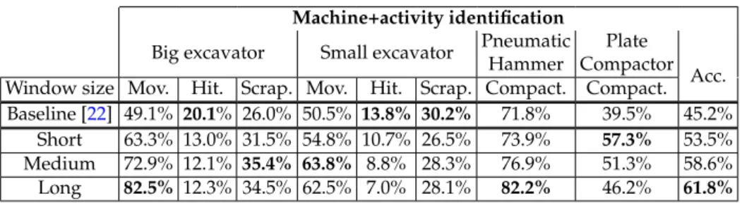
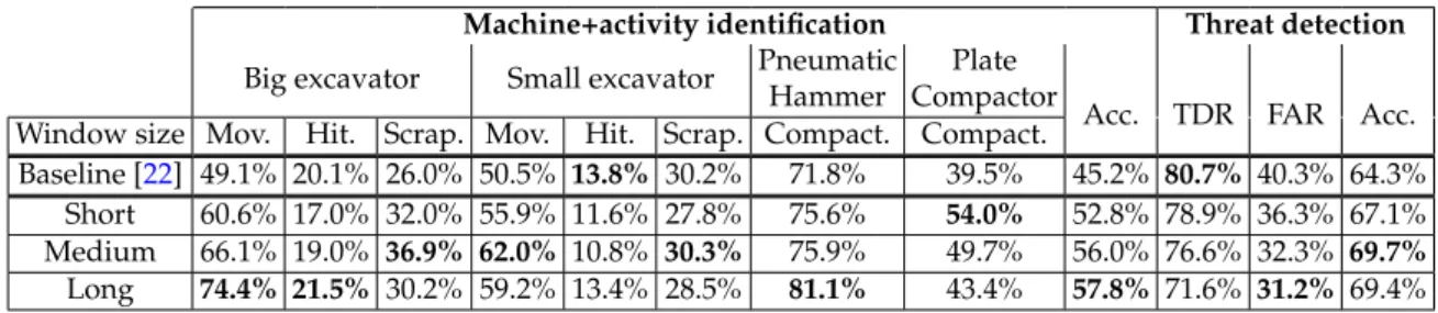
(13) Version January 12, 2017 submitted to Sensors. 12 of 19. Table 2. MLP classification accuracy for the machine+activity identification mode for every class with various window sizes with the best result for each class in bold font. ‘Acc.’ is the overall classification accuracy, with the best result in bold font. ‘Mov.’ stands for moving, ‘Hit.’ stands for hitting, ‘Scrap.’ stands for scrapping, and ‘Compact.’ stands for compacting. Machine+activity identification Pneumatic Plate Big excavator Small excavator Hammer Compactor Acc. Window size Mov. Hit. Scrap. Mov. Hit. Scrap. Compact. Compact. Baseline [22] 49.1% 20.1% 26.0% 50.5% 13.8% 30.2% 71.8% 39.5% 45.2% Short 63.3% 13.0% 31.5% 54.8% 10.7% 26.5% 73.9% 57.3% 53.5% Medium 72.9% 12.1% 35.4% 63.8% 8.8% 28.3% 76.9% 51.3% 58.6% Long 82.5% 12.3% 34.5% 62.5% 7.0% 28.1% 82.2% 46.2% 61.8%. 347. 5. Experimental Results. 348. 5.1. Preliminary Experiments. 373. A preliminary set of experiments was run to show the potential effectiveness of (1) using contextual information, and (2) combining different contextual information sources in the whole system. This set of experiments takes the 100-dimensional normalized feature vectors as input for the MLP and conducts classification. For MLP-based classification, we simply assign the class with the highest posterior probability as the recognized class with which we can evaluate the system performance. The different temporal contexts (short, medium, and long) are employed for MLP training and classification, and the obtained results are presented in Table 2. From Table 2, it is clearly seen that, even though the overall accuracy improves when increasing the temporal context, the optimal temporal context (short, medium, or long) is different for each machine+activity pair (best rates are shown in bold). For example, for the big excavator moving, the baseline performance is 49.1%, and this increases to 63.3%, 72.9%, and 82.5% when using progressively longer temporal contexts (short, medium, and long, respectively). On the other hand, for the small excavator hitting, increasing the temporal context leads to systematic performance degradation from the 13.8% obtained in the baseline to 10.7%, 8.8%, and 7.0% for progressively longer temporal contexts. These results indicate that different temporal contexts model the feature space in a different way, so that employing and combining different window sizes could bring further improvements to the whole system performance (thus motivating our combination approach). In addition, the MLP does not seem to be suitable to replace the GMM for classification. Despite the best overall performance obtained with the long-length window size, there are some classes whose performance is worse than that of the baseline (hitting and scrapping activities with the small excavator, and hitting activity with the big excavator, which include multiple behaviors and have the less amount of training data). Therefore, this motivates the use of the MLP to produce a tandem feature vector and to maintain the GMM-based pattern classification system.. 374. 5.2. Contextual Feature Extraction. 349 350 351 352 353 354 355 356 357 358 359 360 361 362 363 364 365 366 367 368 369 370 371 372. 375 376 377 378 379 380 381. We analyze the performance of the contextual feature extraction module from the tandem feature vectors that are built from different window sizes. To do so, a GMM-based pattern classification process is carried out for each of the proposed temporal contexts (short, medium, and long), as shown in Fig. 4, and results are presented in Table 3. At first sight, for the machine+activity identification mode, the average system performance compared with the baseline (column Acc. in Table 3) seems to improve to a great extent (57.8% − 45.2% = 12.6% absolute improvement). Paired t-tests [53] show that this improvement is statistically.

(14) Version January 12, 2017 submitted to Sensors. 13 of 19. Table 3. Contextual feature extraction module results. Class classification accuracy and overall classification accuracy for the machine+activity identification mode, and threat detection rate (TDR), false alarm rate (FAR), and overall classification accuracy for the threat detection mode, with the best results in bold font. ‘Acc.’, ‘Mov.’, ‘Hit.’, ‘Scrap.’, and ‘Compact.’ denote the same as in Table 2. Machine+activity identification Threat detection Pneumatic Plate Big excavator Small excavator Hammer Compactor Acc. TDR FAR Acc. Window size Mov. Hit. Scrap. Mov. Hit. Scrap. Compact. Compact. Baseline [22] 49.1% 20.1% 26.0% 50.5% 13.8% 30.2% 71.8% 39.5% 45.2% 80.7% 40.3% 64.3% Short 60.6% 17.0% 32.0% 55.9% 11.6% 27.8% 75.6% 54.0% 52.8% 78.9% 36.3% 67.1% Medium 66.1% 19.0% 36.9% 62.0% 10.8% 30.3% 75.9% 49.7% 56.0% 76.6% 32.3% 69.7% Long 74.4% 21.5% 30.2% 59.2% 13.4% 28.5% 81.1% 43.4% 57.8% 71.6% 31.2% 69.4%. 382 383 384 385 386 387 388 389 390 391 392 393 394 395 396 397 398 399 400 401 402 403 404 405 406 407 408 409 410 411 412 413 414 415 416. significant for any window size over the baseline (p < 10−32 ). However, looking at the individual class performance, this improvement is not that clear. There are classes for which very similar or even slightly worse performance is obtained with the tandem feature vectors (e.g., small excavator doing hitting (13.8% for the baseline system and 13.4% for the tandem system) and scrapping (30.2% for the baseline system and 30.3% for the tandem system)), and the best performance for each class largely depends on the window size. The large improvement obtained with the tandem feature vectors is for the classes for which more data are available. For example, the moving activity from the big excavator improves the 49.1% baseline performance to 74.4% for the tandem system, and from the small excavator the improvement goes from the 50.5% baseline performance to 62.0%. Also, large improvements are observed for the plate compactor (from 39.5% to 54.0%) and the pneumatic hammer (from 71.8% to 81.1%). The fact that more data are available for these classes is biasing the performance calculation, but we also have to consider the effect on the classes with lower performance. The high performance classes, which tend to have a more stable behavior, get much more benefit from the feature-level contextual information than classes that represent different acoustic behaviors (i.e., hitting and scrapping activities). The greater amount of training data of those classes also contributes to this, since a more robust GMM is trained. On the contrary, for classes with different acoustic behaviors during its execution (hitting and scrapping), integrating these multiple behaviors could lead to less robust GMMs, so that the final performance for these classes is similar or even worse than that of the baseline. For example, for the small excavator hitting, there is a performance degradation from the baseline 13.8% to 13.4%. The only exception for this observation is the improvement obtained for the big excavator doing scrapping (36.9% versus 26.0% of the baseline), which may be due to the greater amount of training data available, so that a more robust GMM is built. This suggests that using feature-level contextual information in isolation is not enough to obtain the best performance in the whole system for classes for which different acoustic behaviors are observed and the amount of data used to train the GMM is limited. For the threat detection mode, it can be seen that incorporating feature-level contextual information also provides an improvement in the overall classification accuracy over the baseline (69.7% − 64.3% = 5.4% absolute improvement). Paired t-tests show that this improvement is statistically significant for any window size (p < 10−24 ) over the baseline. However, by inspecting the threat detection rate and the false alarm rate, it can be seen that both figures decrease compared with those of the baseline, which makes more difficult derive a clear conclusion. From these results, we can state that decision combination is necessary to take advantage of the complementary classification errors obtained for each temporal context..

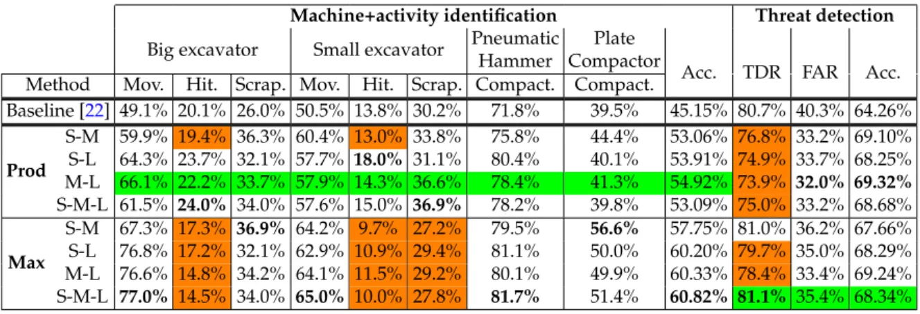
(15) Version January 12, 2017 submitted to Sensors. 14 of 19. Table 4. Decision combination results. Class classification accuracy and overall classification accuracy for the machine+activity identification mode, and threat detection rate (TDR), false alarm rate (FAR), and overall classification accuracy for the threat detection mode with the best results in bold font. For combination, ‘Prod’ is the Product method and ‘Max’ is the Maximum method. ‘S’ denotes short window size, ‘M’ denotes medium window size, and ‘L’ denotes long window size. ‘Acc.’, ‘Mov.’, ‘Hit.’, ‘Scrap.’, and ‘Compact.’ denote the same as in Table 2. Machine+activity identification Threat detection Pneumatic Plate Big excavator Small excavator Hammer Compactor Acc. TDR FAR Acc. Method Mov. Hit. Scrap. Mov. Hit. Scrap. Compact. Compact. Baseline [22] 49.1% 20.1% 26.0% 50.5% 13.8% 30.2% 71.8% 39.5% 45.15% 80.7% 40.3% 64.26% S-M 59.9% 19.4% 36.3% 60.4% 13.0% 33.8% 75.8% 44.4% 53.06% 76.8% 33.2% 69.10% S-L 64.3% 23.7% 32.1% 57.7% 18.0% 31.1% 80.4% 40.1% 53.91% 74.9% 33.7% 68.25% Prod M-L 66.1% 22.2% 33.7% 57.9% 14.3% 36.6% 78.4% 41.3% 54.92% 73.9% 32.0% 69.32% S-M-L 61.5% 24.0% 34.0% 57.6% 15.0% 36.9% 78.2% 39.8% 53.09% 75.0% 33.2% 68.68% S-M 67.3% 17.3% 36.9% 64.2% 9.7% 27.2% 79.5% 56.6% 57.75% 81.0% 36.2% 67.66% S-L 76.8% 17.2% 32.1% 62.9% 10.9% 29.4% 81.1% 50.0% 60.20% 79.7% 35.0% 68.29% Max M-L 76.6% 14.8% 34.2% 64.1% 11.5% 29.2% 80.1% 49.9% 60.33% 78.4% 33.4% 69.24% S-M-L 77.0% 14.5% 34.0% 65.0% 10.0% 27.8% 81.7% 51.4% 60.82% 81.1% 35.4% 68.34%. 417. 5.3. Decision Combination. 425. Decision combination employs different combinations of temporal contexts (in pairs, or all of them) to make the final decision for each frame. Results are shown in Table 4 for the machine+activity identification mode and the threat detection mode. To ease the analysis, the results for the Sum method are not shown as they are almost identical to those obtained with the Product method. Additionally, the cells with worse results than the baseline have an orange background, and the green background cells indicate the selected systems for the machine+activity identification and threat detection modes. As it can be seen, almost all the results obtained with the decision combination improve those of the baseline.. 426. 5.3.1. Machine+activity identification mode. 418 419 420 421 422 423 424. 427 428 429 430 431 432 433 434 435 436 437 438 439 440 441 442 443 444 445 446. For the machine+activity identification mode, the combination of any window size with any combination method outperforms the overall classification accuracy of the baseline in a great extent (52.91% − 45.15% = 7.76% minimum absolute improvement, which means a 17% relative improvement). Paired t-tests show that this improvement is statistically significant for all the cases (p < 10−30 ). For Sum and Product methods, consistent performance gains are obtained for all the classes in general. Sum method is expected to work well when each individual classifier performs quite different [50], as is our case (see Table 3). Product method is also expected to derive a robust combination when the feature sets are independent [51]. Different temporal contexts model the feature space in a different way so that the feature set for every class can be considered as independent. For hitting and scrapping activities, which possess multiple behaviors and have the less amount of training data, the performance obtained with the Maximum method is much worse than that of the baseline (for example, for the small excavator hitting, the 13.8% baseline gets as low as 9.7%). This can be due to two reasons: (1) The Maximum method does not integrate information of different classification processes (only the best likelihood is selected), which for multi-class classification problems is important, and (2) this method provides gains when the performance of the individual classifiers is close, which is not our case (see Table 3). The only exception is again for the big excavator doing scrapping, for which performance gains are obtained for each combination method (from the 26.0% baseline performance up to 36.3% with the Product Method and 36.9% with the Maximum.

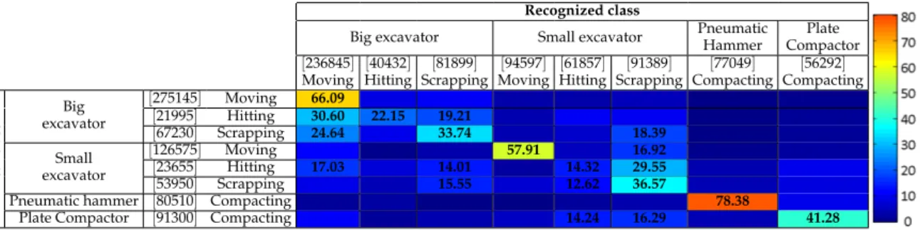
(16) Version January 12, 2017 submitted to Sensors. 15 of 19. Table 5. Confusion matrix of the Product combination method from medium and long window sizes for the machine+activity identification mode. Classification Accuracy is shown in each cell. The values between brackets represent the number of frames that are classified as the recognized class, or that belong to the real class. Recognized class Pneumatic Plate Hammer Compactor [236845] [40432] [81899] [94597] [61857] [91389] [77049] [56292] Moving Hitting Scrapping Moving Hitting Scrapping Compacting Compacting [275145] Moving 66.09 Big [21995] Hitting 30.60 22.15 19.21 excavator [67230] Scrapping 24.64 33.74 18.39 [126575] Moving 57.91 16.92 Small [23655] Hitting 17.03 14.01 14.32 29.55 excavator [53950] Scrapping 15.55 12.62 36.57 Pneumatic hammer [80510] Compacting 78.38 Plate Compactor [91300] Compacting 14.24 16.29 41.28. Real class. Big excavator. Small excavator. Table 6. Machine+activity identification mode rate comparison between the baseline and novel systems. Relative improvement is calculated as 100 · Big excavator Baseline Novel Relative improvement. 447 448 449 450 451 452 453 454 455 456 457 458 459 460 461 462 463 464 465 466 467 468 469 470. Moving 49.05% 66.09% 34.74%. Hitting 20.11% 22.15% 10.14%. Scrapping 26.03% 33.74% 29.62%. (novelaccuracy −baselineaccuracy ) . baselineaccuracy. Small excavator Moving 50.50% 57.9% 12.89%. Hitting 13.78% 14.32% 3.92%. Scrapping 30.22% 36.57% 21.01%. Pneumatic Hammer Compacting 71.84% 78.38% 9.10%. Plate Compactor Compacting 39.51% 41.28% 4.48%. Averages 45.15% 54.92% 21.30%. method). This may be again due to the availability of more training data, which results in a more robust GMM. Our selection proposal is the Product-based combination from medium and long temporal window sizes, since this presents the best overall accuracy with consistent improvements for each individual class. Table 5 shows the corresponding confusion matrix of this combination, where we have removed the values below chance (1/8 = 12.5%) to ease the visualization and analysis, and where we have used color information as a visual aid. In general, it is clearly seen that the diagonal contains the greatest figures for each class (with at least 9% absolute better accuracy compared to the second most recognized one, i.e., 33.74%-24.64%=9.10% in the big excavator doing scrapping), except for the hitting activity. For the big excavator, this is confused with the moving and scrapping activities. On the one hand, the big excavator doing hitting has the less amount of training data, which can cause that the classification process prefers the GMM for which more training data are available. On the other hand, scrapping also includes hitting when the shovel contacts the ground, which is also causing confusion in the small excavator. The classes with the lowest performances correspond to the hitting and scrapping activities, which are also confused between each other. On the one hand, these are the classes with the less amount of training data, which derives in a less robust GMM. In addition, hitting and scrapping activities present different acoustic behaviors (moving up the shovel, moving it down, hitting, scrapping, moving, etc.), which may degrade the GMM, since just a single GMM component is used for modeling.4 It is also important to note the significant improvements in the identification rates with respect to the baseline system, as shown in Table 6. The relative performance improvement between the baseline and novel systems range from 4.48% up to 37.74%, with an average value of 21.30%, which clearly validates the strategy used towards improving the overall performance.. 4. Increasing the number of GMM components does not provide any gain, probably due to the small amount of training data for these classes..

(17) Version January 12, 2017 submitted to Sensors. 471. 16 of 19. 5.3.2. Threat detection mode. 483. For the threat detection mode, the overall classification accuracy shows a similar trend. All the method combinations for any window size significantly outperform the baseline (p < 10−26 for a paired t-test). Combining all the temporal window sizes with the Maximum method outperforms the baseline both for the threat detection rate (from the 80.7% baseline performance up to 81.1%, which implies a relative improvement of 0.5%), and false alarm rate (from the 40.3% baseline performance down to 35.4%, which implies a relative improvement of 12%). These improvements are significant for the threat detection rate (p < 10−5 ) and for the false alarm rate (p < 10−28 ). By integrating all the window sizes in a small classification task (two classes: threat/non-threat) the feature space is modeled in such a different way that the pattern classification makes different and complementary errors, so that the final performance gets improved in the Maximum method, for which the classifier with the highest likelihood takes the final decision.. 484. 6. Conclusions and Future Work. 472 473 474 475 476 477 478 479 480 481 482. 485 486 487 488 489 490 491 492 493 494 495 496 497 498 499 500 501 502 503 504 505 506 507 508 509 510 511 512 513 514. This paper has presented a novel approach for a pipeline integrity threat detection system that employs a φ-OTDR fiber optic-based sensing system for data acquisition by adding feature-level contextual information and system combination in the pattern recognition stage. The proposal achieves consistent and significant improvements that were verified in a machine+activity identification task, where the machine and the activity carried out must be known, and in a threat detection task, where just the occurrence of a threat for the pipeline has to be known. Feature-level contextual information in isolation has been shown to perform well for machine+activity pairs that possess a stable behavior and for which enough training data are available. Adding the decision combination from different pattern recognition processes that run on different contextual information window sizes has been shown to outperform the overall classification accuracy and the class classification accuracy for both tasks. Although the results presented in this paper have improved those of the baseline in a great extent (about 21% relative in the machine+activity identification mode, and 12% relative in the false alarm rate with a slight improvement of 0.5% relative in the threat detection rate for the threat detection mode), there is still much work to do. For classes for which different behaviors exist and the amount of training data is low, the improvements obtained are not as high as for the rest of the classes. Therefore, future work should focus on these low-performance classes by, for example, developing new strategies that will also extend our system to make use of contextual information in the spatial domain (that is by using the acoustic traces from nearby sensed positions, which should experience similar disturbances simultaneously). Acknowledgments: Some authors were supported by funding from the European Research Council through Starting Grant UFINE (grant number #307441), Water JPI, the WaterWorks2014 Cofunded Call, the European Commission (Horizon 2020) through project H2020-MSCA-ITN-2016/722509 - FINESSE, the Spanish Ministry of Economy and Competivity, the Spanish “Plan Nacional de I+D+i” through projects TEC2013-45265-R, TEC2015-71127-C2-2-R, TIN2013-47630-C2-1-R and TIN2016-75982-C2-1-R, and the regional program SINFOTONCM: S2013/MIT-2790 funded by the “Comunidad de Madrid”. HFM acknowledges funding through the FP7 ITN ICONE program, grant number #608099 funded by the European Commission. JPG acknowledges funding from the Spanish Ministry of Economy and Competivity through an FPI contract. SML acknowledges funding from the Spanish Ministry of Science and Innovation through a “Ramón y Cajal” contract.. 520. Author Contributions: Javier Tejedor and Javier Macias-Guarasa conceived, designed and evaluated the pattern recognition strategy; Hugo F. Martins and Daniel Piote were responsible for the field deployment during the database signal acquisition; Sonia Martin-Lopez, Pedro Corredera and Miguel Gonzalez-Herraez devised and designed the FINDAS system and provided the fundamental basis and practical approaches to the implementation of the φ-OTDR measurement strategy. Juan Pastor-Graells contributed with theoretical modeling of the new capabilities of the sensing system.. 521. Conflicts of Interest: The authors declare no conflict of interest.. 515 516 517 518 519.

(18) Version January 12, 2017 submitted to Sensors. 522. Bibliography. 523. 1.. 524 525. 2.. 526 527. 3.. 528 529. 4.. 530 531. 5.. 532 533. 6.. 534 535. 7.. 536 537. 8.. 538 539. 9.. 540 541 542. 10.. 543 544. 11.. 545 546. 12.. 547 548. 13.. 549 550. 14.. 551 552. 15.. 553 554. 16.. 555 556 557. 17.. 558 559 560. 18.. 561 562. 19.. 563 564 565. 20.. 566 567. 21.. 568 569 570. 22.. 571 572 573. 23.. 17 of 19. Choi, K.N.; Juarez, J.C.; Taylor, H.F. Distributed fiber optic pressure/seismic sensor for low-cost monitoring of long perimeters. Proc. of SPIE, 2003, pp. 134–141. Juarez, J.C.; Maier, E.W.; Choi, K.N.; Taylor, H.F. Distributed Fiber-Optic Intrusion Sensor System. Journal of Lightwave Technology 2005, 23, 2081–2087. Juarez, J.C.; Taylor, H.F. Field test of a distributed fiber-optic intrusion sensor system for long perimeters. Applied Optics 2007, 46, 1968–1971. Rao, Y.J.; Luo, J.; Ran, Z.L.; Yue, J.F.; Luo, X.D.; Zhou, Z. Long-distance fiber-optic ψ-OTDR intrusion sensing system. Proc. of SPIE, 2009, Vol. 7503, pp. 75031O–1–75031O–4. Juarez, J.C.; Taylor, H.F. Polarization discrimination in a phase-sensitive optical time-domain reflectometer intrusion-sensor system. Optics Letters 2005, 30, 3284–3286. Chao, P.; Hui, Z.; Bin, Y.; Zhu, Z.; Xiahoan, S. Distributed optical-fiber vibration sensing system based on differential detection of differential coherent-OTDR. Proc. of IEEE Sensors, 2012, pp. 1–3. Quin, Z.G.; Chen, L.; Bao, X.Y. Wavelet denoising method for improving detection performance of distributed vibration sensor. IEEE Photonics Technology Letters 2012, 24, 542–544. Wang, Z.N.; Li, J.; Fan, M.Q.; Zhang, L.; Peng, F.; Wu, H.; Zeng, J.J.; Zhou, Y.; Rao, Y.J. Phase-sensitive optical time-domain reflectometry with Brillouin amplification. Optics Letters 2014, 39, 4313–4316. Martins, H.F.; Martín-López, S.; Corredera, P.; Filograno, M.L.; Frazão, O.; González-Herráez, M. Phase-sensitive Optical Time Domain Reflectometer Assisted by First-order Raman Amplification for Distributed Vibration Sensing Over > 100 km. Journal of Lightwave Technology 2014, 32, 1510–1518. Peng, F.; Wu, H.; Jia, X.H.; Rao, Y.J.; Wang, Z.N.; Peng, Z.P. Ultra-long high-sensitivity φ-OTDR for high spatial resolution intrusion detection of pipelines. Optics Express 2014, 22, 13804–13810. Li, J.; Wang, Z.; Zhang, L.; Peng, F.; Xiao, S.; Wu, H.; Rao, Y. 124km Phase-sensitive OTDR with Brillouin Amplification. Proc. of SPIE, 2014, Vol. 9157, pp. 91575Z–1–91575Z–4. Wang, Z.; Zeng, J.; Li, J.; Peng, F.; Zhang, L.; Zhou, Y.; Wu, H.; Rao, Y. 175km Phase-sensitive OTDR with Hybrid Distributed Amplification. Proc. of SPIE, 2014, Vol. 9157, pp. 9157D5–1–9157D5–4. Pan, Z.; Wang, Z.; Ye, Q.; Cai, H.; Qu, R.; Fang, Z. High sampling rate multi-pulse phase-sensitive OTDR employing frequency division multiplexing. Proc. of SPIE, 2014, Vol. 9157, pp. 91576X–1–91576X–4. Shi, Y.; Feng, H.; Zeng, Z. A Long Distance Phase-Sensitive Optical Time Domain Reflectometer with Simple Structure and High Locating Accuracy. Sensors 2015, 15, 21957. Zhu, H.; Pan, C.; Sun, X. Vibration Pattern Recognition and Classification in OTDR Based Distributed Optical-Fiber Vibration Sensing System. Proc. of SPIE, 2014, Vol. 9062, pp. 906205–1–906205–6. Conway, C.; Mondanos, M. An introduction to fibre optic Intelligent Distributed Acoustic Sensing (iDAS) technology for power industry applications. Proc. of International Conference on Insulated Power Cables, 2015, Vol. A3.4, pp. 1–6. Wu, H.; Wang, Z.; Peng, F.; Peng, Z.; Li, X.; Wu, Y.; Rao, Y. Field test of a fully distributed fiber optic intrusion detection system for long-distance security monitoring of national borderline. Proc. of SPIE, 2014, Vol. 91579, pp. 915790–1–915790–4. Wu, H.; Li, X.; Peng, Z.; Rao, Y. A novel intrusion signal processing method for phase-sensitive optical time-domain reflectometry (φ-OTDR). Proc. of SPIE, 2014, Vol. 9157, pp. 9157O–1–9157O–4. Cao, C.; Fan, X.Y.; Liu, Q.W.; He, Z.Y. Practical Pattern Recognition System for Distributed Optical Fiber Intrusion Monitoring System Based on Phase-Sensitive Coherent OTDR. Proc. of Asia Communications and Photonics Conference, 2015, pp. 145:1–145:3. Sun, Q.; Feng, H.; Yan, X.; Zeng, Z. Recognition of a Phase-Sensitivity OTDR Sensing System Based on Morphologic Feature Extraction. Sensors 2015, 15, 15179–15197. Wu, H.; Xiao, S.; Li, X.; Wang, Z.; Xu, J.; Rao, Y. Separation and Determination of the Disturbing Signals in Phase-Sensitive Optical Time Domain Reflectometry (φ-OTDR). Journal of Lightwave Technology 2015, 33, 3156–3162. Tejedor, J.; Martins, H.F.; Piote, D.; Macias-Guarasa, J.; Pastor-Graells, J.; Martin-Lopez, S.; Corredera, P.; Smet, F.D.; Postvoll, W.; Gonzalez-Herraez, M. Towards Prevention of Pipeline Integrity Threats using a Smart Fiber Optic Surveillance System. To appear in Journal of Lightwave Technology 2016. Toussaint, G.T. The use of context in pattern recognition. Pattern Recognition 1978, 10, 189–204..

(19) Version January 12, 2017 submitted to Sensors. 574. 24.. 575 576 577. 25.. 578 579. 26.. 580 581. 27.. 582 583. 28.. 584 585. 29.. 586 587. 30.. 588 589. 31.. 590 591. 32.. 592 593 594. 33.. 595 596 597. 34.. 598 599. 35.. 600 601. 36.. 602 603. 37.. 604 605. 38.. 606 607. 39.. 608 609. 40.. 610 611. 41.. 612 613 614 615 616. 42. 43.. 617 618. 44.. 619 620 621. 45.. 622 623. 46.. 624 625 626. 47.. 18 of 19. Kurian, C.; Balakrishnan, K. Development & evaluation of different acoustic models for Malayalam continuous speech recognition. Proc. of International Conference on Communication Technology and System Design, 2012, Vol. 30, pp. 1081–1088. Zhang, J.; Zheng, F.; Li, J.; Luo, C.; Zhang, G. Improved Context-Dependent Acoustic Modeling for Continuous Chinese Speech Recognition. Proc. of Eurospeech, 2001, Vol. 3, pp. 1617–1620. Laface, P.; Mori, R.D. Speech Recognition and Understanding: Recent Advances, Trends, and Applications; Springer-Verlag, 1992. Song, X.B.; Abu-Mostafa, Y.; Sill, J.; Kasdan, H.; Pavel, M. Robust image recognition by fusion of contextual information. Information Fusion 2002, 3, 277–287. Soto, M.A.; Ramírez, J.A.; Thévenaz, L. Intensifying the response of distributed optical fibre sensors using 2D and 3D image restoration. Nature Communications 2016, 7, 1–11. Soto, M.A.; Ramírez, J.A.; Thévenaz, L. Reaching millikelvin resolution in Raman distributed temperature sensing using image processing. Proc. of SPIE, 2016, Vol. 9916, pp. 99162A–1–99162A–4. Qin, Z. Spatio-Temporal Analysis of Spontaneous Speech with Microphone Arrays. PhD thesis, Ottawa-Carleton Institute for Physics, University of Ottawa, Ottawa, Canada, 2013. Wang, J.; Chen, Z.; Wu, Y. Action recognition with multiscale spatio-temporal contexts. Proc. of IEEE Conference on Computer Vision and Pattern Recognition, 2011, pp. 3185–3192. Bianne-Bernard, A.L.; Menasri, F.; Mohamad, R.A.H.; Mokbel, C.; Kermorvant, C.; Likforman-Sulem, L. Dynamic and Contextual Information in HMM Modeling for Handwritten Word Recognition. IEEE Transactions on Pattern Analysis and Machine Intelligence 2011, 33, 2066–2080. Lan, T.; Wang, Y.; Yang, W.; Robinovitch, S.N.; Mori, G. Discriminative Latent Models for Recognizing Contextual Group Activities. IEEE Transactions on Pattern Analysis and Machine Intelligence 2012, 34, 1549–1562. Wang, X.; Ji, Q. A Hierarchical Context Model for Event Recognition in Surveillance Video. Proc. of IEEE Conference on Computer Vision and Pattern Recognition, 2014, pp. 2561–2568. Kittler, J.; Hatef, M.; Duin, R.P.; Matas, J. On Combining Classifiers. IEEE Transactions on Pattern Analysis and Machine Intelligence 1998, 20, 226–239. Klautau, A.; Jevtic, N.; Orlitsky, A. Combined Binary Classifiers With Applications To Speech Recognition. Proc. of Interspeech, 2002, pp. 2469–2472. Tulyakov, S.; Jaeger, S.; Govindaraju, V.; Doermann, D. Review of Classifier Combination Methods; Springer, 2008. Ho, T.K.; Hull, J.H.; Srihari, S.N. Decision combination in multiple classifier systems. IEEE Transactions on Pattern Analysis and Machine Intelligence 1994, 16, 66–75. Prampero, P.S.; de Carvalho, A.C.P.L.F. Classifier combination for vehicle silhouettes recognition. Proc. of International Conference on Image Processing and its Applications, 1999, pp. 67–71. Madsen, C.; Baea, T.; Snider, T. Intruder Signature Analysis from a Phase-sensitive Distributed Fiber-optic Perimeter Sensor. Proc. of SPIE, 2007, Vol. 6770, pp. 67700K–1–67700K–8. Martins, H.F.; Piote, D.; Tejedor, J.; Macias-Guarasa, J.; Pastor-Graells, J.; Martin-Lopez, S.; Corredera, P.; Smet, F.D.; Postvoll, W.; Ahlen, C.H.; Gonzalez-Herraez, M. Early Detection of Pipeline Integrity Threats using a SmarT Fiber-OPtic Surveillance System: The PIT-STOP Project. Proc. of SPIE, 2015, Vol. 9634, pp. 96347X–1–96347X–4. Zhu, Q.; Chen, B.; Morgan, N.; Stolcke, A. On using MLP in LVCSR. Proc. of ICSLP, 2004, pp. 921–924. S.L., F. FIber Network Distributed Acoustic Sensor (FINDAS), 2015. http://www.focustech.eu/FINDAS-MR-datasheet.pdf, Last access September 2016. Martins, H.F.; Martín-López, S.; Corredera, P.; Filograno, M.L.; Frazão, O.; González-Herráez, M. Coherent noise reduction in high visibility phase sensitive optical time domain reflectometer for distributed sensing of ultrasonic waves. Journal of Lightwave Technology 2013, 31, 3631–3637. Zhu, Q.; Chen, B.; Grezl, F.; Morgan, N. Improved MLP structures for data-driven feature extraction for ASR. Proc. of Eurospeech, 2005, pp. 2129–2131. Morgan, N.; Chen, B.; Zhu, Q.; Stolcke, A. Trapping conversational speech: extending TRAP/TANDEM approaches to conversational speech recognition. Proc. of ICASSP, 2004, pp. 537–540. Faria, A.; Morgan, N. Corrected tandem features for acoustic model training. Proc. of ICASSP, 2008, pp. 4737–4740..

(20) Version January 12, 2017 submitted to Sensors. 627 628. 48. 49.. 629 630. 50.. 631 632. 51.. 633 634. 52.. 635 636 637. 638 639. 53.. 19 of 19. Bishop, C.M. Neural Networks for Pattern Recognition; Oxford University Press, 1995. Johnson, D.; others. ICSI Quicknet Software Package, 2004. http://www.icsi.berkeley.edu/Speech/qn.html, Last access September 2016. Al-ani, A.; Deriche, M. A New Technique for Combining Multiple Classifiers using The Dempster-Shafer Theory of Evidence. Journal of Artificial Intelligence Research 2002, 17, 333–361. Breukelen, M.V.; Duin, R.P.W.; Tax, D.M.J.; Hartog, J.E.D. Handwritten digit recognition by combined classifiers. Kybernetika 1998, 34, 381–386. Wong, T.T. Performance evaluation of classification algorithms by k-fold and leave-one-out cross validation. Pattern Recognition 2015, 48, 2839–2846. David, H.A.; Gunnink, J.L. The Paired t Test Under Artificial Pairing. The American Statistician 1997, 51, 9–12.. c 2017 by the authors. Submitted to Sensors for possible open access publication under the terms and conditions of the Creative Commons Attribution (CC-BY) license (http://creativecommons.org/licenses/by/4.0/)..

(21)