Correlations and scaling in a simple sliding spring-block model

Correlations and scaling in a simple sliding spring-block model

C.A. Vargas

Departamento de Ciencias B´asicas, Universidad Aut´onoma Metropolitana-Azcapotzalco, Av. San Pablo No. 180, Col. Reynosa, M´exico D.F. 02200, M´exico.

e-mail: cvargas@correo.azc.uam.mx E. Basurto

Departamento de Ciencias B´asicas, Universidad Aut´onoma Metropolitana-Azcapotzalco, Av. San Pablo No. 180, Col. Reynosa, M´exico D.F. 02200, M´exico

L. Guzm´an-Vargas

Unidad Profesional Interdisciplinaria en Ingenier´ıa y Tecnolog´ıas Avanzadas, Instituto Polit´ecnico Nacional, Av. IPN No. 2580, L. Ticom´an, M´exico D.F. 07340, M´exico,

e-mail: lguzmanv@ipn.mx F. Angulo-Brown

Departamento de F´ısica, Escuela Superior de F´ısica y Matem´aticas, Instituto Polit´ecnico Nacional, Edif. No. 9 U.P. Zacatenco, M´exico D.F., 07738, M´exico.

Recibido el 23 de Marzo de 2010; aceptado el 27 de Abril de 2011

In this work we analyze some statistical properties of both sliding size sequences and interevent time series of an experimental spring–block array. This experiment is used to mimic certain dynamical characteristics of actual seismic faults. In a previous work we showed that this spring-block system reproduces Gutenberg-Richter type laws for the sliding size distributions and that also mimics other important features of the real seismicity. In the present work we show some further characteristics by means of two methods stemming from nonlinear dynamics: The detrended fluctuation analysis and the Higuchi’s fractal dimension.

Keywords: Spring-block; seismicity; scaling properties.

En este trabajo analizamos algunas propiedades estad´ısticas tanto de tama˜no de deslizamiento como de series de tiempo interevento de un arreglo experimental resorte–bloque. Este experimento se us ´o para mimetizar ciertas caracter´ısticas de fallas s´ısmicas reales. En un trabajo previo mostramos, que el sistema resorte–bloque reproduce leyes de tipo Gutenberg–Richter para las distribuciones de tama ˜no de deslizamiento y que tambi´en mimetiza m´as caracter´ısticas importantes de la sismicidad real. En este trabajo mostramos otras caracter´ısticas obtenidas por medio de dos m´etodos provenientes de la din´amica no lineal: DFA y la dimensi´on fractal de Higuchi.

Descriptores: Bloque–resorte; sismicidad; propiedades de escalamiento.

PACS: 68.35.Ja; 68.35.Ct; 91.30.Ga; 91.32.Jk

1.

Introduction

Recently, we published an article [1] where we used a sim-ple spring-block system as a qualitative analogous of a seis-mic fault. This experimental set up was constructed to miseis-mic the general dynamical behavior of a seismic fault based on the pioneering work by Burridge and Knopoff [2], and sim-ilar to the experimental arrangement proposed by Feder and Feder [3]. The system studied by Burridge and Knopoff was a linear spring-block array described by means of a set of dif-ferential equations. Later, many authors have extended this idea towards two an three dimension arrays treated by means of cellular automata [6-16]. Most of the articles were based on the concept of self-organized criticality (SOC). The idea of SOC was introduced by Bak et al. [4], as a general or-ganizing principle governing the behavior of open spatially extended dynamical systems with both temporal and spatial degrees of freedom. According to this principle, compos-ite open systems having many interacting elements organize themselves into a stationary critical state with no length of

state. All this process occurs in a spring–block system. In our previous work [1] we found that an experimental spring-block array has some general properties of actual seismicity. In the present work we analyze the statistics of the sliding size distribution and also the interevent times for the case of homogeneous interfaces between the sliding block and the surface where the sliding occurs by means of two methods: The detrented fluctuation analysis (DFA) and the so called Higuchi’s fractal dimension. The paper is organized as fol-lows: In Sec. 2, we describe the experimental setup of the spring-block array; in Sec. 3 we present the methods used to study the statistics of sliding data; in Sec. 4 we discuss the results and finally we present the concluding remarks.

2.

Experimental Setup

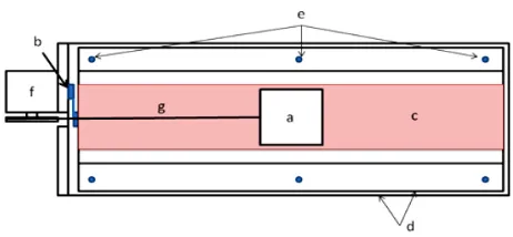
The experiment series reported in this work has been per-formed in a simple spring-block system that we have devised in order to model a seismic fault. We have included a com-plete description of this apparatus in Ref. 1. Such appara-tus is presented schematically in Fig. 1. The interfaces of interest that act as the seismic fault surfaces have been con-structed with one aluminum block which is a solid square (0.1 m (sides) and 0.025 m (high)) with a mass of 0.5 kg, supported by an aluminum plate. Both pieces have been re-covered with sandpaper of the same grade on their respective contact surfaces. The aluminum plate is sustained over a very low friction table which was constructed with a pair of glass plates with steel balls between them. The previous system is held fixed on a heavy metal frame to provide it mechanical stability. The aluminum block is pulled at constant speed of 2.22×10−4 _ms−1_{with an elastic rope (fishing line) attached}

to two series reducing system 60:1 variable speed DC motor (Baldor CD5319). We fixed a charge cell (Omega LCL) to the metal frame in order to measure the force exerted by the aluminum plate over it. That is, the charge cell acts like a bumper between the aluminum plate and the metalic frame. During the experimental run the system has succesive stick– slip events like those shown in Fig. 2.

3.

Methods

3.1. Detrended Fluctuation Analysis

In Ref. 17 Peng et al. introduced detrended fluctuation analy-sis (DFA) to detect correlations in irregular and nonstationary signals. The DFA method is based on the classical random walk variations. To illustrate DFA, we depart from an initial time seriesB(i)(of lengthN), with

Bave= 1

N

N

X

j=1

B(i).

First, this series is integrated,

y(k) =

k

X

i=1

[B(i)−Bave],

FIGURE1. Schematic top view of the experimental setup. a) Slid-ing block with sand-paper in the bottom surface, b) load cell, c) rough surface mounted in an aluminum base, d) suspension glass plates, e) steel spheres, f) DC motor, with gear mechanism, g) elas-tic rope.

FIGURE2. Time series (force as a time function) recorded with a charge cell.

after doing this, the resulting series is divided into boxes of size n. For each box, a straight line is fitted to the points,

yn(k). Next, the line points are subtracted from the integrated

series,y(k), in each box. The root mean square fluctuation of the integrated and detrended series is calculated by means of

F(n) = v u u t1

N

N

X

k=1

[y(k)−yn(k)]2, (1)

this process is taken over several scales (box sizes) to obtain a power law behaviorF(n)∝nγ_{, withγan exponent which}

reflects self-similar properties of the signal. It is known that

γ = 0.5corresponds to white noise (non correlated signal),

γ= 1corresponds1/fnoise andγ= 1.5represents a Brow-nian motion [18]. The DFA-exponentγ is related with the spectral exponent β by means of β = 2γ −1 [18], thus also with the fractal dimensionD (see next Subsection) by

γ= 3−D.

3.2. Higuchi Method

Higuchi method [19,20]. In Ref. 21 Higuchi proposed a method to calculate fractal dimension of self-affine curves in terms of the slope of the straight line that fits the length of the curve versus the time interval (the lag) in a double log plot. The method consists in considering a finite set of data taken atν1, ν2, ...νN. From this series we construct new time

series,νk

m,defined as

ν(m), ν(m+k), ν(m+ 2k), ..., ν

µ

m+ ·

N−k k

¸ ·k

¶ ;

with m= 1,2,3, ..., k. (2) where [ ] denotes Gauss’ notation, that is, the bigger integer andmandkare integers that indicate the initial time and the interval time, respectively. The length of the curveνk

m, is

defined as:

Lm(k) = 1

k

" ³[N_X−km]

i=1

|ν(m+ik)

−ν(m+ (i−1)k)|

´ _N−1 £_N−m

k

¤

k

#

(3)

and the term(N−1)/[(N−m)/k]krepresents a normaliza-tion factor. Then, the length of the curve for the time interval

kis given byhL(k)i:the average value overksetsLm(k).

Finally, ifhL(k)i ∝ k−D, then the curve is fractal with di-mensionD[21]. The fractal dimension is related to the spec-tral exponentβby means ofβ= 5−2D[21]. Note that this relationship is valid for1< D <2and1< β <3.

4.

Data Analysis

In Fig. 2 we show a segment of a typical time series of force values registred at the charge cell. In this figure we can see how seccesively the force between the rugged surfaces in-creases (with a saw profile) when the blocks sticks to the

rug-FIGURE3. Example of a typical graph of the sliding size sequence as a function of time.

FIGURE4. LogF(n)vs. lognfrom sliding size sequences for several runs.

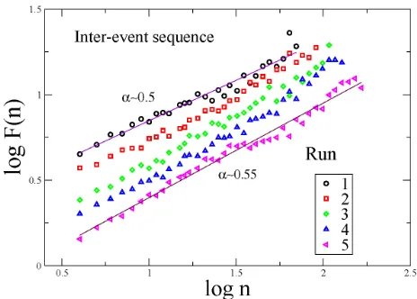
FIGURE5. LogF(n)vs. lognfrom inter-event time sequences for several runs.

ged track and abruptly decreases when the block slips. We construct the cummulative distribution of sliding eventsN(s) with amplitude larger than s, and in all experimental runs we find Gutenberg–Richter (G-R) type laws of the form

N(S > s) ∼ S−b _{(see Figs. 3, 4, 5 and 6 of Ref. 1). In}

see that for runs from 2 to 5, that is, with the aging effect of the sandpapers the DFA-exponent tends toγ ≈ 0.5, that is, a white noise with loss of correlations. The larger the wear of the asperities the larger the loss of memory in succesive slidings. This result is very consistent with real seismicity, where tipically after a great earthquake a sequence of after-shocks evidently correlated with the mainshock occurs. The big earthquakes are linked with fault interfaces dominated by big asperities. When the asperities are of small size the upper limit for the magnitude of a mainshock disminishes. For the case of the interevent times (Fig. 5) the values of the DFA-exponents go fromγ ≈ 0.5 up toγ ≈ 0.55; that is, from uncorrelated sequences to slightly persistent fluctuations, in-dicating the presence of positive correlations.

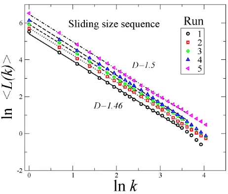
It is convenient to remark that in both cases (Fig. 4 and Fig. 5) the dynamical behavior is relatively near to uncor-related signals (white noise). For the case of the Higuchi’s method, we first integrate both the sliding size and the in-terevent time series. As we can see in Fig. 6, for the fifth run the fractal dimension isD = 1.5(Brownian noise) cor-responding to the original white noise signal which once in-tegrated gives Brownian noise. That is, a result completely consistent with γ = 0.5 for the most wore interface. For the first run D = 1.46 corresponding to a persistent se-quence of sliding sizes. If one uses the simple relation-ship α+ 1 = 3−D [22], we get α ≈ 0.54, which is in reasonable agreement with the value obtained by means of DFA (α = 0.6). In Fig. 7 we depict the log-log plot whose slope gives the Higuchi’s fractal dimension for the se-quence of interevent times. In this case, the first run leads to

D ≈ 1.5which corresponds to integrated uncorrelated fluc-tuations whereas for the fifth run, the value isD= 1.4which is also consistent with the results from DFA analysis.

FIGURE6. Log-log plot ofhL(k)ivskfor sliding size sequences. We observe that the fractal dimension decreases as the run number increases. The original series was integrated to improve the resolu-tion.

FIGURE 7. Log-log plot ofhL(k)i vsk for interevent time se-quences. The original series was integrated to improve the resolu-tion.

5.

Concluding remarks

asperities. That is the resolution of interevent times is not of good quality. In summary, by means of DFA and Higuchi’s methods we observe some of main properties of seismicity only corresponding to sliding size sequences, but for interval times our results are not clear, and asperities of bigger sizes will be necessary.

Acknowledgments

LGV and FAB thank COFA-EDI-IPN for partial financial support

1. C.A. Vargas, E. Basurto, L. Guzm´an-Vargas, and F. Angulo-Brown, Physica A 387 (2008) 3137.

2. R. Burridge and L. Knopoff, Bull. Seismol. Am. 57 (1967) 341.

3. H.J.S. Feder and J. Feder, Phys. Rev. Lett. 66 (1991) 2669.

4. P. Bak, C. Tang, and K. Wiesenfeld, Phys. Rev. Lett. 59 (1987) 381.

5. R. Geller, D.D. Jackson, Y. Kagan, and F. Mulargia, Science 275 (1977) 1616.

6. J.M. Carlson and J.S. Langer, Phys. Rev. A 40 (1989) 6470.

7. K. Ito and M. Matsuzaki, J. Geophys. Res. 95 (1990) 6853.

8. H. Nakanishi, Phys. Rev. A 41 (1990) 7086.

9. S.R. Brown, C.H. Scholz, and J.B. Rundle, Geophys. Res. Lett. 18 (1991) 215.

10. Z. Olami, H.J.S. Feder, and K. Christensen, Phys. Rev. Lett. 68 (1992) 1244.

11. K. Christensen and Z. Olami, Phys. Rev. A 46: (1992) 1829.

12. B. Barriere and D.L. Turcotte, Phys. Rev. E 49 (1994) 1151.

13. C.D. Ferguson, W. Klein and J.B. Rundle, Comp. Phys. 12 (1999) 34.

14. A. Mu˜noz-Diosdado and F. Angulo-Brown, Rev. Mex. Fis. 45 (1999) 393.

15. F. Angulo-Brown and A. Mu˜noz-Diosdado, Geophys. J. Int. 139 (1999) 410.

16. D.L. Turcotte, Rep. Prog. Phys. 62 (1999) 1377.

17. C.–K. Peng, J. Mietus, J.M. Hausdorff, S. Havlin, H.E. Stanley, and A.L. Goldberger, Phys. Rev. Lett. 70 (1993) 1343.

18. N. Iyengar, C.–K. Peng, R. Morin, A.L. Goldberger, L.A. Lip-sitz, Am. J. Physiol. 271 (1996) R1078.

19. L. Guzm´an–Vargas, and F. Angulo-Brown, Phys. Rev. A 67 (2003) 052901-1.

20. L. Guzm´an–Vargas, E. Calleja-Quevedo, and F. Angulo-Brown,

Fluctuation and Noise Letters 3 (2003) L81.

21. T. Higuchi, Physica D 31 (1988) 277; T. Higuchi, Physica D 46 (1990) 254.