A Recurrent Neural Network for Wastewater Treatment Plant
effluents’ prediction
Ivan Pisa, Ignacio Sant´ın, Jose Lopez Vicario, Antoni Morell, Ramon Vilanova,
{Ivan.Pisa, Ignacio.Santin, Jose.Vicario, Antoni.Morell, Ramon.Vilanova}@uab.cat Department of Telecommunications and Systems Engineering,
Universitat Aut`onoma de Barcelona, 08193 Bellaterra, Spain
Abstract
Wastewater Treatment Plants (WWTP) are in-dustries devoted to process water coming from cities’ sewer systems and to reduce their contami-nation. High-pollutant products are generated in the pollutant reduction processes. For this rea-son, certain limits are established and violations of them are translated into high economic punish-ments and environmental problems. In this paper data driven methods are performed to monitor the WWTP behaviour. The aim is to predict its efflu-ent concefflu-entrations in order to reduce possible vio-lations and their derived costs. To do so, an alarm generation system based on the application of Ar-tificial Neural Networks (ANNs) is proposed. The proposed system shows a good prediction accuracy (errors around 5%) and a reduced miss-detection probability (30%).
Keywords: Wastewater Treatment Plants,
Neural Networks, LSTM cells, BSM2
1
Introduction
Wastewater Treatment Plants (WWTPs) are de-voted to manage and process the residual waters coming from the cities’ sewer systems. In WWTP plants, biological and biochemical processes are applied to water to decrease the pollutants such as ammonium (SN H) and total nitrogen (SN tot) concentrations. The processes, which are highly complex, are also applied to avoid the contamina-tion of the ecosystem where treated water flows. Furthermore, there exist some limits established by law which determine the maximum concentra-tion levels of certain WWTP products. Violaconcentra-tions of these limits are translated into high economic punishments and environmental problems.
In that sense, the International Water Association (IWA) has developed a mathematical model, the Benchmark Simulation Model No.1 (BSM1) [2], which replicates the WWTP’s real behaviour. It models the biological treatment of the water based on the Activated Sludge Model No.1 (ASM1) [7]. BSM1 has been enhanced with the appearance of
the Benchmark Simulation Model No.2 (BSM2) which includes the activated sludge treatment [4]. Both, BSM2 and BSM1 models, are adopted as the evaluation scenarios of new control strategies to maintain the pollutants below the established limits.
In such a context, the appearance of Artificial Neural Networks (ANNs) [5] has arisen as a method able to model the WWTP behaviour with-out the knowledge of BSM2 and BSM1 models, they only require the WWTP’s influent and efflu-ent data [8].
For instance, ANNs are adopted to forecast or pre-dict some parameters to feed a control strategy. In that sense, Foscoliano et.al propose the adoption of RNN networks to predict the WWTP’s nutrient concentrations and then, feed a Model Predictive Control (MPC) strategy to assure that concentra-tions are under the established limits [3]. Fur-thermore, Sant´ın et.al adopt two Multilayer Per-ceptron (MLP) neural networks to predict the am-monia and total nitrogen concentrations in the ef-fluent and determine whenever a violation of their limits is likely to occur [10].
On the other hand, there are several works where ANNs have been adopted to monitor or predict some WWTPs’ parameters. For instance, in [6], the Chemical Oxygen on Demand (COD), the Sus-pended Solids (SS) and the aeration tank concen-trations (SO) are predicted by means of three dif-ferent Multilayer Perceptron (MLP) neural net-works yielding a Mean Absolute Percentage Error (MAPE) in the prediction around 4.48%.
In this work we propose a system based on ANNs to predict violations of the ammonium and to-tal nitrogen concentrations and generate an alarm to determine when the control strategy (MPC + Fuzzy Logic) has to be activated. Furthermore, the temporal behaviour and dependence between WWTP’s inputs and outputs will be modeled adopting LSTM cells. Our main contributions to the state of the art are:
• Adopt RNN and LSTM structures to deal with time series and temporal data.
• Consider online and continuous data. Thus, the time dependence is conserved and pre-dictions can be performed with information gathered in the same WWTP.
• Reduce the time between predictions. As a consequence of the adoption of continuous data, predictions are given every 15 minutes.
2
Problem Definition
The main objectives of WWTP plants is to reduce the amount of pollutant concentrations in water and return it to its natural cycle. Consequently, one of the main objectives of this work consists in the adoption of data driven methods to model the WWTPs behaviour in order to predict effluent nutrient concentrations. With these predictions, possible violations of the established effluent lim-its for such nutrients can be eliminated, therefore reducing the receiving water’s pollution and avoid-ing possible economic sanctions. The considered pollutants are the nitrogen and phosphorous.
In this work we will concentrate on the nitrogen removal. Nitrogen is considered in the form of ammonia and total nitrogen, treated with Biolog-ical WWTPs. The BiologBiolog-ical treatment is split into two processes which are known as nitrifica-tion and denitrificanitrifica-tion. The first one is in charge of transforming the ammonia into nitrate while the second converts the nitrate into nitrogen and other gaseous products [14]. These processes are modeled by the widely accepted ASM models [7], that are incorporated into the BSM2, benchmark scenario developed by the IWA [4].
Table 1: Effluent quality limits
Effluent quality limits
Variable Value
SN tot <18 mg/L
SN H <4 mg/L
For what matters to the BSM2 scenario, the es-tablished effluent limits are shown in Tab.1 where
SN totandSN H are the total nitrogen and the am-monium concentrations [4], both measured in the effluent.
3
Material & Methods
3.1 Benchmark Simulation Model No. 2
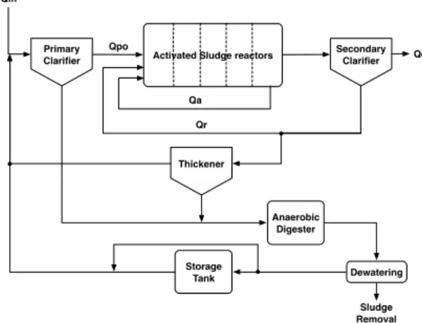
The adopted input and output data will be gener-ated through the usage of the BSM2 model, which is an enhancement of BSM1 model [2]. BSM2 is formed by two clearly differentiated sections, the
first one is in charge of the water’s biological treat-ment at the activated sludge reactors, and the sec-ond one is in charge of the sludge treatment. Wa-ter’s biological treatment is based on BSM1.
BSM1 consists in five biological reactor tanks which are connected in series. The first two tanks are anoxic tanks (they have a lack of oxygen) whereas the three remaining are aerobic. Their biological process is described in [7]. An internal recycle flow is considered from the last tank to the first one. In addition, BSM1 model considers a clarifier connected to the fifth tank’s output. This clarifier is adopted to perform the sludge sedimen-tation process following the Tak´acs model [12]. Concerning the flow rates, the plant considered in BSM2 and BSM1 models is designed consider-ing an average flow rate of 20648.36 m3/d. Each
anoxic tank has a volume of 1500 m3 and each
aerobic tank has a volume of 300 m3. Thus, the retention time considering the total volume of the tanks and the flow rate is about 14h.
Activated Sludge reactors Primary
Clarifier
Secondary Clarifier Qin
Qe
Qa
Qr Qpo
Thickener
Anaerobic Digester
Dewatering
Sludge Removal Storage
Tank
Figure 1: BSM2 model for a plant structure
BSM2 adds different elements whose purpose are to treat the sludge. In such a context, a primary clarifier, a thickener for the sludge wasted in the secondary clarifier, an anaerobic digester to treat the wasted solids and a dewatering module are added to the BSM1 model as it is shown in Fig.1. In it, the different flow rates are specified: Qin corresponds to the input flow,Qpo is the primary clarifier overflow, Qa is the internal recycle flow rate, Qr is the sludge internal recycle flow rate and finallyQe is the effluent flow rate.
influent is adopted. Nonetheless, the BSM2 sim-ulation protocol specifies that only results from days 245 to 609 have to be taken into account for plant evaluation. The BSM2 effluent file is gener-ated adopting the plant structure and the control strategies adopted. It gathers information about the nutrient concentrations and the effluent rate among others with a sampling time of 15 minutes. Thus, four consecutive samples correspond to one hour of WWTP’s operation.
3.2 Artificial Neural Networks
The ability of ANNs to model non-linear sys-tem has motivated us to adopt them as the main method to generate WWTPs’ effluent predictions. ANNs structures consist in a set of layers [5]. Each layer presents an amount of hidden neurons which are characterized by the activation function they adopt. In this context, activation functions are ap-plied to obtain the neuron output in terms of the input. Layers are connected to each other through weights and biases.
ANN’s model is generated by means of an iterative process called training process where the values of the weights and biases are optimized. In that sense, weights and biases are modified iteratively taking into account the input data and the gen-erated outcomes. For this reason, a large dataset of input and output values is required. Moreover, this dataset will be split in three subsets following the next otherwise usual distribution: 70%, the training dataset devoted to perform the training process; 15%, the validation dataset to validate the training and to see if overfitting is committed; and 15%, the test dataset to see the performance of the network with new data.
The values of weights and biases are optimized taking into account a cost function. It corresponds to a measurement of how well is predicting or clas-sifying the ANN. For this reason, it is selected according to the purpose of the neural network. Since this work is focused on regression purposes, the Mean Square Error (MSE) function (Eq. 1) is adopted,
J(θ) = 1
N
N
X
i
(yi−ybi)
2 (1)
where N is the number of examples, yi is the de-sired output,ybi corresponds to the ANN’s predic-tion andθcorresponds to the weights of the neural network.
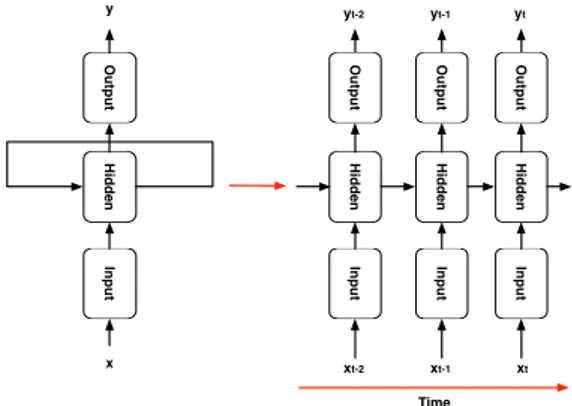
In this work, predictions are performed adopting LSTM cells which are a type of Recurrent Neu-ral Networks (RNNs). RNNs are ANNs wherein
connections between hidden neurons form a di-rected cycle (unfolding process is observable in Fig.2). This means that the hidden state of the neural network is adopted to give some extra in-formation about the dynamics of the inputs. In addition, RNNs are widely known due to its be-haviour modeling sequences and continuous sig-nals such as text or voice [13]. In addition, they are also recommended due to their ability model-ing systems with non-linear dynamics [5, Chapter 12]. Furthermore, RNN structures have yielded very good results dealing with time series and se-quence recognition problems [11]. This motivates us to consider them in our problem, the signals we are dealing with are continuous in time with a strongly dependence between inputs and outputs.
O
u
tp
u
t
H
id
d
e
n
In
p
u
t
O
u
tp
u
t
H
id
d
e
n
In
p
u
t
O
u
tp
u
t
H
id
d
e
n
In
p
u
t
O
u
tp
u
t
H
id
d
e
n
In
p
u
t
Time x
y
xt-2
yt-2
xt-1 xt
yt-1 yt
Figure 2: Unfolding process for RNN Network for Time Series
Training process is performed adopting the back-propagation through time (BPTT) algorithm, which is based on the iterative update of the net-work weights towards the opposite of the gradi-ent of the loss function w.r.t the weights. How-ever, back propagation algorithm has some draw-backs when it is adopted in the training process of RNNs, due to the well-known exploding or van-ishing gradients problem [1]. In that sense, gated networks such as the LSTM cell approach (See Fig.3) appeared as a promising alternate struc-ture to alleviate this problem. They replace the hidden neuron by a memory cell with three gates, the forget, the input and the output gates. The forget gate can reset the memory cell which will be fulfilled with the information coming from the input gate. The output gate will determine if the output will influence on other cells [5, Chapter 10].
x +
x
x Tanh
Tanh σ
σ σ
xt
ht
ct
ht ct-1
ht-1
ft it c’t ot
Figure 3: LSTM Cell
starts to drop and become worse than before. L2 consists in adding extra penalty to the weights optimization. As a consequence, it is harder for the network to match the training examples as for weights cannot grow without penalty [5, Chapter 7]. DropOut consists in the application of “keep probabilities” at the output of the hidden neurons in a layer, i.e, neurons’ output are activated fol-lowing the given “keep probabilities”. It can be interpreted as performing a mixture of models as far as different networks are considered (depend-ing on the set of active neurons). This leads to a generalization of the weights.
4
Effluent nutrient violation’s
prediction in WWTP’s
As it has been stated in previously sections, the main purpose of WWTP plants is to decrease the pollutant levels and therefore avoid the contam-ination of the receiver waters. Thus, the efflu-ent’s levels are limited and therefore any viola-tion of them incur into an economical sancviola-tion to the plant. In addition, there are several control strategies proposed in the literature whose objec-tives are to reduce the levels of effluent products. However, the application of control strategies can involve an increase of the plant’s operational cost.
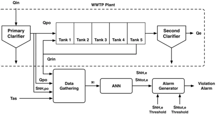
In such a context, we propose the ANN-based Ef-fluent Violation Prediction (AEVP) system (See Fig.4) which objective is to predict possible viola-tions of WWTP’s effluent limits, thereby the con-trol strategies can be applied only when they are required and also the effluent limit violations can be avoided. The system consists in three differ-ent stages: the Gathering Information, the ANN (based on RNNs) and the Alarm Generation sub-systems. Their purpose is to gather the online information from the WWTP plant, preprocess it and then perform predictions of the effluent levels by means of ANNs. Predictions will be contrasted
with the limits (See Tab.1).
4.1 Prediction Objective & Input Data
ANNs will be adopted in the AEVP system to model the WWTP’s dynamics and behaviours in an attempt to overcome the use of the high com-plexity deterministic models considered in BSM2 [4]. Generated models will be used to predict the effluent concentrations of ammonium and total ni-trogen (SN H,eandSN tot,e). These predictions will determine when the effluent concentration limits (See Table 1) will be violated or, more precisely, they are at risk of being violated. The ANN will be trained taking into account a subset of the WWTP influent data and its correspondent outputs.
In this work, the inputs gathered by the Gather-ing Information subsystem consist in online data given by sensors placed in the WWTP plant. In that sense, predictions can be performed directly without the necessity of laboratory analysis as it happens with offline data [15]. The influent subset corresponds to:
• SN H,po: Ammonium concentration of the pri-mary clarifier
• Qpo: Overflow rate of the primary clarifier
• SN H,po·Qpo
• Qrin: internal recycle flow rate
• Tas: Temperature
SN H,po is considered because it is one of the pol-lutants with the higher influence on the total fi-nal nitrogen concentration (SN tot,e). It not only increases the concentration of ammonium in the effluent, but it also affects the nitrification pro-cess and consequently the resultingSN tot,e. Tasis added due to its influence in the nitrification and denitrification processes performed in the tanks of the BSM2 model. The product between SN H,po andQpo, is also considered due to its appearance in the general mass balancing equations of the ASM1 model [7]. The output data has been gath-ered from BSM2 models with the MPC + Fuzzy Logic strategy defined in [9]. Data has been nor-malized to zero mean and unit variance to reduce the range of input values.
Primary Clarifier
Qpo
Tank 1 Tank 2 Tank 3 Tank 4 Tank 5
Qe
Second Clarifier
Qin
Data
Gathering ANN
Alarm Generator Qpo
SNH,po Qrin
Tas
xt
SNH,e
SNtot,e WWTP Plant
Violation Alarm
SNH,e Threshold
SNtot,e Threshold
Figure 4: AEVP system to predict WWTP’s effluent levels and determine if violations will be committed
horizon (PH), where PH is defined as the amount of time the prediction can be given in advance. Their configurations are the following ones:
• Window Length (WL): A WL of 10 hours (40 samples) is considered. The input data not only corresponds to the values seen at each sampling time, but also to those seen previ-ously. Thus, when the sliding window slides the oldest input data is discarded and the newest one is considered.
• Prediction Horizon (PH): A PH of 4 hours (16 samples) is considered. Output data cor-responds to the effluent concentrations of to-tal nitrogen (SN tot,e) and ammonium (SN H,e) which will be observable in four hours.
The adoption of these WL and PH configurations are motivated by the fact that the retention time of the BSM2 model is estimated of 14 hours. Thus, the first input value of the sliding window is sup-posed to generate the output prediction after 14 hours. For example, if it is gathered at 00:00h, the generated output is supposed to come out of the WWTP at 14:00h. Thus, if a sliding window of 10h is considered, a PH of 4h is needed (See Fig.5).
14h00 4 hours
0h00 10h00
Data
Figure 5: Sliding window example
4.2 ANN’s prediction structures
Predictions are performed according to the ANN subsystem which is in charge of taking the input values given by the Gathering Information subsys-tem and predicting the effluent concentration lev-els. Those correspond to the ammonium (SN H,e)
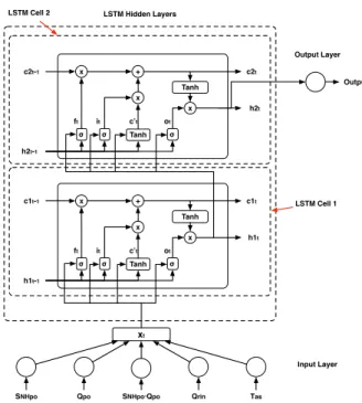
and total nitrogen (SN tot,e) concentrations. In that sense, LSTM Structures are adopted as a prediction approach: five LSTM-based prediction structures, three for the effluent ammonium con-centration (SN H,e) and two for the total nitro-gen effluent concentration (SN tot,e). The proposed LSTM-based prediction structures are:
• Ammonium Prediction Structure (APS): The APS structure is formed by an input layer of 5 input neurons connected to the LSTM hidden layers (one LSTM1), two (APS-LSTM2), or three (APS-LSTM3)) of 50 den units each LSTM hidden layer. Each hid-den layer contains one LSTM cell. The last hidden layer is connected to an output layer formed by one output neuron with a linear activation function.
• Total Nitrogen Prediction Structure (TNPS): The TNPS structure is formed by an input layer of 5 input neurons connected to the LSTM hidden layers (one (TNPS-LSTM1) or two (TNPS-LSTM2)) of 10 hidden units each LSTM hidden layer. The last LSTM hidden layer is connected to an output layer with one output neuron adopting the linear acti-vation function. TNPS-LSTM2 is presented in Fig.6.
4.3 Prediction & Alarm Generation Results
x +
x x Tanh
Tanh σ σ
σ
c1t
h1t
c1t-1
h1t-1
ft it c’t ot
x +
x x Tanh
Tanh σ σ
σ
c2t
h2t
c2t-1
h2t-1
ft it c’t ot
LSTM Hidden Layers
LSTM Cell 1
SNHpo Qpo SNHpo·Qpo Qrin Tas
Input Layer
xt
Output Layer
Output LSTM Cell 2
Figure 6: Total Nitrogen Prediction Structure (TNPS-LSTM2) - 2 LSTM hidden layers with 10 hidden units per LSTM cell
is defined as the probability of predicting an inex-istent limit violation whereas Pmiss is defined as the probability of missing a real limit violation.
The MAPE criteria is computed as follows:
M AP E= 1
N ·
N
X
i=1
yi−ybi
yi
·100 (2)
where MAPE represents the percentage of error committed in the predictions with respect to the real output value. The main point is not to pre-dict the exact behaviour of the WWTP plant with high precision but to detect the possible effluent violations.
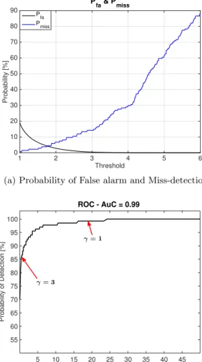
Finally, predictions are adopted to feed the Alarm Generation subsystem. It will compare the pre-dicted value with the effluent limits. Thus, prob-abilities of false alarm (Pf a) and miss-detection (Pmiss) make sense in the evaluation of the Alarm Generation Subsystem’s results. Pmiss and Pf a are defined as:
Pmiss=P(ybi< γ|yi≥γ) (3)
Pf a =P(ybi≥γ|yi< γ) (4)
where ybi corresponds to theith value of the pre-dictions, yi represents the ith real output and γ consists in the effluent limit or threshold. The
ef-fluent limits adopted to determine if there exists an alarm are the ones shown in Tab.1.
Table 2: Performance of ANN effluent concentra-tion predicconcentra-tion
ANNs prediction performance
Ammonium in the effluent -SN H,e Structure MAPE [%] Pf a [%] Pmiss [%]
APS-LSTM1 8.08 0.01 41.04
APS-LSTM2 7.93 0.03 29.85
APS-LSTM3 7.87 0.04 35.07
Total Nitrogen in the effluent - SN tot,e Structure MAPE [%] Pf a [%] Pmiss [%]
TNPS-LSTM1 4.84 0.45 39.57
TNPS-LSTM2 4.69 0.44 31.75
Performance of the ammonium and total nitrogen prediction structures is shown in Tab.2. MAPE criteria shows that the percentage of the error committed in the prediction is lower than a 10% for SN H,e prediction structures. In such a con-text, one can observe that the lowest MAPE is given by the APS with 2 hidden layers structure showing aPmiss of 29.85%. However, there is an exception with the APS with 3 hidden layers. It shows a lower MAPE but a higherPmissthan the APS with 2 hidden layers. This effect is moti-vated by the fact that APS with 3 HL is affected by overfitting. Overfitting is defined as the effect where the ANN’s model is not able to generalize. It is produced when the model is over trained. Concerning theSN tot,e prediction structures, one can observe that MAPE criteria shows that the error committed is lower. In terms of Pmiss, the same tendency as inSN H,eis observable. Finally, it can be stated that there exists a correlation be-tween the MAPE and thePmisscriteria, when the former decreases the latter does so. Performed predictions are observable in Fig.7. Finally, APS and TNPS with 2HL structures (APS-LSTM2 & TNPS-LSTM2) are the ones showing the best per-formance in terms of MAPE &Pmiss (See Tab.2).
In terms of the predictions’ accuracy, miss-detection can be reduced by adjusting violation threshold, which could lead to an increase of the false alarm probability. In other words, theSN H,e andSN tot,elimits of the alarm generation process can be reduced but maintaining the real limits to those shown in Tab.1. Thus, the Receiver Op-erating Characteristic (ROC), Pf a and Pdetection (beingPdetection= 1−Pmiss), can be obtained as a function of the threshold of the alarm genera-tion system. By modifying the threshold, one can adjust Pf a and Pmiss. For instance, ROC curve shows that a γ = 3 mg/L yields aPf a = 0.44% and a Pdetection = 85.82% whereas, if a γ = 1
No-Time (Days)
555 556 557 558 559 560 561 562
SNH,e
(mg/L)
0 1 2 3 4 5 6
S
NH,e vs Time
Real Predicted SNH,e limit
(a) NH concentration’s prediction
Time (Days)
555 556 557 558 559 560 561 562
SNtot,e
(mg/L)
4 6 8 10 12 14 16 18 20 22 24
S
Ntot,e vs Time
Real Predicted S
Ntot,e limit
(b) Ntot concentration’s prediction
Figure 7: Real and predicted NH and Ntot con-centrations in the effluent - APS-LSTM2 & TNPS-LSTM2 structures are adopted
tice that, curve of ROC showing an Area under the Curve (AuC) of 0.99 is obtained (a value equal to 1 represents perfect performance). Pf a vs. Pmiss for APS-LSTM2 configuration is shown in Fig.8.
5
Conclusion
In this paper, the application of neural networks to predict SN H,e and SN tot,e in WWTP’s efflu-ent is presefflu-ented. Their main goal is to determine when effluent concentrations are prone to exceed the established limits. In that sense a system to generate alarms has been proposed. Its purpose is to predict future WWTP’s concentration values adopting RNN in order to reduce the number of violations and the derived costs.
Predictions are performed adopting two RNN-based LSTM structures, one for SN H,e and an-other for SN tot,e. They will determine when ef-fluent concentrations limits are at risk of being
Threshold
1 2 3 4 5 6
Probability [%]
0 10 20 30 40 50 60 70 80 90
P
fa & Pmiss
P fa Pmiss
(a) Probability of False alarm and Miss-detection
5 10 15 20 25 30 35 40 45
Probability of False Alarm [%] 55
60 65 70 75 80 85 90 95 100
Probability of Detection [%]
ROC - AuC = 0.99
(b) Receiver Operating Characteristic (ROC)
Figure 8: Pf a vs. Pmiss (a) and ROC (b) for APS-LSTM2. ROC shows the trade-off between
Pf a andPdetection. Pdetection= 1−Pmiss.
violated and consequently when an alarm has to be generated. Thereby control strategies will be executed when alarms are generated. This can be translated in a reduction of the operation cost of the plant and also the violations of effluents’ lim-its.
Results show a miss-detection probability (Pmiss) around 30% for both cases. In addition, low pre-diction errors (low MAPE) are achieved. More-over, the system considers the option to mod-ify alarm thresholds in order to adjust the miss-detection probability at the expense of a higher false alarm. ROC curve has been computed show-ing an Area under the Curve of 0.99 (1 is perfect performance).
Acknowledgement
Com-petitiveness program under MINECO/FEDER grant DPI2016-77271-R and also from La Secre-taria d’Universitats i Recerca del Departament d’Empresa i Coneixement de la Generalitat de Catalunya i del Fons Social Europeu under FI grant. Authors belong to the Recognized Con-solidated Research group SGR 1202 and to the Recognized Emergent Research group SGR 1670 by the Catalan Government.
References
[1] Y. Bengio, P. Simard, and P. Frasconi, “Learning Long-Term Dependencies with Gradient Descent is Difficult,” IEEE Trans-actions on Neural Networks, vol. 5, no. 2, pp. 157–166, mar 1994.
[2] J. B. Copp, The cost simulation benchmark: Description and Simulator Manual (cost ac-tion 624 and actac-tion 682). Luxembourg: Of-fice for Official Publications of the European Union, 2002.
[3] C. Foscoliano, S. Del Vigo, M. Mulas, and S. Tronci, “Predictive control of an acti-vated sludge process for long term opera-tion,” Chemical Engineering Journal, vol. 304, pp. 1031–1044, 2016.
[4] K. V. Gernaey, U. Jeppsson, P. A. Vanrol-leghem, and J. B. Copp, Benchmarking of control strategies for wastewater treatment plants. Scientific and Technical Report No.23. London, UK: IWA Publishing, 2014.
[5] I. Goodfellow, Y. Bengio, and A. Courville, Deep Learning. MIT Press, 2016.
[6] D. G¨u¸cl¨u and S¸. Dursun, “Artificial neural network modelling of a large-scale wastewater treatment plant operation,” Bioprocess and Biosystems Engineering, vol. 33, no. 9, pp. 1051–1058, 2010.
[7] M. Henze, L. Grady Jr, W. Gujer, G. V. R Marais, and T. Matsuo, “Activated sludge model no 1,” Scientific and Technical Report No.1, vol. 29, 01 1987.
[8] H. S. Ou, C. H. Wei, H. Z. Wu, C. H. Mo, and B. Y. He, “Sequential dynamic artifi-cial neural network modeling of a full-scale coking wastewater treatment plant with flu-idized bed reactors,” Environmental Science and Pollution Research, vol. 22, no. 20, pp. 15 910–15 919, 2015.
[9] I. Sant´ın, C. Pedret, and R. Vilanova, “Fuzzy Control and Model Predictive Control Con-figurations for Effluent Violations Removal
in Wastewater Treatment Plants,”Industrial and Engineering Chemistry Research, vol. 54, no. 10, pp. 2763–2775, mar 2015.
[10] I. Sant´ın, C. Pedret, R. Vilanova, and M. Meneses, “Advanced decision control sys-tem for effluent violations removal in wastew-ater treatment plants,” Control Engineering Practice, vol. 49, no. 2, pp. 60–75, 2016.
[11] B. Shi, X. Bai, and C. Yao, “An End-to-End Trainable Neural Network for Image-Based Sequence Recognition and Its Application to Scene Text Recognition,” IEEE Transac-tions on Pattern Analysis and Machine In-telligence, vol. 39, no. 11, pp. 2298–2304, nov 2017.
[12] I. Tak´acs, G. G. Patry, and D. Nolasco, “A dynamic model of the clarification-thickening process,”Water Research, vol. 25, no. 10, pp. 1263–1271, 1991.
[13] N. Tax, I. Verenich, M. La Rosa, and M. Du-mas, “Predictive business process monitor-ing with LSTM neural networks,” inLecture Notes in Computer Science (including sub-series Lecture Notes in Artificial Intelligence and Lecture Notes in Bioinformatics), vol. 10253 LNCS. Springer, Cham, jun 2017, pp. 477–492.
[14] Z. Yang, PY and Zhang, “Nitrification and denitrification in the wastewater treatment system,” in Traditional technology for envi-ronmental conservation and sustainable de-velopment in the asian-pacific region, 1995, pp. 145–158.
[15] L. J. Zhang, N. Li, J. J. Zhang, and X. Y. Tian, “Application of neural network in mod-eling of activated sludge wastewater treat-ment process,” in 2017 36th Chinese Con-trol Conference (CCC). IEEE, jul 2017, pp. 4556–4561.
c
2018 by the authors.
Submitted for possible
open access publication
under the terms and conditions of the Creative
Commons Attribution CC-BY-NC 3.0 license