Informality in the City: a Theoretical Analysis

(1)

Informality in the City: a

Theoretical Analysis

Héctor Mauricio Posada Duque

(2)

Informality in the City: a Theoretical Analysis

Doctoral Thesis

Supervisors

Ana Isabel Moreno Monroy, Ph. D.

Juan Carlos Guataquí Roa, Ph. D.

Jury:

Ciro Biderman, Ph.D.

Ana Maria Diaz Escobar, Ph.D.

Juan Daniel Oviedo Arango, Ph.D.

DEPARTMENT OF ECONOMICS

UNIVERSIDAD COLEGIO MAYOR DE NUESTRA

SEÑORA DEL ROSARIO

(3)

(4)

List of Figures

Figure 1. Land market equilibrium at distance x to the CBD ... 28

Figure 2. Urban land use equilibrium (The segregated city) ... 31

Figure 3. Effects of decentralization on the urban land market ... 39

Figure 4. Initial effects of changes in the public infrastructure or the taxes on the land market ... 42

Figure 5. Initial effects of changes in the probability of detection on the land market ... 44

Figure 6. Effects of a higher decentralization of the informal sector ... 61

Figure 7. Effects of a rise in the commuting cost ... 62

Figure 8. Effects of a decrease in the provision of public infrastructure (or an increase in the tax level charged to formal land developers) ... 63

Figure 9. Informality rate vs. Commuting costs, and Total welfare vs. Commuting costs ... 66

Figure 10. Informality rate vs. Entry costs, and Total welfare vs. Entry costs ... 67

Figure 11. Informality rate vs. Bargaining power, and Total welfare vs. Bargaining power ... 68

Figure 12. Informality rate vs. Decentralization, and Total welfare vs. Decentralization ... 69

Figure 13. Urban land use equilibrium (the segregated city) ... 81

Figure 14. a: Total welfare vs Hiring costs. b: Informality rate vs Hiring costs ... 96

Figure 15. a: Total welfare vs Public resources. b: Informality rate vs Public resources ... 96

Figure 16. a: Total welfare vs Bargaining power. b: Informality rate vs Bargaining power ... 97

Figure 17. Housing rents in equilibrium (The segregated city) ... 116

Figure 18. Land market equilibrium at distance x to the CBD ... 119

Figure 19. Effects of a rise in the distance to the CBD ... 120

Figure 20. Effects of changes in the public infrastructure or the taxes ... 127

Figure 21. Effects of changes in the probability of detection ... 128

Figure 22. Endogenous spatial patterns of the infrastructure and the enforcement ... 132

List of Tables

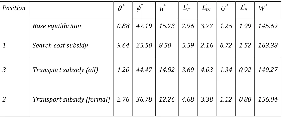
Table 1. Policy efficiency comparison ... 55

Table 2. Parameter values ... 93

(8)

(9)

Acknowledgments

(10)

(11)

Introduction

Informal labor and city structure

The informal sector occupies a significant portion of the labor market in cities in Latin America. According to recent estimates, the informal sector absorbs 57% of total workforce in the city of Bogotá, 50% in Medellin, 57% in Lima and 45% in Buenos Aires (Galvis, 2012; CNTPE, 2008; MTEySS, 2007). Part of the existing literature (Lewis, 1954; Harris and Todaro, 1970; Piore, 1980) interpretsthe informal sector as a residual sector or a buffer where rural-urban migrants queue for formal jobs. Under this view, the informal sector emerges because the inability of the modern (formal) sector to absorb the available labor supply. This inability in turn is explained by typical conditions present in markets of developing economies such as the lack of human and physical capital, the abundance of unskilled labor and the concentrated market structures, among others. Another important part of the literature (Maloney, 2004; Loayza, 1996; Rauch, 1991; Mejía and Posada, 2007) analyzes the causes of labor informality focusing on institutional reasons, and usually interprets the informal sector as a micro-entrepreneurial unregulated sector that offers intrinsic benefits, so that being informal is, to some extent, a matter of choice (Albrecht, et al., 2009).

The factors that drive economic development and institutional reforms are defined at the national or federal level and can only partly explain the incidence and persistence of urban labor informality1_{. Another set of determinants, which has not been yet extensively explored} in the theoretical literature, comes from the characteristic of cities in which informal workers reside.The existence of urban and regional labor markets is a well-established fact (Zenou, 2009). In Colombia, for example, there is considerable evidence of regional segmentation (Galvis, 2010; Mesa, et al., 2008; Ortiz, et al., 2009) which means that workers and firms interact in much smaller markets than the national market. Because of this, local factors that define the particular structure of Latin America cities (such as transport systems, workers and firms locations, and rural urban migration) can have a deep impact on urban informal labor and vice versa.

(12)

Latin American cities display high levels of spatial segregation, usually in the form of large peripheral belts where there is concentration of low-income population, poor infrastructure provision, and difficult access to city centers (Bocarejo and Portilla, 2011; ONU-HABITAT, 2012; Secretaría Distrital de Planeación, 2013). In cities like Bogotá this segregation pattern is extended to the labor market. Informal workers live in the south and southeast of the city (Montoya, 2014), in zones that are far of central areas where formal jobs are generated (Bocarejo and Portilla, 2011). These zones are also characterized by the low quality both in the road network and the public transport system and as a result, periphery inhabitants make less than 1.5 trips per day, almost half than the high-income workers (Bocarejo and Oviedo, 2012). Additionally, informal jobs tend to be less centralized than the formal (Hernández and Gutiérrez, 2011, Gutierrez, 2011), reflecting that part of the informal economic activity is carried out inside the house or in the public space.

The first two chapters of this dissertation study how the particular structure of Latin America cities can affect the size of the informal sector. The first chapter builds a monocentric city model with a labor market characterized by search frictions and the presence of an informal sector. We assume that formal workers commute on a daily basis to the city center where formal economic activity is centralized, whereas informal workers commute less often and undertake some of their productive activities at home. Because of this, informal workers end up living on the periphery. We also assume that there is presence of informal housing. We show that, in order to induce workers to accept a job in the formal sector, formal firms must compensate them with the income that they could have obtained in the informal sector. Part of this income is the commuting cost savings obtained by the informal worker by commuting less often to the city center. The model shows that both a higher decentralization of informal jobs and a higher proportion of informal housing result in a higher informality rate in the labor market (informality rate from now on). This is because both situations increase the commuting cost savings and force formal firms to pay a larger compensation.

The model is extended by introducing rural-urban migration.2_{As before, a higher} decentralization leads to a higher informality rate. This, in turn, pushes the expected income in the city downwards and reduces incentives for rural workers to migrate. However,

2_{In Latin America rural-urban migration has explained 30% of urban growth between 1980 and 2010 (CEPAL,}

(13)

surprisingly, rural urban migration increases. This is because a higher decentralization relaxes the competition for land near the city center which in turn reduces urban costs for all urban residents and effectively increases the expected income in the city. Finally, we use the extended model to compare the impact of search costs and transport policies on labor informality and welfare. The results show that an entry-cost subsidy has a higher impact on the informality rate than transport policies. This happens for two reasons. First, an entry-cost subsidy stimulates formal employment creation directly and indirectly (through a reduction in wages), while transport policies only affect formal employment creation indirectly. Second, the entry-cost subsidy affects rural-urban migration only through its effect on formal employment creation, while transport subsidies have an additional effect reducing urban costs, which ultimately lead to higher rural-urban migration and a higher saturation of the labor market. In other words, the Todaro paradox is more likely to happen when transport policies are in place.

(14)

Informal housing and city structure

Cities in Latin America are often characterized by fast spatial expansion (Inostroza, et al., 2013), low buildings height and by peripheries where precarious short buildings concentrate (ONU-HABITAT, 2012; UN-HABITAT, 2010). On the explanation of these patterns, some authors have stressed the role of rural-urban migration under high unemployment, as the main force behind the emergence of the periphery and the rapid expansion of the city (Harris and Todaro, 1970; Zenou, 2011), and others have focused on the role of the migration under agglomeration economies, in turning cities into megacities (Krugman, 1991). However, less attention has been paid to the role of informal housing. If we consider slum settlements and durable self-constructions (that avoid taxes and urban standards) as informal constructions, the informal housing sector accounts, at least, for 25% of the housing market in Latin America.3_{Therefore, the informal housing sector occupies large extensions of urban land that} could have been used by the formal sector, affecting the land market (Smolka and Biderman, 2011), the productivity in the housing industry, and finally the shape and the spatial structure of the city.

The previous theoretical literature on the economics of the informal housing sector has focused on the study of slums, emphasizing on issues such as illegal dwelling, or income differences combined with land regulations. For example, Jimenez (1985) and Brueckner and Selod (2009) study the economics of squatter settlements. Da Mata (2013) models slum growth on Brazil, focusing on the role of lack of property rights, while Heikkila and Lin (2013) study the implications of minimum lot size restrictions and the income differentials in the magnitude of slums. However, there is not a systematic approach that closely relates informal housing with the city structure. In particular, little is known about how land allocated to informal constructions changes with distance to the city center, how informal constructions can be compared with formal constructions, and how informality affects the size and tallness of the city.

The third chapter of this dissertation study how the structure of Latin American cities can be affected by (and can affect) the informal housing sector. More specifically, this chapter develops a monocentric city model with a formal and an informal sector in the housing

(15)

(16)

Chapter one

Informal labor, city structure, and rural urban

migration

4

1.1. Introduction

One of the most remarkable features of cities in Latin America is the existence and persistence of an informal sector in the labor market (Maloney, 2004; Mejía and Posada, 2007). In its most common form, informal employment refers to the case of workers who are not reported as such by their employers to the corresponding national authorities (e.g., they do not have a signed labor card). This implies that the informal sector is an unregulated sector (Albrecht, et al., 2009), where workers usually receive lower wages, do not pay taxes, do not contribute to social security system, have no record of job experience or opportunities for advancement, and have more difficulties accessing credit (Perry, et al., 2007). For the economy at large, the existence of informal employment implies losses, not only in tax revenues and a heavy social protection burden, but also in terms of productivity.

Most of the existing literature analyzing the causes of urban informality has focused on institutional reasons. There is some evidence indicating that over-regulation and red tape, a dual social security system, and lack of labor regulation enforcement all lead to higher informality rates (Perry, et al., 2007; Ferreira and Robalino, 2011). These aspects, which depend on institutional reforms at the national or federal level, can only partly explain the incidence and persistence of urban informality. Another important set of determinants, which has not been yet extensively explored in the literature, comes from the characteristic of cities in which informal workers reside.

4_{I would like to thank Ana Isabel Moreno-Monroy, Juan Carlos Guataqui, and the participants of seminars at}

(17)

Latin American cities show spatial segregation, usually in the form of large peripheral belts where there is concentration of low income population, poor infrastructure provision, and difficult access to city centers (Bocarejo and Portilla, 2011; ONU-HABITAT, 2012; Secretaría Distrital de Planeación, 2013). This segregation pattern also can be seen in the labor market. In Bogotá, for example, informal workers are concentrated in the south and southeast of the city (Montoya, 2014) where they face long distances to the city centers and the low quality both in the road network and the public transport system (Bocarejo and Portilla, 2011). All this means that periphery inhabitants experience very high costs in terms of money, time and energy when commuting to the central areas (ONU-HABITAT, 2012), where formal employment is mostly generated (Hernández and Gutiérrez, 2011; Gutiérrez, 2011). As a consequence, they commute less than the high income population.5_{Periphery inhabitants may} be reluctant to take on a formal job because it implies a disproportionate increase in commuting costs. This is even more likely if informal employment is less centralized than formal employment. This is precisely the case in Bogotá (Hernández and Gutiérrez, 2011; Gutiérrez, 2011). Additionally, following the predictions of the Spatial Mismatch Literature, in a context of high segregation, the residents of the periphery may not get enough information about formal job opportunities, or could be discriminated by formal employment based on their place of residency (Ihlanfeldt and Sjoquist, 1998).

On the other hand, the pervasiveness of informal constructions in Latin American cities is a well known fact (ONU-HABITAT 2012). The proliferation of informal constructions is partly responsible for the fast sprawling experienced by Latin American cities, especially in the last 3 decades (Urban Age Program, 2009). New informal settlements have sprung out in the fringes of cities since the start of the industrialization process experienced by the region. The result of this continuous urban expansion is the consolidation of the peripheral belts. Although informal housing and informal employment are salient features of Latin American cities, there is not much available evidence on the relationship between the two.

The aim of this paper is to study the relationship between informal employment and city structure. We develop a spatial search model which includes relevant features of informal employment and informal housing in Latin America. Starting with a linear city with a unique

5_{In Bogotá, for instance, poorer workers make on average 1.5 trips a day, less than the average of the rich}

(18)

Central Business District (CBD) where all formal firms locate, we assume that informal workers do not pay taxes, are self-employed, and receive a transfer from the government in the form of subsidized healthcare. In this way, the informal sector can be considered as a micro-entrepreneurial unregulated sector that offers intrinsic benefits. This captures the view, relevant for the Latin America case, that being informal employed is, to some extent, a matter of choice (Albrecht, et al., 2009; Maloney, 2004, Perry, et al., 2007). Unlike formal workers, informal workers can undertake part of their productive activities at home, and consequently commute with less frequency to the CBD. As a result, informal workers live in the periphery. This structure reflects, first, that informal employment is more decentralized than formal employment and, second, the existence of segregation.

Next, following Posada (2015), we introduce informal housing in the urban land market. We assume two types of developers, formal and informal. Both types produce a homogeneous good (interior space) using urban land. Unlike formal developers, informal developers, while producing interior space, evade taxes, access public infrastructure in an irregular way, and use inefficient building techniques. They also assume a certain risk of being detected and punished. These assumptions aim to capture the most important features of informal land markets in Latin America.6_{Within this framework, we study the mechanisms relating} informal housing and informal employment. The model allows us to draw predictions relating to the provision of basic public infrastructure, commuting costs and the probability of detection on both the incidence of informal housing and informal employment.

The results show that in order to induce workers to accept a job in the formal sector, formal firms must compensate them with the expected income obtained outside the formal sector. This expected income is a weighted sum of the income obtained as an unemployed (e.g. unemployment insurance) and the income obtained as an informal worker. Part of this income is the commuting cost saving obtained by the informal worker by commuting less often to the city center.7_{We demonstrate how higher informal job decentralization, a higher}

6According to Smolka and Biderman , pag. 6: )nformality can open a gap for arbitrage, allowing infor_mal

developers to reap higher profits than formal developers because they avoid paying license fees and taxes, only partially provide infrastructure and services, devote smaller percentages of land to public uses, and offer below-minimum-size lots. These incentives stimulate supply of informal developments.

7_{This spatial compensation is different from the spatial compensation that arises when the commuting frequency}

(19)

commuting cost, and a higher proportion of informal housing (as a result of lower infrastructure provision, or a lower probability of detection) all result in a higher informality rate. This is because all these situations increase the benefits of not commuting frequently to the CBD, and consequently increase the spatial compensation that formal firms have to offer as part of the formal wage.

Besides high levels of labor and housing informality, Latin American cities have showed large rural-urban migration flows. For instance, rural-urban migration has explained 30% of urban growth between 1980 and 2010 (CEPAL, 2012). Such migration has raised important questions because it has occurred precisely in cities where poverty, unemployment and informality are present. This is the basis of the seminal work of Harris and Todaro (1970), which explains how migration occurs under a persistent urban unemployment. Harris and Todaro recognized that when rural workers migrate to the city, they accept the possibility of being unemployed to get an urban job later. That is, Harris and Todaro recognized that decisions to migrate are based on differences between expected urban income and rural income. In their model, the equilibrating mechanism is the rate of urban unemployment. As the urban population increases the unemployment rate also increases. As a result, the expected income in the city decreases, reducing the incentives to migrate.

The Harris-Todaro model has been extended in many ways8_{, and some of these extensions} have been useful to understand the relationship between city structure and migration. For example, Brueckner and Zenou (1999) and Brueckner and Kim (2001) have incorporated an urban land market into the standard Harris-Todaro model and have showed that besides the unemployment rate, increasing urban costs also act as a factor deterring rural-urban migration. Zenou (2011) also formulates a rural urban migration model where the city is characterized by both a search matching labor market and an explicit land market. This allows him to analyze the impact of distinct urban policies on labor market outcomes. Even with all this progress, little is known about rural-urban migration under more complex city structures like one that incorporates a decentralized informal labor and informal housing. This is not a minor issue because typical rural-urban migrant will likely become an informal worker and live in an informal house.

8_{For example, Zenou (2008), Satchi and Temple (2009), Sato (2004b) and Laing, et al. (2005) replaced the original}

(20)

In order to shed light on these issues, we extend our model for the case of an open city with rural-urban migration a-là Harris-Todaro. This extension allows us to capture simultaneously urban labor, land and housing market interactions, and at the same time, it allows us to determine their impact on rural-urban migration. In the model, both the unemployment rate and urban costs act as an equilibrating force. We find, as before, that higher informal job decentralization leads to a higher informality rate. This should lead to lower rural-urban migration. Surprisingly, the opposite holds: rural-urban migration actually increases. This happens because a more decentralized informal sector relaxes the competition for land near the CBD, reducing in this way the urban costs for all workers and effectively increasing the urban expected income.

Finally, we use the extended model to compare the impact of search costs and transport policies on labor informality and welfare.9_{The results show that an entry-cost subsidy has a} higher impact on the informality rate than transport policies. This happens for two reasons. First, an entry-cost subsidy stimulates formal employment creation directly and indirectly (through a reduction in wages), while transport policies only affect formal employment creation indirectly. Second, the entry-cost subsidy affects rural-urban migration only through its effect on formal employment creation, while transport subsidies have an additional effect reducing urban costs, which ultimately lead to higher rural-urban migration and a higher saturation of the labor market. In other words, the Todaro paradox is more likely to happen with the transport policies.

The rest of the paper is organized as follows. In the second section we introduce the basic model for a closed city. In the third section, we develop the static comparative analysis for this model. In the fourth section, we introduce rural-urban migration, and show the comparative statics analysis for this open city model. In the fifth section we show the results of the policy analysis. The last section concludes.

9_{According to Zenou (2011), only policies that take into account the complex interactions between markets can be}

(21)

1.2. A model of the informal city

1.2.1. The city

The city is linear, monocentric and closed, and its Central Business District (CBD) is at the origin (zero). There is differential job access and the commuting cost per unit of distance is



. The total urban population is given by

N

ex-ante identical workers who live forever and have rational expectations. Of the total workforce,

U

are unemployed workers, L_Fwork in the formal sector and L_IN work in the informal sector. Then, the total urban population is equal to

F IN

N L L U. Unemployed workers can obtain either a formal or an informal job, but only actively search for formal jobs. Each worker is a household that demands housing services, which are produced from land and public infrastructure by land developers (which can be formal or informal), in the housing industry. There is a local government that exogenously fixes taxes and fines, and provides infrastructure. Land developers income and government income are spent outside the city. Land is owned by absentee landlords. The urban land market is competitive, so at any distance x from the CBD, all agents take the housing rent R xH( ), and the land rent R x( ), as given. In the city there is no vacant land, and

land areas not used for residential purposes are assumed to be used for agricultural production. The agricultural rent is exogenous and equal to zero.

1.2.2. Households

A worker optimally chooses his place of residence between the CBD(x0) and the city fringe

(

x x



_f

)

. A formal -informal- worker, residing at distance x from the CBD, receives a wage w_F -w_IN- pays a housing rent of R xH( ), consumes zF -zIN- units of the non-spatial

composite good (which is taken as the numeraire), and consumes one unit of housing. Also a formal -informal- worker have a commuting frequency to the CBD of

s

_F -

s

_IN- implying that pays a commuting cost per unit of distance of s_F



-s_IN



-. An unemployed worker, receives a fixed income w_U (derived from an unemployment subsidy, rent income or own savings), pays a housing rent R xH( ),consumes zU units of the composite good, consumes one unit of

(22)

The budget constraint of a worker residing in the city at distance x from the CBD can be expressed as:

( ) ,

H i i i

R x s x z



 w (1.1)

for i F IN , or

U

. Each worker is risk neutral, then the utility function is given by

)

(z_i z_i,

  which combined with the budget constraint given by (1.1), implies that the instantaneous indirect utility function is:

( )

( ) ,

i i i H

W x w s x R x



 (1.2)

for i F IN , or

U

. Using (1.2) it can be established the bid rent function of a worker is:

( , ) ,

i x Wi wi si



xWi

   (1.3)

which indicates the maximum land rent that a worker of category i is willing to pay in order to reach a utility level W_i.

1.2.3. Urban labor market

1.2.3.1. Formal sector

All formal firms locate in the CBD and consume no space. A formal worker commutes every day to the CBD to work, so his commuting frequency s_F takes the value of one. Also, the unemployed worker commutes every day to the CBD10_{but in order to search for a formal job,} thens_U 1. The commuting frequency of the unemployed worker is also his search efficiency. Because s_Uis a constant, it follows that the average search efficiency s_U is also a constant and equal to 1. Each firm is a productive unit that hires a single worker. The hiring process is subject to search frictions, as defined in the standard search-matching framework (Pissarides,

(23)

2000). Firms fill a vacancy and unemployed workers find employment, according to a random Poisson process. In the aggregate, the number of contacts per unit of time between the worker and the firm sides of the market is determined by the following matching function:

( U , ),

dd s U V (1.4) where V is the total number of vacancies. Following Zenou (2009), we have that U=uN and V=vM , where M is the total mass of firms, v is the vacancy rate and u is the unemployment rate. We assume that (1.4) is increasing in its arguments, concave and homogeneous of degree 1. The rate at which vacancies are filled can be expressed as d s U V V( _U , ) / q( ),



where:

/ _U ,

V s U



 (1.5)

is the labor market tightness in efficiency units. It is easy to show that q( )



0. The rate at which an unemployed worker with search efficiency s_U leaves unemployment is

( , ) / ( ),

U U U U

s d s U V s Us q

 

and it can be shown that [

 

q( )] 0. It is also possible to verify that:

0

lim q( ) lim ( )q 0,



 





 and

0

lim q( ) lim ( )q ,



 





 

Which indicates, on the one hand, that whenever the number of unemployed workers is infinite, firms fill their vacancies instantaneously, and, on the other hand, that whenever the number of vacancies is infinite, unemployed workers find jobs instantaneously. When firms and unemployed workers meet, quantityy_F is produced and a wage rate w_F (to be determined in equilibrium) is negotiated. The formal firm pays a tax given by T , which means that when a firm hires a worker, its instantaneous profit is equal to: y_Fw_FT. Finally, formal jobs are destroyed, following a random Poisson process, at an exogenous rate



F.

1.2.3.2. Informal sector

(24)

informal employment is not generated at the city centers (Hernández and Gutiérrez, 2011; Gutiérrez, 2011). All this implies that periphery inhabitants commute less than the high income population (Bocarejo and Oviedo, 2012). To reflect these spatial aspects of the informality, we assume, first, that informal workers do not commute daily to the CBD sIN 1,

and second, that the commuting frequency s_IN is also the fraction of the informal wage w_IN generated in the CBD (whereas 1sIN is the fraction generated near or at home). Then, in the

model, the informal sector is decentralized, and s_IN provides a measure of its degree of decentralization. Specifically, a decrease in the commuting frequency of informal workers is always followed by an increase of the fraction of the wage generated through home-based work. As we will show below these assumptions imply that in equilibrium informal workers live in the periphery.

Employment opportunities in the urban informal sector are created following a random Poisson process with exogenous creation rate denoted by



. Informal jobs are destroyed also following a random Poisson process with destruction rate given by



_IN. The informal wage

IN

w is assumed to be fixed and identical for all workers, and also lower than the productivity in the formal sector, y_F w_IN. It is assumed that informal workers do not actively seek formal jobs. This can be thought as a consequence of labor market segregation.

Contrary to the situation in the formal sector, it is assumed that informal workers receive a transfer once at the beginning of their work period of a positive fixed amount

b

. This would reflect the coexistence of contributory and non-contributory health programs typical in countries such as Colombia or Brazil. Specifically, when workers are employed in the formal sector, they are part of the contributory program and have to give up to part of their salary to finance health services. On the other hand, when workers are employed in the informal sector, they are part of the non-contributory program, so they are not required to contribute and still have access to a set of free health services usually offered by the state (Perry, et al., 2007).11

11_{In order to ensure that this difference is only captured in the fixed term b, we assume that all the contributions}

(25)

1.2.4. Housing industry

At any distance x to the CBD, interior living space (a homogeneous good) is produced both in the formal and the informal housing sectors. The technology in the formal housing sector is given by:

1

( )

( ) ,

FH FH FH

Q

x



A Z l



x

 (1.6)

where QFH( )x is the formal production at x, lFH( )x is the land used in the formal housing

sector at x (to be determined in equilibrium), and Z 0 is the level of the infrastructure for public services at x, which is exogenous and does not change with distance. Since AFH 0

and 0  1 are constants, it is clear that (1.6) shows a decreasing marginal productivity of land. The formal land developer pays a tax rate t over its sales. This rate is constant all over the city. In the informal housing sector, the technology is:

( ) ( ),

IH IH IH

Q x  A l x (1.7)

where Q_IH( )x is the informal production at x and l_IH( )x is the land used in the informal housing sector at x (to be determined in equilibrium). Given that AIH 0 is constant, the

land productivity is constant. The informal land developer may be detected evading taxes with a probability 1



, where



is between 0 and 1. This probability does not change with the distance to the CBD. The punishment applied to the informal land developer ads up to the product of the tax t and a fine



1. Therefore the punishment is equal to

t



. For simplicity it is assumed that



1t which implies that the punishment consist in the confiscation of all the income. There is free intersectoral land mobility which links the two sectors in a general equilibrium framework. Land supply at each xis equal to one and must be fully employed, that is:

( ) ( ) 1

FH IH

l x l x  . (1.8)

(26)

1

FH IH

A Z



A





_

. (1.9)

Finally, we assume that land developer’s income and government’s income taxes and penalizations) are spent outside the city.

1.3. Land and housing market equilibrium

The urban equilibrium is characterized in two stages. First, given any arbitrary level of the housing rent, we find, at each distance x, the land rent *

( ),

R x the land allocation between sectors,

l

_FH*

( )

x

and

l

*_IH

( )

x

, and the total housing production Q x*( ). Given the particular structure of the housing industry, these variables do not depend of the utility levels. This allows to uniquely determine the city fringe x*_f and the frontier between the formal workers zone and the informal workers zone

x

*_d. In the second stage, the instantaneous equilibrium utility levels

W

_F*

,

*

_,

U

W

*

IN

W

and the equilibrium housing rent

R x

_H*

( )

are found. We assume that production will always be positive in both sectors at any distancex. Then, it is always the case that:

1

(1



t

)



A Z

_FH 





A

_IH. (1.10) Each profit maximizing land developer in the formal housing sector solves:



1



( )

max ( ) ( )(1 ) ( ) ( ) ( ) ( ) at each (0, ] ,

FH

FH H FH FH F f

l x x R x t A Z l x R x l H x v x Z x x

 



_ _  _ _ _

(1.11)

where v x( ) is the rental rate of the public infrastructure at x and

x

_f is the city fringe. Given that the housing industry operates under perfect competition, the first order condition of (1.11) yields:

1 1

( )(1

)

( )

H FH FH

R

x



t



A Z



l

x





R

x

. (1.12) This condition determines the land demand in the formal housing sector, and because the decreasing marginal productivity of land, shows an inverse relationship between lFH( )x and

( )

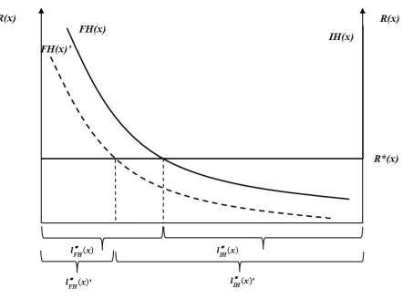
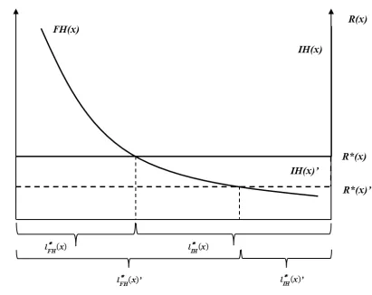
R x for a fixed level of R xH( ). This is illustrated by the FH x( ) curve in Figure 1. This curve

(27)

the horizontal axis represents the level of land rent. In the informal housing sector, each land developer maximizes the expected profits given by:

( )

max{ ( ) ( ) ( ) ( ) ( )} at each (0, ]

IH IH H IH IH IH f

l x



x 



R x A l x R x l x x x .

(1.13) The first order condition of (1.13) yields:

( ) ( ),

H IH

R x A R x



 (1.14)

which determines the demand for land in this sector. Since



and A_IH are taken as given by land developers, when



R x AH( ) IH R x( ) the informal land developer does not demand

land, and when



R x AH( ) IH R x( ) the demand does not exist. Finally, when

( ) ( )

H IH

R x A R x



 , any amount of land is demanded. This is illustrated by the IH x

 

curve in Figure 1. This curve is read from right-to-the left in the diagram. The free intersectoral land mobility establishes a common land rent in both sectors, which links them in a general equilibrium framework. In equilibrium, the land rent ensures that the value of marginal productivity of land is equal between sectors and that total land demand equals land supply. Thus, the equilibrium land allocation, at eachx, is characterized by:

* 1

( )

( )(1

)

[

/

(

)]

,

IH H H FH FH

A R x

R x

t

A

Z l

x





_

_





(1.15) which can be represented graphically as the intersection of the FH x( ) and IH x

 

curves in Figure 1. In this diagram the fixed land supply (which is equal to one) is represented by the length of the horizontal axis.12

(28)

[image:28.612.142.561.74.384.2]

Figure 1. Land market equilibrium at distance x to the CBD

In equilibrium, the land rent is then given by:

*

_{( )}

IH H

R

x





A R

x

, (1.16)

which is the value of the expected productivity in the informal housing sector.13_{Note from} (1.15) that it is always the case that:



(1

 

t

)



A

_FH

[

Z l

/

_FH*

( ]

x

)

1

A

_IH

,

which means that in equilibrium the marginal rate of transformation (right side of the equation) is equal to the relative price (for the producers) of the informal production in units of formal production (left side of the equation). Because both expressions depend of parameters that do not change with distance, it is clear that the equilibrium land allocation (as well the housing production)

13_{The rental rate of the public infrastructure}v x_{( )}_{is equal to the value of marginal productivity of public}

(29)

does not change with distance.14_{Using (1.15), it is possible to obtain the equilibrium land} allocation in the formal housing sector:

1/1 

*

[(1 ) / ]

FH FH IH

l Z t



A



A  , (1.17)

and the land allocation in the informal housing sector (recalling that the city is linear): 1/1 

*

1 [(1 ) / ]

IH FH IH

l  Z t



A



A  . (1.18)

Replacing (1.17) in (1.6), we find the housing production in the formal housing sector:

 /1 

* 1/

[(1 ) / ]

FH FH IH

Q Z t



A 



A   , (1.19) and replacing (1.18) in (1.7), we get the housing production in the informal housing sector:

1/1 

*

[(1 ) / ]

IH IH FH IH

Q A Z t



A



A  . (1.20) The total housing production at each distance x of the CBD is obtained adding the production of both sectors:

 /1 

* 1/

[(1 ) / ] [1 (1 ) / ]

IH FH IH

Q A Z t



A 



A    t

 

. (1.21)

Let Q*FH /l*FH 



AFH /





1t



be the building height in the formal housing sector and

* *

/

IH IH IH

Q

l



A

the building height in the informal housing sector. When (1.9) and (1.10) hold, it is possible to show that it is always the case that:



/ 1



t





1, implying that formal constructions are taller than informal constructions. Let q*_



A_FH /





1t



_l_FH* A_{IH IH}l* be the average tallness of the buildings. It is easy to verify that this expression is identical to total housing production. Then, Q* is also informative about the tallness of buildings. Assuming that formal and unemployed workers live close to the CBD, whereas informal workers live in

14_{If we had assumed a spatial variation in the infrastructure or in the probability of detection (or in any other}

(30)

the periphery (an equilibrium result that we will show below), the population constraints are given by: * * 0 d I x N

Q d

x

 

N L



, (1.22)

and * * * f d I x N x

Q dx L



. (1.23)

By rearranging (1.22) and using (1.21), it is possible to find the frontier between the formal workers zone and the informal workers zone:

* * I d N

N L

x

Q





, (1.24)

whereas by rearranging (1.23) and using (1.22) and (1.21), it is possible to find the city fringe: * * f

N

x

Q



. (1.25)

Note that the city fringe x*_f , through the housing production, depends of taxes, infrastructure, the probability of detection, total factor productivity in the formal housing sector, and land productivity in the informal housing sector. Also note that the land allocation, the housing production, and the city fringe x*_f do not depend on the utility levels. This is a consequence of the assumptions of fixed housing consumption and perfect substitutability between the formal and the informal production. Now we can find the equilibrium values of the instantaneous utilities

W

_F*

,

W

_U*

,

W

_IN* and the equilibrium housing rent

R x

_H*

( )

. The corresponding bid rents for each worker type are given by the following equations:

( , )

F x WF wF



x WF

    , (1.26)

( , )

IN x WIN wIN sIN



x WIN

    , (1.27)

( , )

U xWU wU



x WU

(31)

[image:31.612.91.553.183.496.2]

These functions are linear and decreasing in x. The bid rent for a formal worker and the bid rent for an unemployed worker share the same level of inclination. Also both bid rents are steeper than the bid rent for an informal worker. Then, in equilibrium, formal workers and the unemployed live close to the CBD, whereas informal workers live in the periphery (Figure 2).

Figure 2. Urban land use equilibrium (The segregated city)

(32)

* *

F U F U

W



W



w



w

, (1.29)

* *

IN IN

U U IN IN IN

N L

w

W

w

s

W

Q



















_

_







_

_











, (1.30)

*

0

IN IN IN

N

w

s

Q

W









, (1.31)





* * * * *

( ) max ( , ), ( , ), ( , ),0 for each (0, ]

H F F U U IN IN f

R x   x W  x W  x W x x .

(1.32)

Equation (1.29) implies that the bid rent for a formal worker is equal to the bid rent for an unemployed all over the city. Equation (1.30) implies that exactly at the frontier between the formal workers zone and the informal workers zone,

x

*_d, the bid rent for a formal worker is equal to the bid rent for an informal worker. Equation(1.31), in turn, means that exactly at the city fringe the bid rent for an informal worker is equal to the agricultural rent (which is assumed to be zero). Equation(1.31), together with (1.16), guarantees that the equilibrium land rent is equal to agricultural rent at the city fringe. Finally, Equation (1.32) states that the equilibrium housing rent is equal to the upper envelope of the equilibrium bid rent curves of all workers and the agricultural rent line (Zenou, 2011). The equilibrium values of the instantaneous utilities for the formal, unemployed and informal workers can be obtained by using equations (1.29) to (1.31):

*

IN IN IN

W

w

s

N

Q







, (1.33)

*

(1

)

*

IN

U U IN

L

N

W

w

s

Q







 

, (1.34)

*

(1

)

*

IN

F F IN

L

N

W

w

s

Q







 

. (1.35)

(33)

* * * *

* * *

*

(1

)

for

0 ,

for

,

0 fo

(

.

)

r

IN IN IN IN H IN

L

N L

N

x

s

x

Q

N L

N

R

s

x

Q

x

N

x



 

_



_{ }

_{ }



 









_

_

_





_

_



_

 













(1.36) Note that (1.36) together with (1.16) implies that the equilibrium land rent is described by:

* * *

*

* * *

*

(1 ) for 0 ,

for ,

0 for .

( )

IN IN

IH IN

IN

IH IN

L N L

N

A x s x

Q Q Q

N L

N N

R A s x x

Q Q Q

N x Q x











                          _ _ _  _ _  _            (1.37)

Finally, defining the urban cost for a worker as the sum of the housing rent and the commuting cost, we have that in equilibrium, the urban cost for a formal worker is

* *

(N Q ) (1 sIN) (LIN Q )



 



, and for an informal worker it would be sIN



(N Q*).

1.4. Urban labor market equilibrium

1.4.1. Lifetime expected utility for workers and firms

Workers discount future values at a rate

r

. Let I_F, I_U, and I_IN denote the expected lifetime utility for a formal worker, for an unemployed worker and for an informal worker, respectively. In the steady-state, the Bellman equations for I_Fand I_IN are given by:









*

1

*

IN

F F IN F F U

L

N

rI

w

s

I

Q









 



, (1.38)





*

IN IN IN IN U IN

N

rI

w

s

I

Q





(34)

which show that workers obtain their instantaneous utility in each period. Furthermore, formal workers can lose their jobs at a rate



_F, which leads to a surplus loss of I_F I_U. Informal workers, in turn, can lose their jobs at a rate



_IN, so their change in surplus is given by I_U I_IN. In the steady-state, the Bellman equation for I_U is given by:





 







*

1

*

IN

U U IN F U IN U

L

N

rI

w

s

q

I

b I

Q



 







 







 

.

(1.40)

This equation shows that, besides obtaining her instantaneous utility, an unemployed worker can obtain either a job in the formal sector at a rate

 

q( ) (since s_U 1 ), with an accompanying increase in surplus of I_F I_U, or a job in the informal sector at a rate



, with a surplus change of I_IN  b I_U (recall that

b

is the present value of the sum of all the transfers received while informally employed). Given that there are no relocation costs, in equilibrium all workers must reach the same utility level independently of their location in the city, therefore:

I

_F



I

_F,

I

_U



I

_U and

I

_IN



I

_IN. Using (1.39) and (1.40) we obtain:





*

 



1

1 IN

U IN U IN IN F U

IN

N L

I I w w s b q I I

r

 



Q



 

    

  _    _ _   _

  _ _ _ _,

(1.41)

whereas by using (1.38) and (1.40) we get:

 





1

F U F U U IN

F

I I w w b I I

r



 

q



  _     _

  . (1.42)

Then, replacing (1.41) in (1.42) we obtain:

 





1 

_* IN







1 

F U IN F IN IN IN U

N L

I

r

w

s

r

b

w

(35)

where

 

 

1 



r



F



r 

 

IN





 

q

 

r



IN



 and

 





r 

 

IN



.

Denoting the search cost per unit of time for a formal firms as c, we have that the value of a vacancy I_V and a filled vacancy I_Oare given by:

 



V O V

rI   c q



I I , (1.44)





O F F F O V

rI  y w  T



I I . (1.45)

Firms are free to post vacancies and they do until I_V 0. This, together with (1.44) implies that:

( )

O

c

I

q





. (1.46)

If we useIV 0, and equations (1.45) and (1.46), we have the following equation

determining job creation in the formal sector:

 

F FF

y w T

c

q



r



 

 

. (1.47)

1.4.2. Wages in equilibrium

At each period, wages are set through a generalized Nash-bargaining process between firms and workers:



 



1

argmax

F

F F U O V

w



I



I



I



I

, (1.48)

where 0 



1 represents the bargaining power of workers. By solving (1.48) we obtain:



1 



1 

*







1 



1 

IN

F IN IN IN U F

N L

w

s

r

b

w

y

T

c

Q

 



























 

 

_

_

 

_

_

 

_

 

_





_

  



_

















(36)

The first term in (1.49) is the compensation that firms must pay to induce workers to accept a job in the formal sector. The compensation is the fraction



1





of the expected income obtained by the worker outside the formal sector, which is a weighted average of the unemployed current income w_U and the informal worker income,



 





*







1

IN IN IN IN

w

 

s



N L



Q

 

r



b

, being



1





and



the respective weights. This compensation is different from the one obtained in urban labor models without an informal sector or with a residual informal sector (Wasmer and Zenou, 2002; Zenou, 2008; and Zenou, 2011), where firms only compensate the unemployed worker with a fraction of his current income. This is because, in contrast with the mentioned models, here firms acknowledge that an unemployed worker can find a job in an informal sector that offers intrinsic benefits. One of these benefits is the urban cost saving for the informal worker, given by the difference between the urban cost for a formal worker and the urban cost for an informal worker:



1 

s

_IN

 





N L



_IN



Q

*



. This difference is always positive, reflecting the fact that an informal worker commutes less often to the CBD.

(37)

1.4.3. Informality and unemployment rates, and the steady-state equilibrium

The structure of the model allows for deriving explicit analytical expressions for the informality rate and the unemployment rate. In the steady-state, two conditions must hold: first, that the number of unemployed workers that find a formal job,

 

q

 

U, equals the number of workers that lose their formal jobs,



_FL_F, and second, that the number of unemployed workers that find an informal job,



U

, equals the number of informal workers that lose their job,



_INL_IN. Therefore, given thatU  N L_FL_IN, the following must hold:

 



FLF q N LF LIN





 

  , (1.50)





INLIN N LF LIN







  , (1.51)

which implies that the informality rate



* and unemployment rate u* in the steady-state are given by:





 

* F

F IN IN q

 



 



  



  , (1.52)





 

* F IN

F IN IN

u

q

 



  



  . (1.53)

It is possible to verify that (



*  



) 0,

(



u

*

 



)

0

, which shows that an increase in formal job creation leads to a decrease in both the informality and the unemployment rates. Given a certain value of the labor market tightness



, it is possible to determine all the endogenous variables in the model. Replacing (1.49) (the equilibrium wage in the formal sector) and (1.52) (the informality rate in the steady-state) into (1.47), we obtain the following condition determining the formal job creation rate in equilibrium



*:





_{ }

























* * * *

1

0.

F

F IN IN IN U

c

r

c

q

N

y

w

s

r

b

w

(38)

Let  be the expression on the left hand side of (1.54). Assuming that formal sector productivity is always higher than the expected income of the unemployed, i.e. assuming that:



1 

IN _*







1 

F IN IN IN U

IN

N

y

w

s

r

b

w

T

Q

























_

 

_

_

 

_

 













,

(1.55)

it is always the case that

0

( ) 0, lim , lim 0

 



 

        . Thus, there must be a unique

*



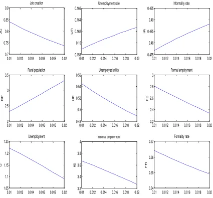
that satisfies equation (1.54), and consequently, there is a unique steady-state equilibrium.

1.5. Comparative statics

In this section, we investigate the effects of changes in the city's parameters over the job creation rate



*, the informality rate



*_{, the housing rent} *

 

H

R x and the land rent R x*

 

. We pay special attention on the parameters that give shape to the structure of the city: 1) the level of centralization of the informal sectors_IN in the labor market 2) the commuting cost per unit of distance



, 3) the provision of the public infrastructure

Z

, 4) the added value taxes t charged to formal land developers , and 5) the probability of detection of an informal land developer



(see the Appendix A for formal proofs).

1.5.1. Decrease in the informal sector centralization

Recall that a decrease in the commuting frequency of an informal worker is always followed by an increase of the wage fraction generated through home-based work. Spatially, this can be seen as a decrease in the informal production at the center and a rise of the informal production in the periphery. As a consequence, the effects on the economy of a decrease in

IN

s provide an idea of the effects on the economy of a lower degree of centralization of the informal sector.

Informality in the City: a Theoretical Analysis