OPTIMIZING CALCULATIONS OF EDGE DIFFRACTION IMPULSE
RESPONSES FOR ROOM ACOUSTICS COMPUTATIONS
PACS: 43.55.Ka
Torres, Rendell R.(1); Svensson, U. Peter(2)
(1) Program in Architectural Acoustics Rensselaer Polytechnic Institute (RPI) 110 8th St., Greene Bldg.
Troy, NY 12180-3590 USA Tel: +1-518-276 6925 Fax: +1-518-276 3034 E-mail: rrtorres@rpi.edu
(2) Acoustics Group, Department of Telecommunications Norwegian University of Science and Technology (NTNU) NO-7491 Trondheim NORWAY
Tel: +47-73 59 05 46 Fax: +47-73 59 14 12
E-mail: svensson@tele.ntnu.no
ABSTRACT
Measurements of edge diffraction from panels have shown interesting implications for room acoustics computation [1]. Further analysis is possible using numerical studies such as Svensson’s extension of the Biot-Tolstoy-Medwin (BTM) method [2]. This approach allows one to include higher orders of edge-diffraction, although each additional order increases computation time. Studies of diffraction order are done to determine when inclusion of higher orders is necessary or may be neglected for applications such as interactive auralization.
INTRODUCTION
In order to minimize the computational demands of including scattering in auralization, it is appropriate to study how many orders of scattering need to be included. For this purpose, studying edge diffraction is especially appropriate, since edge diffraction can be considered an elementary form of surface scattering. In a previous study incorporating edge-diffraction computations and initial listening tests [3], it was found that higher orders and combinations of edge diffraction components were not usually as significant as first-order diffraction components. Additionally, the total diffraction effects within the audible frequency range were relatively small above about 150 Hz. The reason for this was that the reference geometry (a large concert-hall stagehouse) was conservatively composed of large flat walls whose dimensions were larger than most of the wavelengths of interest. This was “conservative” in the sense that only the longest wavelengths of interest would give rise to significant edge-diffractions, and the study investigated whether in such cases the diffraction was audible in listening tests. The results interestingly showed that these diffraction effects were still audible for various input signals.
SINGLE PANEL DIFFRACTION
To most clearly illustrate the effect of calculating varying orders of diffraction, we initially consider only one reflector. Figure 1 shows on the left an elevation of the source-panel-receiver configuration. The rectangular reflector under study in this computational investigation corresponds to retaining only reflector “L3” from the array shown in plan on the right.
R1 R7 R13
50 80 110
[image:2.596.87.516.176.321.2]x [cm]
(50)
(110)
50
cm
L1 L5 L2 L4 L3 C.L. 85 cmFIGURE 1. Orientation of source, panel reflector, and receiver R7.
The panel is 12 cm wide and 105 cm long. The omnidirectional source is represented by the solid black circle, and the receiver is at 80 cm from the source (receiver R7) in the computations below, unless noted otherwise. Tick marks on the x-axis represent 5-cm increments. The dashed line represents a wavefront’s direction. The dotted lines represent the geometrical-acoustics reflection zone (or “specular zone”) for the center reflector L3. The receiver is depicted here at 80 cm (offset from the centerline by 3 cm), such that the reflection point is essentially at the center of the array (but offset from the centerline by 1.5 cm). The triangular “arrowheads” above the reflector arrays point to the specular-reflection points corresponding to the microphone positions on the lower scale. (The numbers in parentheses and the arrowhead-spacing are not in centimeter units.)
TIME-DOMAIN EDGE-DIFFRACTION COMPUTATIONS
The edge-diffraction model is discussed and benchmarked in Refs. [2,3]. In Svensson’s extension of the Biot-Tolstoy-Medwin (BTM) approach [4], the edges are divided into sources with analytically derived strengths [2]. One sample of the edge-diffraction impulse response h is given by the following (Eq. 35, [2]):
(
)
z
ml
h
S Ri
≈
−
∆
∆
,
,
,
,
4
θ
θ
γ
α
β
π
ν
(1)where
∆
z
is the length of the source at zi along the edge,ν
describes the wedge angle, m and l are source and receiver distances, and β is an analytical edge-source directivity-function that depends on the angles corresponding to the source and receiver orientations relative to a given edge.RESULTS
FIGURE 2. In the left figure the total impulse response is computed for the rectangular reflector L3. The specular and diffractive components are computed as separate impulse responses, as magnified in the right figure.
Note that the edge diffraction combines with the specular (image) reflection to yield the total scattering from the reflector panel. One of the advantages of a time-domain model is that one can clearly link edges’ contributions to different orders of diffraction and, consequently, to the sound field at different frequencies. Another advantage of the time domain formulation is that it is suitable for complementing commonly used room acoustics programs based on geometrical acoustics. Moreover, one can calculate the diffraction impulse responses directly (instead of transforming from the frequency domain computations) and then add them to the geometric components to obtain the total field.
Comparisons of First- and Second-Order Diffraction
Figures 3-5 illustrate and compare the effects of including first- and second-order diffraction in computations.
[image:3.596.177.410.520.715.2]Low-frequency fall-off The solid line in Figure 3 corresponds to inclusion of up to second-order diffraction and shows the expected fall-off in scattered energy at lower frequencies due to diffraction “around” the panel (such that less energy is reflected specularly toward the receiver). The dashed curve corresponds to including only up to first-order diffraction and deviates from the expected fall-off as the frequency decreases. Without including higher orders of diffraction, the total computed response at lower frequencies becomes increasingly incorrect.
Relative levels of diffraction orders It is easier to understand the previous results by examining the relative levels of each diffraction order as a function of the ratio between the panel width d and the wavelength, λ. In Figure 4, first-order diffraction becomes significant when the wavelength is approximately on the order of the panel width. (The precise “intersection” point can vary with the angles of the source and receiver to the edges.) For this receiver position, the first-order diffraction has opposite sign compared to the specular reflection, and the resulting cancellation effect becomes stronger with decreasing frequency, resulting in the fall-off observed above. However, higher-order diffraction is also necessary for this fall-off to continue with decreasing frequency/longer wavelength. This is evident in the fact that second-order diffraction rises more steeply with increasing wavelength and thus has greater “corrective” effect at lower frequencies.
FIGURE 4. Relative levels of edge diffraction to specular reflection, plotted with respect to the ratio of width to wavelength (or kd/2π, where k is wavenumber). The level of the specular reflection is shown at 0 dB. The significance of edge diffraction is clear for longer wavelengths.
“Error” from neglecting second-order diffraction Figure 5 shows the difference (as a function of the ratio of width d to wavelength) in the computed scattered energy with second-order diffraction to that with only first-second-order, where the difference is computed as a ratio between the two cases. The inclusion of second-order diffraction begins to be apparent when the wavelength becomes longer than the width of the panel, and becomes significant when the wavelength exceeds approximately twice the width. Moreover, this may also be seen as a way to express the “error” that results when second-order diffraction is neglected. For example, for a finite panel whose characteristic dimension corresponds to the wavelength at 2900 Hz (as for this 12-cm panel width), the error in this case would be as large as 6 dB at 290 Hz and further increase with lower frequencies. Such errors become even more significant when several reflecting surfaces in a room (such as architecturally articulated walls) are composed of irregularities of similar scale.
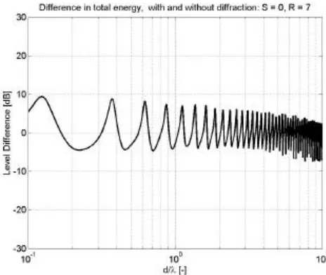
Difference in Total Energy
responses at longer wavelengths relative to the scatterer size (or dimension of surface irregularity).
FIGURE 5. Level difference in computed scattered energy from reflector panel when up to second-order edge diffraction is included.
FIGURE 6. Level difference in total energy (including direct sound) when up to second-order edge diffraction is included.
CONCLUSIONS AND CURRENT WORK
[image:5.596.176.410.119.315.2] [image:5.596.177.409.380.576.2]receiver orientations for different elementary geometries in order to determine reliable guidelines for such computational partitioning.
BIBLIOGRAPHICAL REFERENCES
[1] R. R. Torres et al., “Studies of Scattering from Faceted Room Surfaces,” Proc. of Intl. Congress on Acoustics (ICA), Rome (2001)
[2] U.P. Svensson et. al, “An analytic secondary source model of edge diffraction impulse responses,”J. Acoust. Soc. Am. 106, 2331–2344 (1999)
[3] R. R. Torres et al., “Computation of edge diffraction for more accurate room acoustics auralization,” J. Acoust. Soc. Am. 109, 600–610 (2001)
[4] H. Medwin, “Shadowing by finite noise barriers,” J. Acoust. Soc. Am. 69, 1060-1064 (1981)