TAKING INTO ACCOUNT THE TEMPORARY AND SPECTRAL
STRUCTURE OF THE SOUND ENERGY FOR THE
CHARACTERIZATION OF THE ANNOYANCE GENERATED BY THE
ROAD AND RAILWAY TRAFFIC
Antonio J. Torija1, Diego P. Ruiz1, Dick Botteldooren2, Bert De Coensel2
1 Departamento de Física Aplicada, Universidad de Granada, Avda. Fuentenueva s/n, 18071 Granada, España.
2 Acoustics Group, Department of Information Technology, Ghent University, St. Pietersnieuwstraat 41, B-9000
Ghent, Belgium.
E-mail: ajtorija@ugr.es; druiz@ugr.es; dick.botteldooren@intec.ugent.be; bert.decoensel@intec.ugent.be
Resumen
Tal y como han indicado numerosos autores, los sistemas de transporte masivo representan una de la mayores externalidades ambientales. Los grandes ejes viarios y ferroviarios generan un elevado grado de disconformidad en la población adyacente, debido entre otras cosas, a la gran contaminación sonora generada. Dicha contaminación sonora junto al nivel emitido, posee una serie de características temporales y espectrales, que obliga a considerar más factores junto al descriptor LAeq, para evaluar el impacto sobre la población afectada. A su vez, debido a que las características de circulación del tráfico rodado y del tráfico ferroviario son totalmente diferentes, conviene estudiar por separado dichas situaciones y caracterizar el impacto sonoro generado. Por ello, en este trabajo vamos a llevar a cabo un análisis de la estructura temporal, en cuanto al nivel de variabilidad de la energía sonora recibida, el factor cresta de la señal, etc. y de la estructura espectral, con factores como presencia de componentes tonales, variabilidad espectral de la energía sonora, porcentaje de energía sonora en frecuencias críticas, etc., como complemento al nivel de energía sonora emitido para la evaluación del impacto sonoro generado por los grandes ejes viarios y ferroviarios sobre la población expuesta.
Palabras-clave: Ruido, Tráfico rodado, Tráfico ferroviario, Molestia percivida.
Abstract
As several authors have indicated, the massive transport systems represent one of the most important environmental externalities. The big road and railway axis generate a high degree of annoyance in the adjacent population, due, among other things, to the large amount of generated sound pollution. The above mentioned sound pollution possesses a series of temporary and spectral characteristics, as well as of emitted energy level, which forces us to consider more factors besides of the LAeq descriptor, to evaluate the impact on the affected population. In turn, due to the fact that the circulation characteristics of the road and railway traffic are totally different, it suits to study separately the above mentioned situations and characterize the generated sound impact. For it, in this work we carried out an analysis of both the temporary structure, (the variability level of the received sound energy, the crest factor of the sign, etc), and the spectral structure, through factors such as tonal components, spectral variability of the sound energy, percentage of sound energy in critical frequencies, etc. The proposed factors are to be seen as a complement to the average level of exposure level of the sound energy for the evaluation of the sound impact generated by big roads and railway axis on the exposed population.
2
1
Introduction
The environmental externalities generated by the transportation systems, both big road and railway traffic axis, represent one of the most important threat for the well-being of the exposed population [1, 2]. More generally, the demand of urban and interurban mobility should be relieved with the development of an inhabitable and agreeable soundscape and, therefore, to obtain a minimization of its negative impact on the man and on the environment. For the achievement of a suitable sound environment for the population, one of the most important parameters to considering is the generated annoyance level [3].
In fact, of the environmental pollution factors that are affected by the use of transportation means, noise is perhaps the most commonly cited [4]. Besides, the different means of transport in traffic (road and railway traffic) have very diverse characteristics, generating different sound pressure levels, with a different spectral composition, appearance of pure tones, with a certain temporary structure, more or less impulsively, etc., which can originate differences in the generated annoyance levels.
There are several studies about this topic [5-8], studying the annoyance levels generated by the road and railway traffic on the exposed population, obtaining different conclusions according to the author as for the difference in perceived annoyance between train and road traffic noise at the same average sound level. Now, with the introduction of high-speed trains and train-like transportation systems based on magnetic levitation (maglev), the question has arisen whether a difference in perceived annoyance of trains and highway noise still exits [9].
In addition, many authors [10-13] establish the need to have parameters that allow us to characterize and to describe the annoyance produced by the road and railway traffic, since the utilization of the parameter LAeq, it does not seem to be sufficiently precise, due to the large amount of factors that influence the generation of annoyance and, that are not included by this parameter [14, 15]. The European [16] and national [17] authorities establish limits of sound quality for the road and railway traffic axis based on LAeq values, so that, due to the multiple deficiencies presented by this descriptor, the accomplishment of these limits does not seem to satisfy the affected population, since is not considered to be the temporary and spectral structure of the sound energy an element of diagnosis for the characterization of the environment as more or less pollutant.
Therefore, in this work the main goal is the analysis of the temporary and spectral structure, together with the overall level, of the sound energy generated by the traffic as element of characterization of the level of annoyance generated by the road and railway traffic, so that we could construct a model what, based on the characteristics of the sound energy that affects on the exposed population, is able to predict the generated annoyance level. For it we are going to use a series of factors, which allow us to describe so much the temporary as spectral structure, so that we are going to approach the behavior of each one of these factors with regard to the level of annoyance.
2
Methodology
2.1 Temporary structure of the sound energy
3
and railway traffic, in the environments affected by these means of transport, we find a certain level of sound energy, which have a certain temporary structure. The appearance of fluctuations of sound energy are typical of this type of sound environments as well as the appearance of big increases of sound energy generated by the circulation of road and railway traffic.
In this research, we focus on the analysis of the temporary macrostructure of the generated sound environment, like element of diagnosis of the generated annoyance level. Some studios [18] establish the great relationship between the supra-second structure and the annoyance level generated by the traffic noise. For the characterization of the temporary macrostructure of the sound energy generated by the road and railway traffic we are going to use the following factors, the Temporal Sound Energy Deviation (TSED) and the Crest Factor (CF) of the signal.
In this work the temporal sound energy deviation is defined like the level of temporal variability of the sound energy of a certain location, resultant of the combination of the variability of the instant sound energy level and the variability of the accumulated sound energy level for a certain time interval [19].
(1)
where:
TSED = Temporal sound energy deviation.
ISE = Instant sound energy variability.
ASE = Accumulated sound energy variability.
The utilization of this parameter allows the characterization of the temporary evolution of the sound energy, so that the appearance of big increases of energy is going to be represented by increases in the value of the parameter TSED. The sound environments affected by road and railway traffic are exposed to big fluctuations in the sound energy levels, fluctuations that cause increases and decreases in the amount of sound energy received by the receptor. But, in addition, the fluctuations, above the average value of sound energy, generate the appearance of different values of incident sound energy, for what the analysis of the variability of the accumulated sound energy for the characterization of the evolution of the received energetic level is very interesting, since great increases in the instant sound energy generate high values in the instant sound energy variability and in the accumulated sound energy variability and, therefore, we obtain a high TSED value. However, when the values of instant sound energy variability are very high but the input of sound energy in the environment is very low, the accumulated sound energy variability value is close to 0 and, therefore, the value of TSED is lower.
On the other hand, the crest factor is defined like the existing relation between the extent of the waveform peak amplitude and its RMS value. The importance of the calculation of this parameter is to know the impulsiveness degree that presents the sound energy level in a certain time interval.
(2)
4
2.2 Spectral structure of the sound energy
The frequency composition of the noise is also important in the matter of characterize the sound environment. The soundscapes affected by the road and railway traffic has a large composition in low frequencies, especially at about 60 Hz. This spectral composition generates the appearance of auditory and non-auditory effects, described not only for the A-weigh applied at the sound pressure level.
Therefore, the only utilization of the parameter LAeq for the characterization of the annoyance generated by the road and railway traffic does not seem to be very suitable, since as Berglund et al. [20] establishes LAeq may be a good metric for assessing the risk for hearing impairment, however it may be less well suited for estimating (perceived) annoyance evoked by sounds with a large portion of low-frequency components.
For this reason, in this work we have realized an analysis to know which are the critical bands of frequency for the description of the annoyance level generated by the road and railway traffic. For it, we have studied the influence that has the value of the percentage of sound energy in these critical bands of frequency, for the characterization of the annoyance level generated on the population. The importance of this analysis is in contracts the A-weigh with the range of critical frequencies, with a greater correlation level with the perceived annoyance, to verify its proximity, and to be able to estimate the deficiency degree of this A-weigh for the description of the perceived annoyance generated by the road and railway traffic.
Other of the aspects related to the spectral structure of the sound energy with a great impact in the perceived annoyance level is the appearance of pure tones (or tonal components) [21]. Several studies indicate that tonal components should be taken into account when the likelihood of noise annoyance is assessed [22]. No agreement has been reached concerning the size of the penalty to be added to the sound level when the noise contains tone. One problem is that the effect of a tone seems to depend on the frequency of the tone, its, level, the total spectral character and level of noise [23]. According to Hellman [24], noise annoyance may also be influenced by the number of tones in the noise spectrum. Therefore, in this research, we have realized an analysis of the number of tonal components in the spectrum of each one of the studied stimuli, as well as an analysis of the influence of its position inside the spectrum at the time of studying its relation with the perceived annoyance level.
On the other hand, other of the factors used for the characterization of the spectral structure of the sound energy has been the distribution of the sound energy in the noise spectrum. The analysis of the distribution of the sound energy along the spectrum has been estimated by means of the utilization of the parameter Spectral Sound Energy Deviation (SSED).
(3)
Where
SSE = Variability of the sound energy in the noise spectrum.
5
2.3 The experiment
The accomplishment of the experiment [9] is based on a sound reproduction in a realistic setting; the goal was to obtain an “ecologically valid” reproduction. For it, during the experiment, subgroups of participants were seated in the living room, reading a magazine, engaging in light conversation or having something to drink. Traffic sounds were reproduced for two loudspeakers placed outdoors. The procedure consisted of 2 phases. Firstly, the sound was recorded outdoor by 2 B&K 4189 free field microphones separated 20 m from each other along the track; for calibration, the façade level was also recorded. At the same time, a binaural recording was made inside the house. Secondly, the recorded sound was played back by 2 loudspeakers in front of the house, separated about 10 m from each other, and along the same horizontal axis as seen from the window. The volume was adjusted to reproduce the 1/3-octave band spectrum at the façade as accurately as possible. Simultaneously, a binaural recording was again made inside the house. Ideally both binaural recordings (real and reproduced) should be equal. The binaural recording inside the house was made by means of an artificial head.
Two-channel recordings were conducted for three types of trains. Two microphones were placed at 20 m distance from each other along the track, 2.5 m above ground level. The recorded trains were TGV trains at high speed (approx. 140 Km/h and 300 Km/h), Dutch intercity (IC) trains of the new type (duplex) (approx. 140 Km/h) and Maglev trains (Transrapid 08 train) at high speed (approx. 200 Km/h, 300 Km/h and 400 Km/h). The recordings were realized at different distances (25 m, 50 m, 100 m and 200m).
The panelists were exposed to experimental sound during 10 minutes (henceforth called menu). Menus with 2 or 4 passages were created, with the random appearance of the same train type, at the same distance and speed.
On the other hand, the sound of the E40 highway was also recorded near Ghent (Belgium), a 10-minute highway sound was recorded at 50 m distance to the closest lane. Besides, highway sound was recorded at different distances 10 m, 15 m and 100 m.
To guarantee a representative sample of panelists was realized a selection of 100 panelists on the basis of fuzzy resemblance to the typical Dutch person on the most critical criteria of annoyance surveys.
Four to six panelists jointly participated in a session. The overall structure of the experiment was identical for each group of panelists. It started with a 14-minute training session, thereafter, 7 10-minute menus were played, of which the first menu always was the highway traffic menu. A short break was then taken and the training session was repeated, after which again 7 new 10-minute menus were played. In all, two time 6 train menus were presented to each panelist.
6
3
Results
3.1 Critical frequency bands and tonal components
[image:6.595.66.534.348.741.2]When we analyze the impact of the sound energy in each of the 1/3-octave bands on the perceived annoyance level (table 1) we verify, obviously, a more or less high value depending on the 1/3-octave band that we consider. We can observe that the sound energy accumulated in the low frequencies has a high degree of correlation with the perceived annoyance level. Due to this, we can conclude that the utilization of the A-weigh for the characterization of the annoyance generated by the road and railway traffic is not very suitable, since this A-weigh attenuates the low frequencies, which impedes that are included non-auditory with a great impact in the level of disturbance, effects related to the presence of noises by a large amount of energy in the low frequencies [15]. Therefore, in view of the results showed in the table, we can establish a range of critical 1/3-octave bands for the description of the annoyance generated by the road and railway traffic on the exposed population. These critical bands are included in the interval 31.50-125 Hz, 315 Hz and 630-2500 Hz.
Table 1. Analysis of the relationship between the sound energy in each of the 1/3-octave bands and the master scaling units. The bilateral significance is shown at the bottom. *p<0.05, **p<0.01
1/3-octave band
Pearson Correlation (r) Kendall Correlation (Tau b) Spearman Correlation (Rho)
Coefficient Bilateral
sig. Coefficient Bilateral sig. Coefficient Bilateral sig.
20 Hz 0.083 (*) 0.022 0.096 (*) 0.017 0.141 (*) 0.019
25 Hz 0.071 (*) 0.027 0.098 (*) 0.015 0.151 (*) 0.012
31.50 Hz 0.424 (**) 0.000 0.262 (**) 0.000 0.369 (**) 0.000
40 Hz 0.547 (**) 0.000 0.358 (**) 0.000 0.505 (**) 0.000
50 Hz 0.411 (**) 0.000 0.240 (**) 0.000 0.350 (**) 0.000
63 Hz 0.586 (**) 0.000 0.402 (**) 0.000 0.568 (**) 0.000
80 Hz 0.530 (**) 0.000 0.356 (**) 0.000 0.510 (**) 0.000
100 Hz 0.406 (**) 0.000 0.284 (**) 0.000 0.410 (**) 0.000
125 Hz 0.227 (**) 0.000 0.163 (**) 0.000 0.234 (**) 0.000
160 Hz 0.159 (**) 0.000 0.098 (*) 0.016 0.147 (*) 0.015
200 Hz 0.114 0.059 0.080 (*) 0.048 0.115 0.057
250 Hz 0.137 (*) 0.023 0.093 (*) 0.022 0.138 (*) 0.022
315 Hz 0.186 (**) 0.002 0.122 (**) 0.003 0.178 (**) 0.003
400 Hz 0.102 0.092 0.081 (*) 0.046 0.115 0.058
500 Hz 0.052 0.389 0.036 0.369 0.055 0.366
630 Hz 0.173 (**) 0.004 0.124 (**) 0.002 0.183 (**) 0.002
800 Hz 0.426 (**) 0.000 0.293 (**) 0.000 0.422 (**) 0.000
1000 Hz 0.522 (**) 0.000 0.362 (**) 0.000 0.514 (**) 0.000
1250 Hz 0.404 (**) 0.000 0.275 (**) 0.000 0.393 (**) 0.000
1600 Hz 0.183 (**) 0.002 0.137 (**) 0.001 0.190 (**) 0.002
2000 Hz 0.295 (**) 0.000 0.191 (**) 0.000 0.273 (**) 0.000
2500 Hz 0.211 (**) 0.000 0.145 (**) 0.000 0.203 (**) 0.001
3150 Hz 0.002 0.978 0.017 0.669 0.020 0.735
4000 Hz -0.036 0.556 -0.012 0.767 -0.018 0.770
5000 Hz -0.041 0.500 -0.030 0.455 -0.047 0.441
6300 Hz -0.028 0.642 -0.006 0.875 -0.012 0.846
8000 Hz -0.071 0.242 -0.032 0.430 -0.045 0.456
10000 Hz -0.071 0.241 -0.028 0.490 -0.044 0.469
12500 Hz -0.065 0.280 -0.030 0.451 -0.045 0.457
16000 Hz -0.080 0.186 -0.047 0.246 -0.069 0.257
7
Due to this, the accumulation of sound energy in these 1/3-octave bands is going to cause the appearance of high values in the perceived annoyance level.
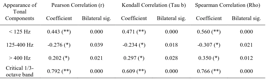
[image:7.595.67.531.254.392.2]On the other hand, when we analyze the impact of the appearance of tonal components on the perceived annoyance level (table 2), we verify that the position of the tonal component has great influence in the generated effect.
Table 2. Relationship between the appearance of tonal components (pure tone) in the different frequency ranges and the master scaling units. The bilateral significance is shown at the bottom.
*p<0.05, **p<0.01
Appearance of Tonal Components
Pearson Correlation (r) Kendall Correlation (Tau b) Spearman Correlation (Rho)
Coefficient Bilateral sig. Coefficient Bilateral sig. Coefficient Bilateral sig.
< 125 Hz 0.443 (**) 0.000 0.471 (**) 0.000 0.560 (**) 0.000
125-400 Hz -0.276 (*) 0.039 -0.234 (*) 0.018 -0.307 (*) 0.021
> 400 Hz 0.202 (*) 0.021 0.297 (*) 0.028 0.350 (*) 0.012
Critical
1/3-octave band 0.792 (**) 0.000 0.609 (**) 0.000 0.766 (**) 0.000
Analyzing the complete range of frequencies we verify as the tonal components of low frequencies has a high impact on the generated annoyance level, being higher than the impact of the tonal components of medium-high frequencies. Studying the relation of the tonal components, placed in the critical 1/3-octave bands, on the perceived annoyance level we observe a high level of correlation (Pearson coefficient r = 0.792).
3.2 Temporary and spectral structure for the estimation of the perceived annoyance
Observing the results showed in the table 3, we verify that parameters habitually used for the characterization of the perceived annoyance, LAeq (Pearson coefficient r = 0.559) and Zwicker Loudness (Pearson coefficient r = 0.390), do not have a high value of correlation with the annoyance level generated by the road and railway traffic. We can observe that the correlation level of these factors is even smaller than the correlation level between the perceived annoyance and the received sound energy level without weigh, Leq (Pearson coefficient r = 0.770).
8
[image:8.595.65.532.187.419.2]coefficient r = 0.841) have therefore, a great impact in the perception of annoyance generated by road and railway traffic.
Table 3. Relationship between LAeq, Zwicker Loudness, Leq and temporary and spectral structure factors with the perceived annoyance level. The bilateral significance is shown at the bottom. *p<0.05,
**p<0.01
Factors
Pearson Correlation (r) Kendall Correlation (Tau b) Spearman Correlation (Rho)
Coefficient Bilateral sig. Coefficient Bilateral sig. Coefficient Bilateral sig.
LAeq 0.559 (**) 0.002 0.419 (**) 0.000 0.480 (**) 0.000
Zwicker
Loudness 0.390 (**) 0.003 0.240 (**) 0.009 0.348 (**) 0.000
Leq 0.770 (**) 0.000 0.521 (**) 0.000 0.699 (**) 0.000
TSED 0.614 (**) 0.000 0.514 (**) 0.000 0.520 (**) 0.000
CF 0.570 (**) 0.000 0.425 (**) 0.000 0.447 (**) 0.000
PSE 0.885 (**) 0.000 0.697 (**) 0.000 0.860 (**) 0.000
TCA 0.792 (**) 0.000 0.609 (**) 0.000 0.766 (**) 0.000
SSED 0.841 (**) 0.000 0.588 (**) 0.000 0.753 (**) 0.000
Therefore, the incorporation of the temporary and spectral structure, joined at the received sound energy level, seems to be very appropriate.
Table 4. Multiple regression analysis of acoustic variables on perceived annoyance of train and highway traffic sounds, for the main field experiment with 10-minute menus. *p<0.05, **p<0.01
Model Model fit (r2) F-change Independent
Variables Coefficient t-value
1 0.43 41.47 LAeq,10 min
[dB(A)] 3.055 6.44**
2 0.15 9.71
Zwicker Loudness,10
min [sone]
3.239 3.12*
3 0.94 75.99
Leq -0,073 -2,136*
TSED -0,717 -2,890**
CF 1,007 0,408*
PSE 3,783 4,381**
TCA 2,971 2,262**
SSED 5,367 2,959**
[image:8.595.69.531.506.682.2]9
[image:9.595.84.476.274.555.2]the model 3, which is composed by the sound energy level and, its temporary and spectral structure. Observing the obtained results we can establish that the model 1 only explains 43 % (F-change = 41.47; p < 0.05) of the variance, whereas with the model 2 only 15 % of the variance is explained (F-change = 9.71). Analyzing the reason of the deficiencies of these parameters, it is suitable to say that the parameter LAeq uses the A-weigh, which scarcely considers the low frequencies, aspect of great importance in the perceived annoyance level in view of the results of this work. What it concerns to the parameter Zwicker loudness, as Berglund et al. [27] establishes, this parameter has many deficiencies for the description of the perceived annoyance when the values of loudness are low. The data analyzed in this work is sound recorded by an artificial head inside a house, to analyze rightly the stimulus that the panelists receive, for what the measured loudness levels are not excessively high (Zwicker loudness, 10 minutes). Moreover, neither of two parameters includes the temporary structure of the sound energy, aspect of great importance for the perceived annoyance.
Figure 1. Correlation level of the annoyance (master scaling units) and the estimated annoyance (master scaling units) with the proposed model, including the sound energy level and its temporary
and spectral structure.
10
4
Conclusions
In this work we show an analysis of the impact of the temporary and spectral structure of the sound energy on the perceived annoyance level. In view of the obtained results we can conclude that the utilization of the different factors presented in this research for the characterization of the temporary and spectral structure, together with the received sound energy level, obtains very good results at the time of estimating the annoyance level generated by the road and railway traffic. The factors for the characterization of the temporary structure of the sound energy have a high impact in the description of the annoyance, but are the factors related to the spectral structure what have the higher degree of impact, obtaining with the incorporation of these aspects together with the received energy level the explanation of the variance in 94 %. In addition, it is verified the appearance of a few critical 1/3-octave bands with regard to the perceived annoyance for the case of the road and railway traffic.
Acknowledgments
This research was supported in the framework of the Maglev experiment, conducted in 2004 by INTEC, Stockholm University and the Medical University of Innsbruck and, was financed by the Project Group Zuiderzeelijn of the Ministry of Public Transport, Public Works and Water Management in the Netherlands. The members of the project steering committee – Gilles Janssen (dB Vision), Annemarie Ruysbroek (RIVM), Martin van den Berg (VROM), and Pieter Jansse (Project Group Zuiderzeelijn) – are acknowledged for their valuable input. We also appreciate the experimental assistance provided by Professor Dick Botteldooren and Mr. Bert de Coensel.
References
[1] V. Knall: Railway noise and vibration: Effects and criteria. Journal of Sound and Vibration 193
(1996) 9-20.
[2] T. C. Chan and K. C. Lam: The effects of information bias and riding frequency on noise annoyance to a new railway extension in Hong Kong. Transportation Research Part D 13 (2008) 334-339.
[3] K. C. Lam, P. K. Chan, T. C. Chan, W. H. Au and W. C. Hui: Annoyance response to mixed transportation noise in Hong Kong. Applied Acoustics (2008) doi:10.1016/j.apacoust.2008.02.005.
[4] D. Ouis: Annoyance from road traffic noise: A review. Journal of Environmental Psychology 21
(2001) 101-120.
[5] U. Moehler: Community response to railway noise: A review of social surveys. Journal of Sound and Vibration 120 (1988) 321-332.
[6] S. Kurra, M. Morimoto and Z. I. Maekawa: Transportation noise annoyance - A simulated – Environment study for road, railway and aircraft noise, Part 1: Overall annoyance. Journal of Sound and Vibration 220 (1999) 251-278.
[7] S. Kurra, M. Morimoto and Z. I. Maekawa: Transportation noise annoyance - A simulated – Environment study for road, railway and aircraft noise, Part 2: Activity disturbance and combined results. Journal of Sound and Vibration 220 (1999) 279-295.
11
[9] B. De Coensel, D. Botteldooren, B. Berglund, M. E. Nilsson, T. De Muer and P. Lercher: Experimental investigation of noise annoyance caused by high-speed trains. Acta Acustica United with Acustica 93 (2007) 589-601.
[10] N. Levine: The development of an annoyance scale for community noise assessment. Journal of Sound and Vibration 74 (1981) 265-279.
[11] M. Björkman: Community noise annoyance: Importance of noise levels and the number of noise events. Journal of Sound and Vibration 151 (1991) 497-503.
[12] J. Lambert, P. Champelovier and I. Vernet: Annoyance from high speed train noise: A social survey. Journal of Sound and Vibration 193 (1996) 21-28.
[13] D. Botteldooren, B. De Coensel and T. De Muer: The temporal structure of urban soundscapes. Journal of Sound and Vibration 292 (2006) 105-123.
[14] B. Griefahn, P. Bröde and P. Schwarzenau: The equivalent sound pressure level – A reliable predictor for human responses to impulse noise? Applied Acoustics 38 (1993) 1-13.
[15] A. Kjellberg, M Tesarz, K. Holmberg and U. Landström: Evaluation of frequency-weighted sound level measurements for prediction of low-frequency noise annoyance. Environmental International 23 (1997) 519-527.
[16] Directive 2002/49/EC of the European Parliament and of the Council of 25 June 2002, relating to the assessment and management of environmental noise.
[17] Real Decreto 1367/2007, de 19 de Octubre, por el que se desarrolla la Ley 37/2003, de 17 de Noviembre, del Ruido, en lo referente a zonificación acústica, objetivos de calidad y emisiones acústicas.
[18] E. A. Björk: Effects of inter-stimulus interval and duration of sound elements on annoyance. Acta Acustica United with Acustica 88 (2002) 104-109.
[19] A. J. Torija, D. P. Ruiz and A. Ramos: A method for prediction of the stabilization time in traffic noise measurements. 19th International Congress on Acoustics, Madrid, (2007).
[20] B. Berglund, P. Hassmén and R. F. S. Job: Sources and effects of low-frequency noise. Journal of the Acoustical Society of America 99 (1996) 2985-3002.
[21] U. Landström, E. Akerlund, A. Kjellberg and M. Tesarz: Exposure levels, tonal components and noise annoyance in working environments. Environment International 21 (1995) 265-275. [22] K. D. Kryter and K. S. Pearson: Judged noisiness of a band of random noise containing an
audible pure tone. Journal of the Acoustical Society of America 38 (1965) 106-112.
[23] R. P. Hellman: Loudness, annoyance and noisiness produced by single-tone-noise complexes. Journal of the Acoustical Society of America 72 (1982) 62-73.
[24] R. P. Hellman: Perceived magnitude of two-tone-noise complexes: Loudness, annoyance and noisiness. Journal of the Acoustical Society of America 77 (1985b) 1497-1504.
[25] L. E. Marks and D. Algom: Psychophysical scaling. In: Measurement, Judgment and Decision Making. M. H. Birnbaum (ed.). Academic Press, New York, 1998.
[26] B. Berglund and E. L. Harju: Master scaling of perceived intensity of touch, cold and warmth. European Journal of Pain 7 (2003) 323-334.