of the
National Polytechnic Institute
Campus Zacatenco
Department of Mathematics
Critical ideals of graphs
A Dissertation presented by
H´
ector Hugo Corrales S´
anchez
to obtain the degree of
Doctor in Science
in the speciality of Mathematics
Thesis Advisor: Ph.D. Carlos E. Valencia O.
The Laplacian matrix of a graph Gis defined as L(G) =D(G)−A(G) where A(G) is the adjacency matrix of Gand D(G) his degree matrix. The critical group of G, denotedK(G), is the torsion part of the cokernel of L(G). We begin this thesis generalizing this definition: if M is a m×n matrix with entries over a commutative ring A we define his critical module, which we denote K(M), as the torsion part of Am/M An. In particular, we study K(M) for M ∈ Mn(Km(Z)) where Km(Z) =
{(a+b)In+bA(Km)|a, b∈Z}. This allow us to determine the structure of the critical group of some
variations of bipartite graphs.
Motivated by our results we introduce the critical ideals of a graph. The intention is find common properties of critical groups associated to graphs with a common structure. We define the generalized Laplacian matrix of a graphG withnvertices as the matrixL(G, XG) =D(XG)−A(G) whereXG is
the set ofnundetermineds indexed by the vertices of G. SinceL(G, XG) is a matrix with entries over
Z[XG], the determinantal ideals of L(G, XG) are ideals on Z[XG] which we call critical ideals ofG.
Next we study how the critical ideals encode the combinatorial information of a graph. We present explicit the critical ideals of the paths, the cycles and the complete graph and show that in each case the given set of generators is a Gr¨oebner basis under degree lexicographic order. Also, we investigate how the structure of a graph can be used to determine a generating sets for the critical ideals. In this sense, we show that if the graph is a tree then, the set of 2-matchings can be used to give generators for the critical ideals. In particular, ifν2(T) is the maximum size of a 2-matching on a tree T, thenT
LetG= (V, E) be a finite graph, m(u,v) the number of edges from utov, and A(G) be the adjacency matrix of Ggiven by A(G)u,v =m(u,v). The Laplacian matrix of Gis given byL(G) =D(G)−A(G),
where D(G) is the diagonal matrix with the degrees of the vertices of G in the diagonal entries. The
critical group ofG, denoted K(G), is the torsion part of the cokernel ofL(G).
The critical group is an abelian group isomorphic to the sandpile group defined independently by Dhar [23], motivated by the abelian sandpile model introduced by in Bak [7], and by Lorenzini [31] in connection with arithmetic geometry. In different contexts this group is also namedJacobian groupor
group of components.
For the past thirty years several authors studied critical groups from different perspectives but, among the published works theres been a lack of general results about the behavior of critical groups over general graphs. The most general result were obtained by Reiner et. al. [15, 26, 9]. Almost all the remain work published about critical groups has the same approach: define a family of graphs and describe the critical group associated to each graph. The result is a family of groups with a similar structure, see for instance [6, 11, 13, 14, 25, 28, 33, 34, 37, 38, 39]. This works has one more thing in common, they use the Smith normal form to obtain the invariant factors ofK(G).
We begin this thesis with a similar approach. First, we generalize the concept of critical group to any matrix with entries on an arbitrary commutative ring with identityA. More precisely, forM∈Mm×n(A)
his critical module, denotedK(M), is defined asK(M) =An/MAm. After skipping the technical issues
of this generalization we put special attention to matrices that generalize the Laplacians of the path, the cycle and the complete graph. Among this type of matrices the ones associated to complete graphs have an interesting property: they form a subalgebra of Mn(A) which we denote Kn(A). As Theorem I.2.5
show, if M∈Mn(Km(A)) then,K(M) ∼=K(A1)m−2⊕K(A2) for some A1∈Mn(A) and A2∈M2n(A).
Using this result we derive the structure of critical groups associated to several graphs.
to construct the Laplacian matrix. So, we look the problem almost exclusively as an algebraic problem. It seems that one forgets the crucial role of algebraic combinatorics in present mathematics. This was the main reason which led us to definecritical ideals. Roughly speaking the purpose of critical ideals is separate the steps involved in the Smith normal form of a matrix, specially the arithmetic involved on it. As Chapter I shows, one can exploit the structure of Laplacian matrices looking the combinatorial properties inherited from the graph.
Keeping in mind this objective in Chapter II we introduce the generalized Laplacian of a graph Gas
L(G, XG) =D(XG)−A(G) where XG ={xv|v∈V(G)} is a set of undetermineds and D(XG) is the
diagonal matrix withXGin the main diagonal. In view of the characterization of the invariant factors
of K(G) given by the Smith normal form we are interested in the determinaltal ideals of L(G, XG).
This are precisely the critical ideals ofG. If |G|=nthen, for each 1≤i≤nthere is a i-critical ideal corresponding to the i-minors of L(G, XG). We begin Chapter II presenting the general behavior of
critical ideals and their relation with critical groups. An elementary but remarkable fact is that the number of trivial critical ideals, which we denoteγ(G), is related to the clique number ω(G) and the stability number α(G) by the relation γ(G) ≤min{2(n−α(G)),2(n−ω(G)) + 1}. We also describe the critical ideals of the paths, the complete graphs and the cycles with the purpose of illustrate how the combinatorics ofGreflects on their critical ideals.
Chapter III looks deeper in the relation between critical ideals and the structure of the graph. This chapter is devoted to present an interesting connection that occurs when the graph is a treeT. We will show how the set of 2-matchings on Tℓ (which denote T with a loop added on each vertex) describe
the critical ideals of T, and even more, a special kind of 2-matchings (which we call minimal) gives a minimal set of generators for each critical ideal. As result, γ(T) equals the size of a maximum 2-matching onT. Another consequence is that if T hasnvertices it turns that the minimal 2-matchings of Tℓ with size n−1 form a Gr¨oebner basis for the n−1 critical ideal. Surprisingly the reduction process involved relays only on the structure ofT.
Agradecimientos iii
Abstract v
Introduction vii
Preliminaries 1
1 Smith Normal Form 1
2 Critical Group of a graph 2
3 Gr¨obner Basis 2
Chapter I : Critical group of matrices 5
1 The critical module of matrices 6
2 Some applications 11
The subring Kn(A) 13
Chapter II : Critical ideals of graphs 25
1 Critical ideals of graphs 26
The invariantγ 29
Critical ideals of the complete graphs 32
Critical ideals and the characteristic polynomials 34
2 Critical ideals of the cycle 35
Chapter III : Critical ideals of trees 49
1 2-matchings of trees 50
Two matchings ofGℓ 53
2 Critical Ideals of Trees 54
The non-vanishing minors ofL(T, XT). 55
3 Gr¨oebner basis of critical ideals 59
4 Applications on critical group 63
Trees of depth one and two 63
Wired d-regular trees 65
Arithmetical trees 68
Bibliography 71
The aim of this section is to provide a self contained introduction for the concepts that will be used with frequency on the rest of this thesis. We adopt standard notation and names of graph theory, group theory and commutative algebra.
In the next, a graphs means afinite connected graph, a multigraph will be afinite connected multigraph
and similar for digraphsand multidigraphs.
1. Smith Normal Form
Given a matrixM∈Mm(Z), thecokernelofM, denotedcoker(M), is defined ascoker(M) =Zm/MZm.
Since Z is a B´ezout Domain, M is equivalent to a unique matrix D = diag(d1, . . . , dk,0, . . . ,0) with
d1, . . . , dk ∈ Z>0 and d1| · · · |dk. Let U, V ∈ GLn(Z) such that U M V = D, since V is invertible
U(MZn) =DZn, and since U is invertible
coker(M) =Zm/MZm ✲ coker(D) =Zm/DZm T ⊕Zn−k
∼
=
✲
∼
=
,
whereT =Zk/diag(d1, . . . , dk)Zkis a finite group. T andZn−rare called thetorsionand thefreeparts
of coker(M) respectively. The unique diagonal matrix Dis called theSmith Normal Formof M.
Let I ={i1, . . . , ir} ⊆[n], andJ ={j1, . . . , js} ⊆ [n]. The submatrix of M formed by rows i1, . . . , ir
and columns j1, . . . , js is denoted byM[I;J]. On the other hand, the submatrix obtained fromM by
deleting rowsi1, . . . , irand columnsj1, . . . , jswill be denoted byM(I;J). That is,M(I;J) =M[Ic;Jc].
If |I| = |J| = r, then M[I;J] is called an r-square submatrix or a square submatrix of size r of M. An r-minor is the determinant of an r-square submatrix. The set of i-minors of a matrix M will be denoted by minorsi(M).
The Smith Normal Form diag(d1, . . . , dk,0, . . . ,0) of M is characterized by
k = maxi|minorsi(M)6={0} ,
2. Critical Group of a graph
For a multigraphGwithnvertices hisadjacencymatrix is defined as the square matrix of sizengiven on each pair of verticesu and v by
A(G)u,v =−muv=− (number of multiple edges between u and v),
and the Laplacian matrix, denoted L(G) is defined by L(G) = D(G)−A(G) where D(G) is a diago-nalmatrix given by D(G)v,v =dG(v).
The critical groupof G, denoted K(G), is defined as the torsion part ofcoker(L(G)).
Kirchoffmatrix-tree theorem [12, Theorem 2.12] ensures that minorsn−1(L(G))6={0}. Furthermore, if
L(G, s) is a principal submatrix of L(G) that result by removing the column and row corresponding to a vertex s of G, thencoker(L(G))=∼ coker(L(G, s)). L(G, s) is called a reduced Laplacian matrix Since L(G) has rank n−1 the Smith normal form of L(G) has the form diag(f1, . . . , fn−1,0) and
K(G)∼=Zf1 ⊕ · · · ⊕Zfn−1.
The integers f1, . . . , fn−1 are called invariant factors ofK(G). Since Z1 is the trivial group, if fk= 1
for somek= 1, . . . , n−1 then, we say thatK(G) has at leastkinvariant factors and if fk+16= 1 then,
we say that K(G) has exactlyk invariant factors.
3. Gr¨
obner Basis
Usually the theory of Gr¨obner basis deals with ideals in a polynomial ring over a field. However, in this thesis we deal with ideals in a polynomial ring over the integers. There exists a theory of Gr¨obner basis over almost any kind of rings.
We recall some basic concepts on Gr¨obner basis, for more details see [1]. First, let P be a principal ideal domain. A monomial order or order term in the polynomial ring R = P[x1, . . . , xn] is a total
order ≺in the set of monomials ofR such that
(i) 1≺xα for all 06=α∈Nn, and
(ii) ifxα≺xβ, thenxα+γ≺xβ+γ for all γ ∈Nn,
wherexα =xα1
1 · · ·xαnn.
Now, given an order term ≺ and p∈ P[X], let lt(p), lp(p), and lc(p) be the leading term, the leading power, and theleading coefficientof p, respectively. Given a subsetS ofP[X] its leading term ideal of
S is the ideal
Lt(S) =hlt(s)|s∈Si.
A finite set of nonzero polynomials B = {b1, . . . , bs} of an ideal I is called a Gr¨obner basis of I with
respect to an order term≺if Lt(B) = Lt(I). Moreover, it is calledreducedif lc(bi) = 1 for all 1≤i≤s
and no nonzero term in bi is divisible by any lp(bj) for all 1≤i6=j≤s.
Definition. Let f, f′ be polynomials inP[X]and B be a set of polynomials in P[X]. We say that f
reduces strongly to f′ modulo B if
• lt(f′)≺lt(f), and
• there exist b∈B and h∈ P[X] such thatf′ =f−hb.
Moreover, if f∗∈ P[X]can be obtained from f in a finite number of reductions, we write f →B f∗.
That is, iff =Ptj=1pijbij+f
∗ withp
ij ∈ P[X] and lt(pijbij)6= lt(pikbik) for allj6=k, thenf →B f
∗.
Now, given f and gpolynomials in P[X], theirS-polynomial, denoted byS(f, g), is given by
S(f, g) = c
cf
X Xf
f − c cg
X Xg
g,
whereXf =lt(f),cf =lc(f),Xg =lt(g),cg =lc(g), X= lcm(Xf, Xg), andc= lcm(cf, cg).
The next Lemma, knowm as Buchberger’s criterion, gives us a useful criterion for checking whether a set of generators of an ideal is a Gr¨obner basis.
Lemma. Let I be an ideal of polynomials over a PID and B be a generating set of I. Then B is a Gr¨obner basis forI if and only if S(f, g)→B0 for all f 6=g∈B.
In this tesis we only work with the so called degree lexicographic order.
Definition 3.1. Let P[x1, . . . , xn], α, β ∈Nn; then xα≺xβ if
• α1+· · ·+αn< β1+· · ·+βn,
• or α1+· · ·+αn=β1+· · ·+βn and exist i= 1, . . . , n such that
The concept of critical group can be generalized easily to an arbitrary commutative ring with identity
A. More precisely, ifM ∈Mm×n(A), then the critical moduleof M, denoted byK(M), is defined as:
K(M) :=An/MAm.
GivenH < GLn(A) andH′ < GLm(A), we say thatM, N ∈Mm×n(A) are (H, H′)-equivalent, denoted
by N ∼(H,H′) M, if there exist P ∈ H and Q ∈ H′ such that N = P M Q. When H = SLn(A) and H′ =SLm(A), then we simply say that M and N are unitary equivalent and will be denoted by
N ∼u M. Also, if H and H′ are the subgroups generated by the elementary matrices, we simply say
that M and N are elementary equivalent and will be denoted by N ∼e M. Finally, if H = GLn(A)
and H =GLn(A), then we simply say thatM and N are equivalent and will be denoted byN ∼AM
orM ∼N if the ring Ais clear from the context.
Is not difficult to see that if M and N are equivalent, then
K(M) =An/MAm ∼=An/NAm =K(N).
When the base ring Ais a Principal Ideal Domain (PID), another description of the critical group of a matrix M is given by
K(M) =
|V|
M
i=1
A∆i(M)/∆i−1(M),
where ∆i(M) is the greatest common divisor of all the i-minors of M.
1. The critical module of matrices
In this section we will find diagonal matrices that are equivalent to some matrices that generalize the Laplacian matrices of the path, the cycle, and the complete graphs. After that, we will apply these results to calculate the critical group for several families of graphs.
For all n ≥ 2 and a, b ∈ A, let Kn(a, b) = (a+b)In+bA(Kn), Tn(a, b) = aIn+bA(Pn), Cn(a, b) =
aIn+bA(Cn), and
Pn(a, b) =
a+b b 0 . . . 0
b a . .. ... ...
0 . .. ... ... 0 ..
. . .. ... a b
0 · · · 0 b a+b
.
whereIn∈Mn×n(A) is the identity matrix on order n.
Since the critical module of a matrix is invariant under equivalency classes, then in order to determine the critical module of a matrix, it is enough to find an equivalent diagonal matrix.
Theorem 1.1. Let a, b ∈ A such that the equation ax+by = 1 has solution in A and fn(x, y) are
polynomials in A[x, y]that satisfy the recurrence relation
fn(x, y) =xfn−1(x, y)−y2fn−2(x, y) with initial values f−1(x, y) = 0 and f0(x, y) = 1. Then
(i) Tn(a, b)∼u diag(1, . . . ,1, fn(a, b)) for alln≥2,
(ii) Pn(a, b)∼u diag(1, . . . ,1,(a+ 2b)fn−1(a, b)) for alln≥2,
(iii) Kn(a, b)∼udiag(1, a, . . . , a, a(a+nb)) for alln≥2, and
(iv) Cn(a, b)∼u In−2⊕C for all n≥4, where
C=
fq(a, b)
a 2b
2b a
if n−2 = 2q,
fq+1(a, b)−bfq(a, b)
1 0
0 a+ 2b
if n−2 = 2q+ 1.
Proof. (i) For all l≥2 and 1≤k≤l−1, let
Zk,l(a, b) =
fk bfk−1 0l−2
b
0 Tl−1(a, b)
∈Ml(A), and Zn,1(a, b) = (fn),
where fk := fk(a, b) for all k ≥ −1 and 0 is the matrix with all the entries equal to 0. Note that
Z1,n(a, b) =Tn(a, b)
Claim 1.2. For all l≥2 and 1≤k≤l−1
Zk,l(a, b)∼u I1⊕Zk+1,l−1(a, b).
Proof. Let x1, y1 ∈A be a solution of the equationax+by= 1. Moreover, for all k≥1, let
xk=xk1 and yk= k X i=1 k i
aibk−1−ixi1y1k−i−xk1(fk−ak)/b,
that is,xk and yk are a solution of the equationfkxk+byk= 1.
Since
xk yk 0
−b fk 0
0 0 In−k−1
Zk,l(a, b) =
1 ∗ ∗ ∗
0 afk−b2fk−1 bfk 0
0 b
0 0 Tn−k−1(a, b)
and det xk yk
−b fk
!
=fkxk+byk= 1, then Zk,l(a, b)∼u I1⊕Zk+1,l−1(a, b).
Applying Claim 1.2, we get that Tn(a, b) =Z1,n(a, b)∼uIn−1⊕Zn,1(a, b).
(ii) For all n≥0,m≥1, let
Zk,l(a, b) =
fk+bfk−1 b(fk−1+bfk−2) 0 · · · 0
b a b · · · 0
0 b 0
0 0 Tl−3(a, b) 0
..
. ... b
0 0 0 b a+b
∈Ml(A).
Also, letx′k =xkandy′k=yk−fk−1xk, that is,xkandykare a solution of the equation (fk+bfk−1)x′k+
byk′ = 1. Since
x′k y′k 0
−b fk+bfk−1 0
0 0 Im
Zk,l(a, b) =
1 ∗ ∗ · · · ∗
0 fk+1+bfk b(fk+bfk−1) 0 0
0 b 0
0 0 Tl−4(a, b) 0
..
. ... b
0 0 0 b a+b
for all l ≥ 2 and det x
′
k y′k
−b fk+bfk−1 !
= (fk +bfk−1)xk + byk = 1, then Zk,l(a, b) ∼u I1 ⊕
Zk+1,l−1(a, b) for all l≥2. Thus
Pn(a, b) =Z1,n(a, b)∼u In⊕
fn−1+bfn−2 b(fn−2+bfn−3)
b a+b
!
Therefore, Pn+2(a, b)∼u diag(1, . . . ,1,(a+ 2b)fn−1(a, b)) because
x′n−1 yn′−1 −b fn−1+bfn−2
!
fn−1+bfn−2 b(fn−2+bfn−3)
b a+b
!
= 1 ∗
0 (a+ 2b)fn−1 !
∼e
1 0
0 (a+ 2b)fn−1(a, b) !
.
(iii) We begin proving the following statement:
Claim 1.3. If n≥2, then Kn(a, b)∼e
a b
na −a
!
⊕aIn−2.
Proof. It turns out because
PnKn(a, b)Qn =
b b · · · b b a+b
a a a · · · a −(n−1)a
0 a −a 0 · · · 0
0 0 a −a · · · ...
..
. ... . .. ... ... 0
0 0 · · · 0 a −a
Qn
= a b
−na a
!
⊕aIn−2,
where
Pn=
0 0 · · · 0 1
1 1 · · · 1 1 −n+ 1
0 1 −1 0 · · · 0
0 0 . .. ... ... ... ..
. ... . .. ... ... 0
0 0 · · · 0 1 −1
andQn=
−n+ 1 1 −1 −2 · · · −n+ 2
1 0 1 1 · · · 1
1 0 0 1 . .. ...
1 0 0 0 1 ...
..
. ... ... . .. ... 1
1 0 0 · · · 0 0
are elementary matrices.
On the other hand, Kn(a, b)∼u diag(1, a, . . . , a, a(a+nb)) because
a b
−na a
!
x1 −b
y1 a
!
= 1 0
∗ a(a+nb) !
∼e
1 0
0 a(a+nb) !
and det x1 −b
y1 a
!
=ax1+by1 = 1.
(iv) For alll≥4 and k≥1, let
Zk,l(a, b) :=
fk bfk−1 0l−4 b2fk−2 bfk−1
b 0
Tl−2(a, b)
0 b
bfk−1 b2fk−2 0l−4 bfk−1 fk
and
Zk,l′ (a, b) :=
fk+1 bfk 0l−4 −b3fk−2 −b2fk−1
b 0
Tl−2(a, b)
0 b
−fk −bfk−1 0l−4 bfk−1 fk
∈Ml(A).
Also, let
Pk,l(a, b) :=
xk yk 0
−b fk 0
0 0
0 −fk−1 Il−2
andQk,l(a, b) :=I1⊕
Il−3 bfk−1 0
0 0
0 fk −b
0 yk xk
. Since
Pk,l(a, b)·Zk,l(a, b) =
1 ∗ ∗ ∗ ∗
0 fk+1 bfk 0l−5 −b3fk−2 −b2fk−1
0 b 0
0 Tl−3(a, b)
0 0 b
0 −fk −bfk−1 0l−5 bfk−1 fk
∼uI1⊕Zk,l′ −1(a, b)
for all l≥5,
Qk,l(a, b)·(I1⊕Zk,l′ −1(a, b)) =I1⊕
fk+1 bfk 0l−6 b2fk−1 bfk 0
b 0
Tl−4(a, b)
0 b
bfk b2fk−1 0l−6 bfk fk+1 0
∗ ∗ ∗ ∗ 1
for all l−1≥5, and det(Pk,l(a, b)) = det(Qk,l(a, b)) = 1, then
Zk,l(a, b)∼uI1⊕Zk+1,l−2(a, b)⊕I1 for all l≥6.
Moreover, since Z1,n(a, b) =Cn(a, b), then
Cn(a, b)∼u
Zq,4(a, b) ifn−2 = 2q,
Finally, using similar reductions we get that
Zq,4(a, b) ∼u
fq bfq−1 b2fq−2 bfq−1
b a b 0
0 b a b
0 −fq 0 fq
∼u
1 0 0 0
0 fq+1 bfq−b3fq−2 −b2fq−1
0 b a b
0 −fq 0 fq
∼u
1 0 0 0
0 afq 2bfq 0
0 b a b
0 −fq 0 fq
∼u
1 0 0 0
0 afq 2bfq 0
0 2bfq afq 0
0 0 0 1
∼u I2⊕fq
a 2b
2b a
!
and
Zq,′4(a, b) ∼u
fq+1 bfq+b2fq−1 abfq−1−b3fq−2 0
b a b 0
0 b a b
−fq −bfq−1 bfq−1 fq
∼u
fq+1 bfq+b2fq−1 bfq 0
b a b 0
bfq bfq+b2fq−1 fq+1 0
0 0 0 1
∼u
1 0 0 0
0 afq+1−b2fq−b3fq−1 bfq+1−b2fq 0
0 bfq+b2fq−1−afq fq+1−bfq 0
0 0 0 1
∼uI2⊕ fq+1−bfq
a+b b
−1 1
!
∼u I2⊕ fq+1−bfq
1 0
0 a+ 2b
!
.
Remark. In [17, pag. 44], a simpler proof of Theorem 1.1 (iii) whenAis a principal ideal domain can be found .
The next Lemma give us some useful properties of the polynomialsfn(x, y).
Lemma 1.4. If n≥1, then
(i) fn(x, y) =P
⌊n 2⌋
i=0(−1)i n−ii
xn−2iy2i,
(ii) fn(x+y,−1)−fn(y,−1) =xPni=0−1fi(x+y,−1)fn−i(y,−1),
(iii) fn(x, y) =fk(x, y)fn−k(x, y)−y2fk−1(x, y)fn−k−1(x, y),
(iv) xkf
n(x, y) =Pki=0 kix2ifn+k−2i(x, y).
Proof. It follows using induction on n.
Remark. Note that,fn(x,0) =xn.
Corollary 1.5. Let A be a principal ideal domain, a, b ∈A with r = gcd(a, b), a =ra′, and b =rb′. Then
(i) Tn(a, b)∼u diag(r, . . . , r, rfn(a′, b′))for all n≥2,
(ii) Pn(a, b)∼u diag(r, . . . , r,(a+ 2b)fn−1(a′, b′))for all n≥2,
(iii) Kn(a, b)∼udiag(r, a, . . . , a, a′(a+nb))for all n≥2, and
(iv) Cn(a, b)∼u rIn−2⊕C for all n≥4, where
C =
fq(a′, b′)
a 2b
2b a
if n−2 = 2q,
fq+1(a′, b′)−b′fq(a′, b′)
r 0
0 a+ 2b
if n−2 = 2q+ 1.
Proof. LetXn(a, b) be either one of the matricesTn(a, b),Pn(a, b),Kn(a, b), orCn(a, b), thenXn(a, b) =
rXn(a′, b′). On the other hand, sincer= gcd(a, b) if and only if 1 = gcd(a′, b′) if and only if the equation
a′x+b′y = 1 has solution inA. Then, we get the result applying Theorem 1.1 to Xn(a′, b′).
2. Some applications
In this section we will apply the equivalences of the matrices Kn(a, b), Cn(a, b), Pn(a, b) and Tn(a, b)
obtained in the previous section to the cases whenaandbare in the ring of integers and in the subring
Kn(A) of matrices of the formKn(a, b) wherea, bare in a commutative ring with identityA.
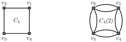
At this point we need to introduce some definitions. Given a simple graph G and a natural number
l ≥ 1, the l-duplication of G, denoted by G(l), is the multigraph obtained from G when we replace every edge ofGby l parallel edges. Note thatL(G(l)) =lL(G) for any graphG.
v1
v2
v3 v4
C4
v1
v2
v3 v4
[image:21.612.206.426.514.587.2]C4(2)
Figure I.1: The simple cycle C4 and its 2-duplication.
Given a graphGand a natural numberk, thek-cone ofG, denoted byck(G), is the multigraph obtained
fromGby adding a new vertexsand addingkparallel edges betweensand all the vertices ofG. Note thatL(ck(G), s) =L(G) +kI|V(G)| for any graphG.
v1
v2
v3 v4
C4
s v1
v2
v3 v4
c1(C4)
Figure I.2: The cycleC4 and its 1-cone.
s
v1 v2 vn−1 vn
m m m m
l l
Corollary 2.1. For all m≥ 0, l ≥ 1, and n≥2, let cm(Pn(l)) be the m-cone of the thick path with
all the edges with multiplicities equal to l. Then
K(cm(Pn(l))) =Znr−1⊕Zmfn−1(m+2l,−l)/rn−1,
where r = gcd(l, m).
Proof. Since the reduced Laplacian matrix of cm(Pn(l)), L(cm(Pn(l)), s), is equal to Pn(m+ 2l,−l)
and gcd(m+ 2l,−l) = gcd(l, m) =r, then by Corollary 1.5 (ii) we get the result.
Corollary 2.2. For all m≥0, l≥1, and n≥4, let cm(Cn(l)) be the m-cone of the thick cycle where
s v3
v2
v1
vn
vn−1
vn−2
m m m m m
m l
l
l l
l
all the edges has multiplicity equal to l. Then
K(cm(Cn(l))) =
Znr−2⊕Zrsq ⊕Zmsq if n−2 = 2q+ 1,
Zn−2
r ⊕Zrtq ⊕Zm(m+4l)tq/r if n−2 = 2q and m/r is odd,
Znr−2⊕Z2rtq ⊕Zm(m+4l)tq/2r if n−2 = 2q andm/r is even,
where r = gcd(l, m), sq= (fq+1(m+ 2l,−l) +lfq(m+ 2l,−l))/rq+1, andtq=fq(m+ 2l,−l)/rq.
Corollary 1.5 (iv), Cn(m+ 2l,−l)∼urIn−2⊕C, where
C=
fq(m+ 2l,−l)/rq
m+ 2l −2l
−2l m+ 2l
ifn−2 = 2q,
fq+1(m+ 2l,−l) +lfq(m+ 2l,−l)/rq+1
r 0
0 m
ifn−2 = 2q+ 1.
Finally,
m+ 2l −2l −2l m+ 2l
!
∼u
r 0
0 (m2+ 4ml)/r
ifm/r is odd,
2r 0
0 (m2+ 4ml)/2r
ifm/r is even.
Corollary 2.3. For all m ≥ 0, l ≥ 1, and n ≥4, let cm(Kn(l)) be the m-cone of the thick complete
graph where all the edges have multiplicity equal to l. Then
K(cm(Kn(l))) =Zr⊕Zmn−+2nl⊕Zm(m+nl)/r,
where r = gcd(l, m).
Proof. Since the reduced Laplacian matrix, L(cm(Kn(l)), s), is equal to Kn(m+nl,−l) and gcd(m+
nl,−l) = gcd(l, m) =r, then by Corollary 1.5 (iii) we get the result.
The subring Kn(A)
In this part we will turn our attention to the case whenA is the subring of matrices given by
Kn(A) ={Kn(a, b)|a, b∈A} ⊂Mn(A).
At first, we will prove that Kn(A) is a subalgebra of Mn(A).
Lemma 2.4. If a, b, c, d, α∈A, then
(i) α·Kn(a, b) =Kn(α·a, α·b),
(ii) Kn(a, b) +Kn(c, d) =Kn(a+c, b+d),
(iii) Kn(a, b)·Kn(c, d) =Kn(ac, ad+bc+nbd),
where the polynomialspm,n(x, y)∈A[x, y] satisfy the recurrence relation
pnm(x, y) = (x+ny)pnm−1(x, y) +yxm−1
with initial value pn
0(x, y) = 0.
Proof. The parts (i) and (ii) are straightforward. (iii) SinceA(Kn)2 = (n−1)In+ (n−2)A(Kn), then
Kn(a, b)·Kn(c, d) = ((a+b)In+bA(Kn))·((c+d)In+dA(Kn)) = (ac+ad+bc+nbd)In+ (ad+bc+
nbd)A(Kn) =Kn(ac, ad+bc+nbd).
(iv) We will use induction onm. The result is clear form= 1 becausepn1(a, b) = (a+nb)pn0(a, b)+ba0=
b. Assume that the result is true for all the natural numbers less or equal tom−1. Thus
Kn(a, b)m = Kn(a, b)m−1·Kn(a, b) =Kn(am−1, pnm−1(a, b))·Kn(a, b)
= Kn(am,(a+nb)pnm−1(a, b) +bam−1) =Kn(am, pnm(a, b)).
Remark. Note that Kn(A) is a commutative ring with identity because Kn(1,0) =In for alln∈ N.
On the other hand, sinceKn(0,1)Kn(−n,1) = 0 =Kn(0,0), thenKn(A) is not a principal ideal domain
because it has zero divisors.
Remark. Using induction onn is not difficult to see that
pnm(x, y) =
m
X
i=1
ni−1
m i
xm−iyi.
Also, since pnm(n,−1) = (n−n)pnm−1(n,−1)−(n)m−1=−nm−1, then
Kn(n,−1)m=nm−1Kn(n,−1) for all m∈N.
Now, we will apply Theorem 1.1 (iii) when the base ring is the subring of matrices with entries in
Kn(A) to obtain a theorem that will be a powerful tool to calculate the critical group of several graphs.
GivenA= (ai,j), B= (bi,j)∈Mn(A) and m≥2, let
Φm(A, B) =
Km(a1,1, b1,1) · · · Km(a1,n, b1,n)
..
. . .. ...
Km(an,1, bn,1) · · · Km(an,n, bn,n)
∈Mn(Km(A))⊆Mnm(A).
As the next theorem will show, if a matrix has the block structure of Φm(A, B), then we can get a
simpler equivalent matrix.
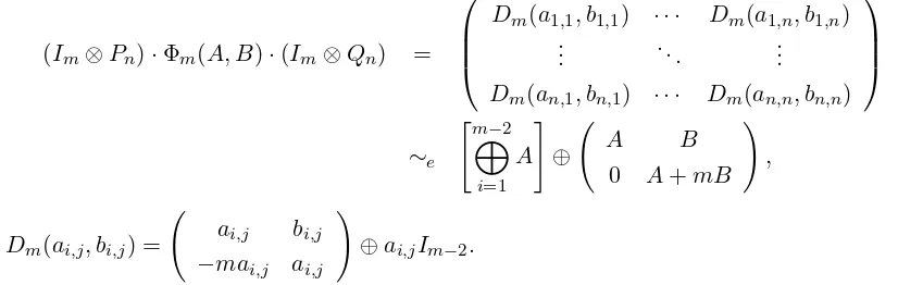
Theorem 2.5. Let A= (ai,j), B= (bi,j)∈Mn(A) and n≥2, then
Φm(A, B)∼e
"m−2 M
i=1
A
#
⊕ A B
0 A+mB
Proof. Let Pn and Qn be as in Claim 1.3, thenIm⊗Pn, Im⊗Qn ∈Mnm(A) are elementary matrices
and
(Im⊗Pn)·Φm(A, B)·(Im⊗Qn) =
Dm(a1,1, b1,1) · · · Dm(a1,n, b1,n)
..
. . .. ...
Dm(an,1, bn,1) · · · Dm(an,n, bn,n)
∼e
"m−2 M
i=1
A
#
⊕ A B
0 A+mB
!
,
whereDm(ai,j, bi,j) =
ai,j bi,j
−mai,j ai,j
!
⊕ai,jIm−2.
In the last part of this paper, we will use Theorem 2.5 in order to find the critical group of some graphs whose Laplacian matrix is given by Φm(A, B) for some A, B ∈ Mn(A). The simplest case is
when n= 2. If Φm(A, B) is the Laplacian matrix of a graph, then the vertex set of the graph can be
partitioned in two sets and the incidence structure between these sets is given by a matrix in Km(Z).
In this sense, we will define the following families of graphs:
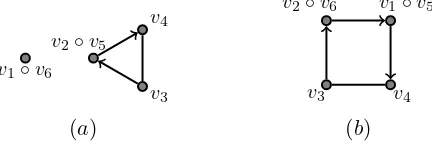
Let U ={u1, u2, . . . , um}, V ={v1, v2, . . . , vm}, and Xy,z be the graph withU ∪V as vertex set and
edge set equal toEy∪Ez∪Ey,z, where
Ey =
∅ ify=m,
uiuj for all i6=j∈ {1,2,· · · , m} ify=M,
similarly forEz, and
Ey,z =
uiu′j for all i, j∈ {1,2,· · · , m} ifX =K,
uiu′j for all i6=j∈ {1,2,· · ·, m} ifX =L,
uiu′i for all i∈ {1,2,· · ·, m} ifX =M.
Note that Km,m is the bipartite complete graph with m vertices in each partition and Lm,m is the
bipartite complete graph with 2mvertices minus a matching. The Laplacian matrix of all these graphs can be represented by Φm(A, B) for some two by two matricesA andB.
For instance, the graphMM,m is illustrated in Figure I.3.
Km Ey,z
Ey Ez
[image:25.612.101.514.108.239.2]The trivial graph
Figure I.3: The graphMM,m.
Before using Theorem 2.5 in order to calculate the critical group of then-cones of graphsXy,z, we will
introduce a theorem that gives an equivalent matrix ofXy,z when the base ring is a general commutative
Corollary 2.6. Let m ≥ 2, a, b ∈ A such that the equation ax+by = 1 has a solution in A, and
Xy,y(a, b) =aI2m+bA(Xy,y). Then
(i) Km,m(a, b)∼uI2⊕aI2(m−2)⊕a
a mb
mb a
!
,
(ii) Lm,m(a, b)∼u Im⊕(a2−b2)Im−2⊕
a2 (m−2)ab
(m−2)ab a2−(m−1)b2 !
,
(iii) LM,M(a, b)∼u Im−1⊕a(a−2b)Im−2⊕
a(a−2b) ab 0
0 a+ 2(m−1)b 0
0 (m−1)b a
,
(iv) MM,M(a, b)∼u Im+1⊕a(a−2b)Im−2⊕
a(a−2b) −b2(2a+ (m−2)b)
0 (a+ (m−1)b)2−b2
!
.
Proof. (i) Since Km,m(a, b) = Φm(A, B) for A=
a 0
0 a
!
and B = 0 b
b 0
!
, then by Theorem 2.5
Km,m(a, b)∼e
"m−2 M i=1 a 0 0 a !# ⊕
a 0 0 b
0 a b 0
0 0 a mb
0 0 mb a
. Moreover, since
a 0 0 b
0 a b 0
0 0 a mb
0 0 mb a
x 0 0 −b
0 1 0 0 0 0 1 0
y 0 0 a
=
1 0 0 0
0 a b 0
mby 0 a mab
ay 0 mb a2
∼e
1 0 0 0
0 a b 0
0 0 a mab
0 0 mb a2
and
a b 0
0 a mab
0 mb a2
x −b 0
y a 0
0 0 1
=
1 0 0
ay a2 mab
mby mab a2
∼e
1 0 0
0 a2 mab
0 mab a2 , then
a 0 0 b
0 a b 0
0 0 a mb
0 0 mb a
∼u I2⊕a
a mb
mb a
!
.
Hence
Km,m(a, b)∼u I2⊕aI2(m−2)⊕a
a mb
mb a
!
(ii) SinceLm,m(a, b) = Φm(A, B) forA=
a −b
−b a
!
and B = 0 b
b 0
!
, then by Theorem 2.5
Lm,m(a, b)∼e
"m−2 M i=1 a −b −b a !# ⊕
a −b 0 b
−b a b 0
0 0 a (m−1)b
0 0 (m−1)b a
. Moreover, since a −b −b a ! x b −y a !
= 1 0
−by−ay a2−b2
!
∼e
1 0
0 a2−b2
! ,
a −b 0 b
−b a b 0
0 0 a (m−1)b
0 0 (m−1)b a
∼e
a 0 0 b
−b a b 0
0 (m−1)b a (m−1)b
0 a (m−1)b a
,
1 0 0 0
∗ a b b2
∗ (m−1)b a (m−1)ab
∗ a (m−1)b a2
=
a 0 0 b
−b a b 0
0 (m−1)b a (m−1)b
0 a (m−1)b a
x 0 0 −b
0 1 0 0 0 0 1 0
y 0 0 a
∼e I1⊕
a b 0
(m−1)b a (m−2)ab a (m−1)b a2−(m−1)b2
, and
1 0 0
∗ a2 (m−2)ab ∗ (m−2)ab a2−(m−1)b2
=
a b 0
(m−1)b a (m−2)ab a (m−1)b a2−(m−1)b2
x −b 0
y a 0 0 0 1
∼e I1⊕
a2 (m−2)ab
(m−2)ab a2−(m−1)b2
!
,
then
Lm,m(a, b)∼u Im⊕(a2−b2)Im−2⊕
a2 (m−2)ab
(m−2)ab a2−(m−1)b2 !
.
(iii) SinceLM,M(a, b) = Φm(A, B) forA=
a−b −b
−b a−b
!
andB = b b
b b
!
, then by Theorem 2.5
LM,M(a, b)∼e
"m−2 M
i=1
a−b −b
−b a−b
!# ⊕
a−b −b b b
−b a−b b b
0 0 a+ (m−1)b (m−1)b
0 0 (m−1)b a+ (m−1)b
Moreover, since
x −(x+y)
b a−b
!
a−b −b
−b a−b
!
= 1 ∗
0 a(a−2b) !
∼e
1 0
0 a(a−2b) !
,
x −(x+y) 0
b a−b 0
0 0 I2
a−b −b b b
−b a−b b b
0 0 a+ (m−1)b (m−1)b 0 0 (m−1)b a+ (m−1)b
=
1 ∗ ∗ ∗
0 a(a−2b) ab ab
0 0 a+ (m−1)b (m−1)b 0 0 (m−1)b a+ (m−1)b
, and
a(a−2b) ab ab
0 a+ (m−1)b (m−1)b
0 (m−1)b a+ (m−1)b
∼e
a(a−2b) ab 0
0 a+ 2(m−1)b 0
0 (m−1)b a
then the result is followed.
(iv) SinceMM,M(a, b) = Φm(A, B) forA=
a−b b
b a−b
!
andB = b 0 0 b
!
, then by Theorem 2.5
MM,M(a, b)∼e
"m−2 M
i=1
a−b b
b a−b
!# ⊕
a−b b b 0
b a−b 0 b
0 0 a+ (m−1)b b
0 0 b a+ (m−1)b
. Moreover, since
x x+y 0
−b a−b 0
0 0 I2
a−b b b 0
b a−b 0 b
0 0 a+ (m−1)b b
0 0 b a+ (m−1)b
=
1 ∗ ∗ ∗
0 a(a−2b) −b2 (a−b)b
0 0 a+ (m−1)b b
0 0 b a+ (m−1)b
and
a(a−2b) −b2 (a−b)b
0 a+ (m−1)b b
0 b a+ (m−1)b
1 0 0
0 a+ (m−1)b y−(m−1)x
0 −b x
=
a(a−2b) −b2(2a+ (m−2)b) ∗
0 (a+ (m−1)b)2− b2 ∗
0 0 1
,
then the result is followed.
Remark. Note that KM,M is the complete graph with 2m vertices andMm,m is the disjoint union of
m copies of K2.
When a graphG is not regular, then there is not a straightforward way to define their matrixG(a, b). Thus, we will defineKm,M(a, b) as a(Im⊕2Im) +bA(Km,M),Lm,M(a, b) as a(Im⊕2Im) +bA(Lm,M),
and Mm,M(a, b) as a(Im⊕(m+ 1)Im) +bA(Mm,M). Now, we have the following equivalent matrices
of Km,M(a, b),Lm,M(a, b), andMm,M(a, b).
Corollary 2.7. Let m≥2, a, b∈A such that the equation ax+by= 1 has a solution in A, then
(i) Km,M(a, b)∼u I2⊕aIm−2⊕2aIm−2⊕a
2a −(a−mb)b
2m 2a
!
(ii) Mm,M(a, b)∼u Im⊕((m+ 1)a2−b2)Im−2⊕
(m+ 1)a2−b2 b
0 (a+b)(b−(m+ 1)a) !
,
(iii) Lm,M(a, b)∼uIm−1⊕(2a2−b2)Im−2⊕
2a2−b2 0 ab+mb2
0 a (m−1)b
0 (m−1)b 2a+mb
.
Proof. (i) SinceKm,M(a, b) = Φm(A, B) for A=
a 0
0 2a
!
and B = 0 b
b b
!
, then by Theorem 2.5
Km,M(a, b)∼e
"m−2
M a 0
0 2a
!# ⊕
a 0 0 b
0 2a b b
0 0 a mb
0 0 mb 2a+mb
. Moreover,
a 0 0 b
0 2a b b
0 0 a mb
0 0 mb 2a+mb
x 0 0 −b
0 1 0 0 0 0 1 0
y 0 0 a
=
1 0 0 0
∗ 2a b ab
∗ 0 a mab
∗ 0 mb 2a2+mab
∼e
1 0 0 0
0 b 2a ab
0 a 0 mab
0 0 −2ma 2a2
and
y x 0
−a b 0
0 0 1
b 2a ab
a 0 mab
0 −2ma 2a2
=
1 ∗ ∗
0 −2a2 mab2−a2b
0 −2ma 2a2
∼eI1⊕
2a2 ab(mb−a) 2ma 2a2
!
.
(ii) SinceMm,M(a, b) = Φm(A, B) forA=
a b
b (m+ 1)a
!
andB= 0 0 0 b
!
, then by Theorem 2.5
Mm,M(a, b)∼
"m−2
M a b
b (m+ 1)a
!# ⊕
a b 0 0
b (m+ 1)a 0 b
0 0 a b
0 0 b (m+ 1)a+mb
Moreover, a b
b (m+ 1)a
!
x −b
y a
!
= 1 0
∗ (m+ 1)a2−b2 !
∼e
1 0
and
a b 0 0
b (m+ 1)a 0 b
0 0 a b
0 0 b (m+ 1)a+mb
∼u
1 0 0 0
∗ (m+ 1)a2−b2 0 b
∗ 0 a b
∗ 0 b (m+ 1)a+mb
∼e I1⊕
b (m+ 1)a+mb 0
a b 0
0 b (m+ 1)a2−b2
∼u I2⊕
(a+b)(b−(m+ 1)a) 0
b (m+ 1)a2−b2
!
(iii) Since Lm,M(a, b) = Φm(A, B) for A=
a −b
−b 2a
!
and B = 0 b
b b
!
, then by Theorem 2.5
Lm,M(a, b)∼
"m−2
M a −b
−b 2a
!# ⊕
a −b 0 b
−b 2a b b
0 0 a (m−1)b
0 0 (m−1)b 2a+mb
. Moreover, x −y b a ! a −b
−b 2a
!
= 1 ∗
0 2a2−b2 !
∼e
1 0
0 2a2−b2 ! ,
a −b 0 b
−b 2a b b
0 0 a (m−1)b
0 0 (m−1)b 2a+mb
∼u
1 0 0 0
0 2a2−b2 ab ab+b2
0 0 a (m−1)b
0 0 (m−1)b 2a+mb
, and
2a2−b2 ab ab+b2
0 a (m−1)b
0 (m−1)b 2a+mb
∼e
2a2−b2 0 ab+mb2
0 a (m−1)b
0 (m−1)b 2a+mb
.
The next corollaries calculate the critical group of then-cone of the graphsXy,z.
Corollary 2.8. Let m≥2, l≥1, and n≥0, then
K(cn(Km,m(l))) =Z2r⊕Z
2(m−2)
n+ml ⊕Z(n+ml)s/r⊕Zn(n+ml)(n+2ml)/rs,
Proof. Since L(cn(Km,m(l)), s) =Km,m(n+ml,−l) andKm,m(n+ml,−l) =rKm,m((n+ml)/r,−l/r)
with gcd((n+ml)/r,−l/r) = 1, then applying Corollary 2.7 (i) toKm,m((n+ml)/r,−l/r) we get that
Km,m(n+ml,−l)∼u rI2⊕(n+ml)I2(m−2)⊕((n+ml)/r)
n+ml −ml
−ml n+ml
!
.
On the other hand,
n+ml −ml
−ml n+ml
!
∼u
s 0
0 n(n+ 2ml)/s
!
,
wheres= gcd(ml, n) and we get the result.
Remark. Note thatKm,mis the complete bipartite graph withmvertices in each partition. Lorenzini
in [31] calculated that
K(Km,m) =Z2(mm−2)⊕Zm2,
which agrees with the Corollary 2.8 for l= 1 and n= 0. Also note that K(cn(Km,m(l))) has 2m−2
invariant factors different to 1.
Corollary 2.9. Let m≥3, l≥1, and n≥0, then
K(cn(Lm,m(l))) =Zmr ⊕Zm(s−2−2l2)/r⊕Zrt⊕Zu/r3t,
where r= gcd(l, n),s=n+ (m−1)l,t= gcd(m−1, n)/gcd(l, m−1, n), and u=s2(n2+ 2n(m−1)l+ (m−2)l2).
Proof. In a similar way that in Corollary 2.8,L(cn(Lm,m(l)), s) =Lm,m(n+ (m−1)l,−l) and applying
Corollary 2.7 (ii) to Lm,m(a/r, b/r) witha=n+ (m−1)l and b=−l
Lm,m(n+ (m−1)l,−l)∼urIm⊕(s2−l2)/rIm−2⊕
a2/r (m−2)ab/r
(m−2)ab/r (a2−(m−1)b2)/r
!
,
wheres=n+ (m−1)l.
On the other hand, it is not difficult to see that
a2/r (m−2)ab/r
(m−2)ab/r (a2−(m−1)b2)/r
!
∼u
rt 0
0 u/r3t
!
,
wheret= gcd(m−1, n)/gcd(l, m−1, n) and u=s2(n2+ 2n(m−1)l+ (m−2)l2).
Corollary 2.10. Let m≥2, l≥1, andn≥0, then
K(cn(LM,M(l))) =Zmr−1⊕Zmst/r−2⊕Zu⊕Zsv/u⊕Znst/rv,
Proof. SinceL(cn(LM,M(l)), s) =LM,M(n+2(m−1)l,−l) andr= gcd(n+2(m−1)l,−l), then applying
Corollary 2.7 (iii) to LM,M(a/r, b/r) witha=n+ 2(m−1)land b=−lwe get that
LM,M(n+ 2(m−1)l,−l)∼u rIm−1⊕st/rIm−2⊕
st/r −sl/r 0
0 n 0
0 −(m−1)l s
,
wherer = gcd(l, n), s=n+ 2(m−1)l, andt=n+ 2ml. On the other hand, it is not difficult to see that
a(a−2b)/r ab/r 0
0 a+ 2(m−1)b 0
0 (m−1)b a
=
st/r −sl/r 0
0 n 0
0 −(m−1)l s
∼u u⊕sv/u⊕nst/rv,
whereu= gcd(n,(m−1)l) and v= gcd(n,2(m−1)l2/r).
Corollary 2.11. Let m≥2, l≥1, andn≥0, then
K(cn(MM,M(l))) =Zrm+1⊕Zm(n−+2ml)(n+(m+2)l)/r⊕Zu⊕Zn(n+2l)(n+ml)(n+(m+2)l)/ur2,
where r = gcd(l, n), u= gcd(n(n+ 2l), lv(n+t))/r, and v= gcd(m, l/r).
Proof. Since L(cn(MM,M(l)), s) = MM,M(n+ml,−l) andr = gcd(n+ml,−l), then applying
Corol-lary 2.7 (iii) to MM,M(a/r, b/r) witha=n+ml and b=−l we get that
MM,M(n+ml,−l)∼urIm+1⊕st/rIm−2⊕
st/r −l2(n+t)/r2
0 n(n+ 2l)/r,
!
wherer = gcd(l, n), s=n+ml, and t=n+ (m+ 2)l. On the other hand, it is not difficult to see that
st/r −l2(n+t)/r2
0 n(n+ 2l)/r
!
∼u u⊕stn(n+ 2l)/ur2,
whereu= gcd(n(n+ 2l), lv(n+t))/rand v= gcd(m, l/r).
Remark. Note that MM,M(l) is the cartesian product of K2(l) and Kn(l). A deep analysis of the
cartesian product of matrices can be found in [19].
Corollary 2.12. Let m≥2, l≥1, andn≥0, then
K(cn(Km,M(l))) =Zmml−+2n⊕Zm2ml−2+n⊕Z2r⊕Zs(n+2ml)/r2 ⊕Zn(n+ml)(n+2ml)/s,
Proof. Since L(cn(Km,M(l))) = Φm(A, B) for A=
ml+n 0
0 2ml+n
!
and B= 0 −l
−l −l
!
, then
the result is followed by Theorem 2.7 (iv) because
ml+n 0 0 −l
0 2ml+n −l −l
0 0 ml+n −ml
0 0 −ml ml+n
∼u rI2⊕(n+ 2ml)s/r2⊕n(n+ml)(n+ 2ml)/s,
wherer = gcd(l, n) and s= gcd(n2, mlr).
Remark. Note that Km,M is the graph K2m \ Km. In general the expression for K(cn(Km,M(l)))
given in Corollary 2.12 does not give us the invariant factors of K(cn(Km,M(l))). Also note that
K(cn(Km,M(l))) has 2m−2 invariant factors different to 1.
Corollary 2.13. Let m≥2, l≥1, andn≥0, then
K(cn(Mm,M(l))) =Zmr +1⊕Zms/r−2⊕Zn(n+2l)s/r3,
where r = gcd(l, n) and s=n2+ml2+nl(m+ 2).
Proof. Since L(cn(Mm,M(l))) = Φm(A, B) for A =
l+n −l
−l (m+ 1)l+n
!
and B = 0 0 0 −l
!
,
then the result is followed by Theorem 2.7 (v) because
l+n −l
−l (m+ 1)l+n
!
∼ur⊕s/r
and
l+n −l 0 0
−l (m+ 1)l+n 0 −l
0 0 l+n −l
0 0 −l l+n
∼u rI3⊕n(n+ 2l)s/r3,
wherer = gcd(l, n) and s=n2+ml2+nl(m+ 2).
We conclude the chapter with the critical group of the graphLm,M.
Corollary 2.14. Let m≥2, l≥1, andn≥0, then
K(Lm,M) =Zmr ⊕Zms/r−2⊕Zt⊕Zn(n+2(m−1)l)s/tr2,
where r = gcd(l, n), s=n2+ (3m−2)nl+m(2m−3)l2, and t= gcd(n, l3(m−1)(2m−3)/r2).
Proof. Since L(cn(Lm,M(l))) = Φm(A, B) for
A= (m−1)l+n l
l (2m−1)l+n
!
and B = 0 −l
−l −l
!
then the result is followed by Theorem 2.7 (vi) because
(m−1)l+n l
l (2m−1)l+n
!
∼r⊕s/r,
wherer = gcd(l, n), s=n2+ (3m−2)nl+m(2m−3)l2, and
(m−1)l+n l 0 −l
l (2m−1)l+n −l −l
0 0 (m−1)l+n −(m−1)l
0 0 −(m−1)l (m−1)l+n
∼urI2⊕t⊕n(n+ 2(m−1)l)s/tr2,
If XG = {xu|u ∈ V(G)} is the set of variables indexed by the vertices of the graph G, then the
generalized Laplacian matrix ofG, denoted by L(G, XG), is given by
L(G, XG)u,v =
xu ifu=v,
−m(u,v) otherwise.
Furthermore, if P is a commutative ring with identity, P[XG] is the polynomial ring over P in the
variables XG and 1≤i≤n, then thei-critical idealof Gis the determinantal ideal given by
Ii(G, XG) =hminorsi(L(G, XG))i ⊆ P[XG],
where minorsi(L(G, XG)) is the set of determinants of all the i-square submatrices of L(G, XG). Note
that we can define (without any technical issue) the critical ideals of an n×n matrixM with entries inP asIi(M, X) =hminorsi(L(M, X))i ⊆ P[X] for alli= 1, . . . , n, where
L(M, X)u,v =
xu ifu=v,
−Mu,v otherwise.
The critical ideals and the critical group of a graph are closely related, as Propositions 1.6 and 1.7 show. Moreover, critical ideals of a graph are very useful to get a better understanding of its critical group. In Section 1, we will show that the critical ideals are better behaved than the critical group. For instance, ifγP(G) is the number of critical ideals over the base ringP that are trivial, then Theorem 1.12 asserts
that
γP(G)≤2(|V(G)| −α(G)) andγP(G)≤2(|V(G)| −ω(G)) + 1,
whereα(G) is the stability number andω(G) is the clique number of the graph. That is; the invariant
γP is closely related to the combinatorics of the graph. Also, ifH is an induced subdigraph ofG, then
γP(H) ≤γP(G) in contrast with the behavior of the number of invariant factors equal to one of the
critical group of induced subdigraphs.
and we define the invariantγP as the number of the critical ideals that are trivial. Also, in this section
we get the reduced Gr¨obner basis of the complete graph. Finally, we explore the relationship of the critical ideals of a graph with the characteristic polynomial of its adjacency and Laplacian matrices. The reduced Gr¨obner basis of the critical ideals of the cycles and some combinatorial expression for the minors of the generalized Laplacian matrix of a digraph are presented in Section 2.
1. Critical ideals of graphs
In this section, we introduce the main concept of this chapter: the critical ideals of a digraphG. We will begin this section by defining the critical ideals of a digraph, presenting some examples and discussing some of their basic properties. In general terms, the i-th critical ideal is the determinantal ideal of
i-minors of the generalized Laplacian matrix associated toG. The critical ideals of G generalize the critical group of G (see Proposition 1.6) and the characteristic polynomials of the adjacency matrix and the Laplacian matrix associated toG(see Section ). Moreover, with some additional requirements overGwe can get a stronger correspondence between the critical ideals of Gand the critical group of
G, see Proposition 1.7.
Afterward, we introduce the number of critical ideals that are trivial as an invariant of the digraph. In the case of graphs, we will establish a bound between this invariant and the stability and clique numbers of the graph. Also, in Section we present a minimal set of generators and a reduced Gr¨obner basis for the critical ideals of the complete graphs. As a byproduct we will get expressions for the critical groups for a complete graph minus a star. Finally, we will explore the relation between the critical ideals of a graph and the characteristic polynomial of its adjacency and Laplacian matrix.
Definition 1.1. Given a digraph Gwith nvertices and 1≤i≤n, let
Ii(G, X) =hminorsi(L(G, X))i ⊆ P[XG]
be the i-th critical ideal of G.
Note that in general the critical ideals depend on the base ring P, in this chapter we are mainly interested when P =Z. By convention, Ii(G, X) =h1i if i≤ 0 and Ii(G, X) = h0i ifi > n. Clearly
In(G, X) is a principal ideal generated by the determinant of the generalized Laplacian matrix.
Now, we present an example that illustrates the concept of critical ideal.
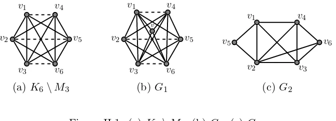
Example 1.2. LetH be the complete graph with six vertices minus the perfect matching formed by the edges M3={v1v4, v2v5, v3v6}(see Figure II.1(a)) andP =Z. Then,
L(H, X) =
x1 −1 −1 0 −1 −1
−1 x2 −1 −1 0 −1
−1 −1 x3 −1 −1 0
0 −1 −1 x4 −1 −1
−1 0 −1 −1 x5 −1
−1 −1 0 −1 −1 x6
Using any algebraic system, for instance Macaulay 2, it is not difficult to see that Ii(H, X) =h1i for
i= 1,2 and
Ii(H, X) =
2, x1, x2, x3, x4, x5, x6 ifi= 3,
{xrxs|vrvs∈E(H)} ∪ {2xr+ 2xs+xrxs|vrvs6∈E(H)} ifi= 4,
{xkxl(xr+xs+xrxs)|(r, s, k, l)∈S(H)} ∪ {p(r,s,k,l)|vrvs, vkvl 6∈E(H)}
ifi= 5,
x1x2x3x4x5x6−P(r,s,k,l)∈S(H)xrxsxkxl−2P(r,s,k)∈T(H)xrxsxk ifi= 6,
where
S(H) ={(r, s, k, l)|vrvs6∈E(H), vkvl∈E(H), and {i, j} ∩ {k, l}=∅},
T(H) are the triangles of H, andp(r,s,k,l)= (xr+xs)(xk+xl+xkxl) + (xk+xl)(xr+xs+xrxs). Note
that the expressions of the critical ideals of H depend heavily on their combinatorics.
Now, let us turn our attention to one of the most basic properties of the critical ideals.
Proposition 1.3. If Gis a digraph with nvertices, then
h0i(In(G, X)⊆ · · · ⊆I2(G, X)⊆I1(G, X)⊆ h1i.
Moreover, if H is an induced subdigraph of G with m vertices, then Ik(H, X) ⊆Ik(G, X) for all1 ≤
k≤m.
Proof. Let M be a (k+ 1)×(k+ 1) matrix over P[XG]. Since det(M) = Pki=1+1Mi,1det(M(i; 1)),
Ik+1(G, X) ⊆Ik(G, X) for all 1≤ k≤n−1. On the other hand, since any submatrix of L(H, X) is
also a submatrix of L(G, X), minorsk(L(H, X)) ⊆minorsk(L(G, X)) for all 1≤ k≤m and therefore
Ik(H, X)⊆Ik(G, X) for all 1≤k≤m.
v5
v4
v1
v2
v3 v6
v5
v4
v1
v2
v3 v6
v
v1
v2 v3
v4
v5 v6
[image:37.612.149.485.476.597.2](a)K6\M3 (b) G1 (c)G2
Figure II.1: (a) K6\M3, (b)G1, (c) G2.
If the digraph is not connected, then we can express its critical ideals as a function of the critical ideals of its connected components.
Proposition 1.4. If Gand H are vertex disjoint digraphs, then
Ii(G⊔H, X) =
* i [
j=0
Ij(G, X)Ii−j(H, X)
+
Proof. Let Q =M⊕N where M ∈Mm(P[X]) and N ∈ Mn(P[X]), k ∈[m+n], and r,s ⊆[m+n]
with|r|=|s|=k. It follows by using induction on |rm|, that
det(Q[r;s]) =
det(Q[rm;sm])·det(Q[rn;sn]) if|rm|=|sm|,
0 otherwise,
whererm =r∩[m],sm=s∩[m], rn=r\rm, andsn=s\sm.
Now, sinceL(G⊔H, X) =L(G, X)⊕L(H, X), we get that minorsi(L(G⊔H, X))\0⊆ {m1·m2|m1 ∈
minorsj(L(G, X)) andm2 ∈minorsi−j(L(H, X)) for some 0 ≤ j ≤i} for all 1 ≤i≤ |V(G∪H)| and
the result is obtained.
Let Tv be the trivial graph composed by the vertex v. Since I1(Tv) =hxvi, applying Proposition 1.4,
we get the critical ideals of the trivial graph with nvertices.
Corollary 1.5. If n≥1 andTn is the graph with n isolated vertices, then
Ii(Tn) ={
Y
j∈J
xj|J|=i} for all1≤i≤n.
Now, we will establish some basic relationships between the critical ideals and the critical group. Before doing this, we will introduce some notation. Given a digraph G with n vertices and d ∈ PV(G), let
L(G,d) be the matrix obtained from L(G, X) where we put xv = dv for all v ∈ V(G). Also, for all
1≤i≤n, let
Ii(G,d) ={f(d)|f ∈Ii(G, X)} ⊆Z.
Given an induced subdigraph H of G, the degree vector of H inG is given by dG(H)v = deg+G(v) for
all v∈V(H).
Proposition 1.6. Let P = Z and G be a digraph (possibly with multiple edges) with n vertices. If
K(G)∼=Lin=1−1Zfi with f1| · · · |fn−1, then
Ii(G, dG(G)) =h i
Y
j=1
fji for all1≤i≤n−1.
Proof. ClearlyL(G, dG(G)) is equal to the Laplacian matrixL(G) ofG. Thus minorsi(L(G, dG(G))) =
minorsi(L(G)) for all 1≤i≤nand therefore
Ii(G, dG(G)) =hminorsi(L(G, dG(G)))i=hminorsi(L(G))i=h i
Y
j=1
fji for all 1≤i≤n−1.
Proposition 1.7. Let P =Z,G be a connected digraph (possibly with multiple edges) with n vertices, andv a vertex of G. If Gis Eulerian (that is,d+G(v) =d−G(v) for all v∈V(G)) andK(G)=∼Lni=1−1Zfi
with f1| · · · |fn−1, then
Ii(G\v, dG(G\v)) =h i
Y
j=1
fji for all1≤i≤n−1.
Proof. Since L(G\v, dG(G\v)) =L(G, v) (the reduced Laplacian matrix ofG), by Proposition 1.6 we
only need to prove that K(G) ∼=ZV(G)\v/ImL(G, v)t. Now, if In−1,n−1 is the identity matrix of size
n−1, then
"
1 1
0 In−1,n−1 #
L(G) "
1 1
0 In−1,n−1 #t
= 0⊕L(G, v).
Since det( "
1 1
0 In−1,n−1 #
) = 1, thenL(G)∼0⊕L(G, v) and we get the result.
Remark. Note that, in general, Proposition 1.7 is not valid for digraphs. However, we can get a similar result for matrices inMn×nwith entries in a principal ideal domain and such thatM1=0 and
1M =0.
The next example shows how Proposition 1.7 can be used to recover the critical group of a graph from its critical ideals. In this sense, critical ideals generalize the critical group of a graph.
Example 1.8. Let H be the complete graph with six vertices minus a perfect matching as in Fig-ure II.1(a). andGbe a graph such thatH=G\vfor some vertexvofG. Thus, applying Proposition 1.7 we can get the critical group ofGas an evaluation of the critical ideals ofH. For instance, ifG1 is the
graph obtained from H (see Figure II.1(b)) by adding a new vertexv and the edges vv1, vv3, vv4, vv6,
then dG(H) = (5,4,5,5,4,5). Moreover, using the critical ideals of H calculated in Example 1.2, we
get that fi= 1 for all i≤4, f5= 20, f6 = 140; that is,
K(G1)∼=Z20⊕Z140.
On the other hand, if we only know the critical ideals of induced subgraphs of G that are different to
G\v, then we cannot reconstruct completely the critical group ofG. For instance, if G2 is the graph
obtained by adding the vertices v5, v6 and the edges v5v1, v5v2, v6v2, v6v3, v6v4 to the complete graph
with four vertices (see Figure II.1(c)), then it is not difficult to see using any algebraic system that
fi(G2) = 1 for 1 ≤i ≤4 and f5(G2) = 185. However, when we apply Proposition 1.7 to the critical
ideals of the induced subgraph by the verticesv1,v2,v3, andv4 ofG2 (isomorphic toK4) we can only
obtain thatf1(G2) =f2(G2) = 1, f3(G2)|5 andf4(G2)|175.
The invariant γ
Definition 1.9. Given a digraph Gand a commutative ring with identity P, let
γP(G) = max{i|Ii(G, X) =h1i}.
Using the canonical homomorphisms f : Z → P given by f(a) = af(1) is not difficult to get that
γZ(G) ≤ γP(G). For instance, it is clear that γZ(G) ≤ γQ(G). Also, there exists a close relation
betweenγZ(G) and the number of invariant factors of the critical group of Gthat are equal to 1. For
instance, if IF1(G) denote the number of invariant factors of the critical group of Gthat are equal to
1, thenγZ(G)≤IF1(G). We found thatγP(G) behaves better than the number of invariant factors of
the critical group of a digraph that are one. For instance, it is not difficult to see from the definition and Proposition 1.3 that if H is an induced subdigraph of G, then γP(H) ≤ γP(G). However, if
n ≥ 3, G = K2,n is a complete bipartite graph, and H = K1,n is an induced subgraph of G, then
IF1(G) = 2< n=IF1(H).
Now, we present a relation betweenγP(G) and the stability and the clique numbers ofG. Before doing
this, we will define the stability and the clique numbers of a graph. A subset S of the vertices of a graph G is calledstable or independentif there is no edge of G with ends in S. A stable set is called
maximal if it is under the inclusion of sets. Thestability numberof G, denoted by α(G), is given by
α(G) = max{|S| |S is a stable set of G}.
In a similar way, a subset C of the vertices of a graph Gis called a cliqueif all the pairs of vertices in
C are joined by an edge ofG. A clique set is called maximal if it is under the inclusion of sets. The
clique numberof G, denoted byω(G), is given by
ω(G) = max{|C| |C is a clique set ofG}.
Lemma 1.10. If G is a digraph (possibly with multiple edges) andv is a vertex ofG, then
γP(G)−γP(G\v)≤2.
Proof. We begin with a simple relation between the critical ideals of Gand G\v.
Claim 1.11. If G is a digraph (possibly with multiple edges) with V(G) ={v1, . . . , vn}, then
Ij(G, X)⊆ hx1Ij−1(G\v1, X\x1), Ij−2(G\v1, X\x1)i for all1≤j≤n.
Proof. Let I = {i1, . . . ij} ⊆ [n], I′ = {i′i, . . . , i′j} ⊆ [n] and mI,I′ = det(L(G, X)[I, I′]) ∈ Ij(G). If 1∈/I∪I′, thenmI,I′ ∈Ij(G\v1, X\x1). In a similar way, if 1∈I∆I′, thenmI,I′ ∈Ij−1(G\v1, X\x1). On the other hand, if 1∈I∩I′, then
mI,I′ ∈ hx1Ij−1(G\v1, X\x1), Ij−2(G\v1, X\x1)i.
Letg=γP(G\v1). Since Ii(G\v1, X\x1)6=h1i for all i≥g+ 1, by Claim 1.11
Ig+3(G, X)⊆ hx1Ig+2(G\v1, X\x1), Ig+1(G\v1, X\x1)i 6=h1i.
ThereforeIg+3(G, X)6=h1i. That is, γP(G)−γP(G\v1)≤2.
Since γP(Tm) = 0 and γP(Kn+1) = 1 for all m, n ≥1, then using Lemma 1.10 we have the following
result:
Theorem 1.12. If G is a digraph (possibly with multiple edges) withn vertices, then
γP(G)≤2(n−ω(G)) + 1and γP(G)≤2(n−α(G)).
Proof. The result follows by using that γP(Tα(G)) = 0 (Corollary 1.5), γP(Kω(G)) = 1 (Theorem 1.15)
and the fact that γP(G)−γP(G\v)≤2 for allv∈V(G) (Lemma 1.10).
This result is interesting when the stability or the clique number is almost the number of vertices of the graph. For instance, ifGis the complete graph (ω(G) =n), thenγP(G)≤1. Theorem 1.15 proves
that this bound is tight. Similarly to Theorem 1.12, in [31] an upper bound for the number of invariant factors different to one of the critical group of a graphGin terms of the number of independent cycles of Gwas found.
In [29] a similar result to the obtained in the proof of Theorem 1.12 was obtained. Namely in [29] it was shown that ifG is a simple graph ande∈E(G), then the number of invariant factors different to 1 ofG andG\ediffer by at most 1.
Clearly, a simple graphG hasγP(G) = 0 if and only if Gis the trivial graph. Moreover, in [4] it was
shown that a simple graphGhasγZ(G) = 1 if and only ifGis the complete graph. Also, all the simple
graphs withγZ equal to 2 were characterized in [4].
It is not difficult to prove that the bound γP(G) ≤ 2(n−α(G)) is tight. For instance, it is easy to
prove that ifP2n+1 is an odd path (see Corollary 2.8), thenα(P2n+1) =n+ 1 andγP(P2n+1) = 2n=
2(2n+ 1−(n+ 1)). Moreover, in Chapter III it was shown that if T is a tree, thenγZ(T) is equal to
its 2-matching number. This result proves that the boundγP(G)≤2(n−α(G)) is tight for any value
of the stability number and the number of vertices of the graph. An interesting open question is the characterization of the simple graphs that satisfy the bounds given in Theorem 1.12.
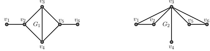
Next example shows a graphGwith γZ(G) = 5 such thatL(G, X) has no 5-minor equal to 1.
Example 1.13. LetG be the cone of H (obtained from H when we add a new vertex v and all the edges between the vertex v and the vertices of H), see Figure II.2. Since
det(L(G, X)[{1,2,3,4,5},{2,3,5,6,7}]) =x2+x5+x2x5 and
det(L(G, X)[{1,2,3,5,6},{2,4,5,6,7}]) =−(1 +x2+x5+x2x5),
then γZ(G) = 5. However, it is not difficult to check that no 5-minor of L(G, X) is equal to one or
another integer.
v1
v2 v3 v4 v5
v6
H
L(c(H), X) =
x1 −1 −1 0 0 −1 −1
−1 x2 −1 0 0 0 −1
−1 −1 x3 −1 0 −1 −1
0 0 −1 x4 −1 −1 −1
0 0 0 −1 x5 −1 −1
−1 0 −1 −1 −1 x6 −1
[image:42.612.115.489.429.593.2]−1 −1 −1 −1 −1 −1 x7
Figure II.2: A graph H with six vertices and the generalized Laplacian matrix of its cone.
Critical ideals of the complete graphs
We begin this subsection with an expression for the determinant of the complete graph.
Proposition 1.14. If Kn is the complete graph with n≥1 vertices, then
det(L(Kn, X)) = n
Y
j=1
(xj + 1)− n
X
i=1 Y
j6=i
(xj + 1).
Proof. We will use induction onn. Forn= 1, it is clear that det(L(Kn, X)) =x1 = (x1+ 1)−1. Now,
assume thatn≥2. Expanding the determinant ofL(Kn+1, X) by the last column and using induction
hypothesis
det(L(Kn+1, X)) = xn+1·det(L(Kn, X)) + n
X
k=1
det(L(Kn, X))xk=−1
= xn+1·
n
Y
j=1
(xj+ 1)− n
X
i=1 Y
j6=i
(xj+ 1)
− n X k=1 Y
j6=k
(xj+ 1)
=
n+1 Y
j=1
(xj+ 1)− n
Y
j=1
(xj+ 1)−(xn+1+ 1)
n
X
i=1 Y
j6=i
(xj+ 1)
=
n+1 Y
j=1
(xj+ 1)− n+1 X
i=1 Y
j6=i
(xj+ 1).
The next result gives us a description of a reduced Gr¨obner basis of the critical ideals of the complete graph.
Theorem 1.15. If Kn is the complete graph with n≥2 vertices and 1≤m≤n−1, then
Bm = Y
i∈I
(xi+ 1)|I ⊆[n] and |I|=m−1