Uncertainty Analysis in Fatigue Design of Offshore Wind Turbine Monopile Structures

(1)

Uncertainty Analysis in Fatigue Design

of Offshore Wind Turbine Monopile

Structures

Daniel Bolado Fernández

Specialization Project in Marine Civil Engineering

Trondheim, December 2018

Supervisor: Michael Muskulus

Norwegian University of Science and Technology Faculty of Engineering

(2)

(3)

I

A

BSTRACT

Importance of offshore wind energy production has grown in the last days. Various types of foundations can be used for offshore wind turbines, being monopile structures the most common solution.

As a result, this project aims to describe the behavior of monopile structures respect to fatigue loads when including uncertainty.

The fatigue design has considered damage equivalent loads (DEL) to obtain damages and probabilities of failure (POF). Monte Carlo method has been used for finding out the effect of the uncertainty of several parameters (natural frequency, damping ratio and sea state) in the POF of the structure.

The results obtained show that natural frequency uncertainty decreases the POF of the structure, while damping ratio uncertainty increases it. The uncertainty in the sea states generation has an almost negligible effect on the POF when having a certain number of simulations performed respect to the use of a scatter diagram.

(4)

(5)

III

T

ABLE OF

C

ONTENTS

ABSTRACT ... I TABLE OF CONTENTS ... III LIST OF FIGURES ... V

1 INTRODUCTION ... 1

1.1 BACKGROUND ... 1

1.1.1 Wind energy ... 1

1.1.2 Offshore wind energy ... 3

1.1.2.1 Offshore support structures ... 4

1.2 PROJECT SCOPE ... 6

2 THEORY ... 7

2.1 WAVE INDUCED FATIGUE LOADS ... 7

2.1.1 Combined transfer function ... 7

2.1.1.1 Hydrodynamic transfer function ... 8

2.1.1.2 Mechanical transfer function ... 8

2.1.1.3 Modal analysis ... 8

2.1.1.4 Damping ratio ... 9

2.1.2 Wave spectrum ... 9

2.2 DAMAGE EQUIVALENT LOADS ... 10

2.3 PROBABILITY OF FAILURE ... 10

2.3.1 Fatigue damage ... 11

2.4 UNCERTAINTY ANALYSIS ... 11

3 METHODOLOGY ... 13

3.1 OBTAINING DAMAGE EQUIVALENT LOADS ... 13

3.1.1 Modal analysis parameters ... 14

3.1.2 Hydrodynamic transfer function ... 14

3.1.3 Tower bending transfer function (HTB) ... 15

3.1.4 Wave spectrum ... 15

(6)

IV

3.2 OBTAINING PROBABILITY OF FAILURE ... 16

3.3 PROBABILITY DENSITY FUNCTIONS IN UNCERTAINTY ANALYSIS ... 18

3.3.1 Natural frequency ... 18

3.3.2 Damping ratio ... 19

3.3.3 Sea state ... 19

4 RESULTS ... 21

4.1 DESIGN WITHOUT CONSIDERING UNCERTAINTY ... 21

4.2 DESIGN WITH UNCERTAINTY IN NATURAL FREQUENCY ... 21

4.3 DESIGN WITH UNCERTAINTY IN DAMPING RATIO ... 22

4.4 DESIGN WITH UNCERTAINTY IN SEA STATES ... 23

5 CONCLUSION ... 25

REFERENCES ... 27

APPENDIX ... 29

MATLAB APPENDIX ... 29

Deterministic program ... 29

Natural frequency uncertainty ... 30

Damping ratio uncertainty ... 32

Sea state uncertainty ... 34

(7)

V

L

IST OF

F

IGURES

FIGURE 1-1: WIND ENERGY CONSUMPTION BY REGION ... 2

FIGURE 1-2: WIND PROFILES DEPENDING ON THE TERRAIN ... 3

FIGURE 1-3: NEW OFFSHORE WIND CAPACITY INSTALLED IN THE WORLD 2000-2020 ... 4

FIGURE 1-4: TYPES OF FOUNDATIONS DEPENDING ON WATER DEPTH ... 5

FIGURE 2-1: JONSWAP SPECTRUM VARIATION WITH FETCH ... 9

FIGURE 2-2: PROBABILITY DENSITY FUNCTION OF FAILURE RESPECT TO DAMAGE ... 11

FIGURE 3-1: POF RESPECT TO DAMAGE ... 17

FIGURE 3-2: PROBABILITY DENSITY FUNCTION OF FM/FD ... 18

FIGURE 3-3: PROBABILITY DENSITY FUNCTION OF DAMPING RATIO ... 19

FIGURE 3-4: CUMULATIVE DENSITY FUNCTION OF SEA STATE ... 20

FIGURE 4-1: RELATIVE DAMAGE RESPECT TO RELATIVE FREQUENCY ... 21

FIGURE 4-2: RELATIVE DAMAGE RESPECT TO RELATIVE DAMPING RATIO ... 22

FIGURE 4-3: PDF OF RELATIVE DAMAGE WITH DAMPING RATIO UNCERTAINTY ... 23

FIGURE 4-4: RELATIVE POF RESPECT TO NUMBER OF SIMULATIONS ... 24

(8)

(9)

Chapter: Introduction Daniel Bolado Fernández

1

1 INTRODUCTION

Design of offshore wind turbine structures is increasing in importance in Europe and in all countries around the world. Offshore structures allow humanity to build huge wind farms far from land. This avoids losing buildable area and also the construction of bigger wind turbines than the ones built onshore.

1.1 B

ACKGROUND

1.1.1 Wind energy

Wind energy is a renewable energy obtained from the wind, but indirectly it has its origin on the sun. Solar radiation is irregularly absorbed by the atmosphere and causes air masses to have different temperatures and densities, changing their pressure. Air moves due to difference in pressure, moving from areas of high pressure to regions of lower pressure. This phenomenon causes wind.

Wind energy is one of the oldest sources of energy ever used. It is thought that first generalized use of wind energy happened around 3,000 BC. Wind was used for propelling Egyptian boats (U.S. Energy Information Administration, 2018).

First wind mills didn´t appear until 500-900 AD in ancient Persia. First windmills were used for grain grinding and water pumping (TelosNet).

In 19th_{century, the invention of the steam engine led to a decrease in the use of windmills. At the}

beginning of the century, Lord Kelvin come up with the idea to couple an electric generator and a wind machine, but it was not doable until the invention of the dynamo in 1850 (Real, Sierra, & Almena, 2016). In 1887, Charles F. Brush built the first wind turbine that could generate energy. The turbine had a 17 m diameter rotor and 144 blades, but it could just generate 12kW.

(10)

2

Fuel-based energy become cheaper than wind production and put wind energy out of the market. However, oil shortage caused countries to look for renewable energy supply solutions. In the 1970s, several countries started national programs to encourage research of energy production through the use of wind turbines (Sørensen, 2011).

Nowadays, wind energy has become a relevant source of power. In 2015, world wind power capacity is 435 GW, what means a 7% of total power capacity (World Energy Council, 2016b). In Europe, 44.2% of all new power installation in 2015 was wind power installations, more than any other form of power generation. At the end of 2015, the EU had 142 GW of installed wind power capacity, 131 GW onshore and 11 GW offshore. Despite that fact, onshore installations decrease by 7.8%, while offshore installations more than doubled, compared to 2014 (World Energy Council, 2016a).

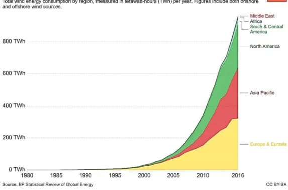
Figure 1-1: Wind energy consumption by region

In the Figure 1-1, it can be seen the importance wind energy has acquired worldwide in the last 30 years. In 1986 wind energy consumption was 0.14 TWh, while in 2016 it was 959.53 TWh. It is important to mention as well that wind energy was a common practice in Europe quite many years ago, but lately it has been highly developed in all regions (Ritchie & Roser, 2018).

(11)

3

Increase in popularity of this source of power have led to an increase in research. That made new solutions, that included more technology and investment, possible for wind turbines.

1.1.2 Offshore wind energy

Offshore wind turbines are a common solution proposed in countries where wind cannot be efficiently exploited on land, but offshore wind turbines are also used in other cases. They present numerous advantages in comparison with onshore ones.

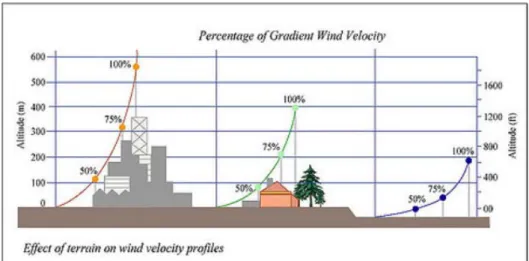
Size of offshore wind turbines is not constrained by capacity limits of available transportation and erection systems and visually, it does not impact the landscape the same way onshore wind turbines do near populated areas. Other benefit of offshore systems is that not that much attention is devoted to reducing noise emissions. Also, offshore wind profile registers higher wind velocities at lower heights than in land due to smaller friction coefficients of the terrain, Figure 1-2 (OpenCourseWare). Higher capacity factors are registered in offshore wind turbines as well.

Figure 1-2: Wind profiles depending on the terrain

Main drawbacks of offshore wind turbine are the high initial investment cost and more difficulties in the design and construction, as well as more severe conditions, corrosion and water loads, that add extra maintenance costs (Musial & Butterfield, 2004).

Offshore wind turbines are a relative new technology. First offshore wind farm was established in the Danish coast in 1991. It was composed by eleven 450 kW turbines for a total capacity of 4.95

(12)

4

MW, the common capacity of just one offshore wind turbine nowadays (European Wind Energy Association, 2011)

Offshore wind technology is a rising trend. 3.3 GW of new offshore wind energy was installed in 2017, making a total cumulative capacity of 17 GW. Europe is the leading region is this technology installing 3.1 GW out of this 3.3 GW last year. Its capacity increased a 25% just in 2017.

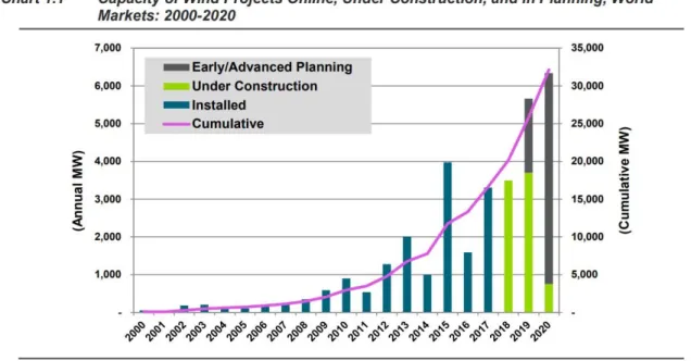
Navigant Research expects over 24 GW of new capacity installed during next 5 years (from 2017 to 2022), which means surpassing 40.6 GW of capacity by 2022. Figure 1-3 shows the expected increase in capacity during the next years (Technica, 2017).

Figure 1-3: New offshore wind capacity installed in the world 2000-2020

1.1.2.1 Offshore support structures

One of the most relevant parts of offshore wind turbines is the selection of the offshore support structure. Its main purpose is to keep the wind turbine on place and it means around a 25% of the total cost of the installation. It has to be able to resist loads in serviceability and ultimate states as well as effects of marine environments, such as corrosion. The support structure also known as foundation has to be able to redirect all loads received into the seabed.

(13)

5

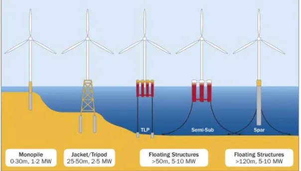
There are different types of support structures available with different characteristics to match site features. Water depth is one of the main variables when deciding which foundations to use. Figure 1-4 shows common foundations used depending on the water depth (Van Der Tempel, 2006).

Figure 1-4: Types of foundations depending on water depth

Monopile structures are used for shallower water depths while jacket and floating solutions are proposed when water depth increases. As a monopile structure is used in this project more background is provided about this type of foundation.

Monopile structures are the most frequently used type of foundation. Ease to produce and install, as well as a wide number of exploitable water depths (up to 30 m), makes this foundation feasible in multiple cases and likely to remain being the most popular solution for offshore design in the near future.

They consist of a foundation pile and a transition piece, where turbine tower is installed. Foundation piles are cylindrical hollow sections made from rolled steel plates welded together. Sometimes transition piece might not even be required, what notably reduces cost. Diameter of monopiles can be up to 6 m and wall thickness as much as 150 mm.

(14)

6

1.2 P

ROJECT SCOPE

The aim of the project is to be able to develop a basic software that permits designing a monopile structure against fatigue failure. To make project more interesting for industry, damage equivalent loads (DEL) method is used for obtaining damage of the structure, what is transformed into the probability of failure of the system (POF).

An uncertainty analysis has been carried out later to consider variability in POF due to change in the variables that affect DEL calculation. Variables analyzed are uncertainty in the damping ratio, sea state and natural frequency of the system.

Several assumptions have been considered and will be detailed in further chapters.

Final purpose of the project is to determine the impact of uncertainty in the fatigue design of a monopile structure and know which variables affect the POF the most and should be considered when designing.

(15)

Chapter: Theory Daniel Bolado Fernández

7

2 THEORY

In order to obtain the fatigue design of monopile structure it is important to know which loads govern the failure process and describe the theory behind them. When monopile structures are used wave induced loads define the behavior of the structure, while wind loads have a negligible effect (Seidel, 2014).

The result of wave loads over the structure, response spectrum, has to be transformed to get DEL to be able to evaluate POF of the structure and the uncertainty analysis.

2.1 W

AVE INDUCED FATIGUE LOADS

Wave loads are usually calculated using frequency domain analysis. General information about this method can be found in (Hapel, 2013) and (Barltrop, 1991).

Frequency domain analysis makes possible to obtain the response spectrum due to wave induced fatigue loads as a combination of the combined transfer function (H(z,ω)) and the wave spectrum (Sξξ(ω)):

𝑆 𝑧, 𝜔 |H z,ω | ∙ S ω

2.1.1 Combined transfer function

Combined transfer function accounts for hydrodynamic transfer function (Ha,n(ω)), mechanical

transfer function (Hn(ω)) and the mode shape (Φn(z)):

(16)

8

2.1.1.1 Hydrodynamic transfer function

Hydrodynamic transfer function includes the effect of inertia and drag forces over the structure in the response of the system.

𝐻 , 𝜔 𝜔 ∙ 𝑐 𝑧 ∙ 𝜂 𝑧, 𝜔 ∙ 𝛷 𝑧 ∙ 𝑑𝑧

𝑖 ∙ 𝜌 ∙ 𝜔 ∙ 𝐶 𝑧 ∙ 𝜋 ∙𝐷 𝑧

4 ∙ 𝜂 𝑧, 𝜔 ∙ 𝛷 𝑧 ∙ 𝑑𝑧

Where, first part of the equation considers drag effect, and second one takes into account inertia effect. Terms would be described in Chapter 3: Methodology, once assumptions have been done.

2.1.1.2 Mechanical transfer function

Mechanical transfer function describes the effect of modal analysis and damping ratio in the response, apart from the mode shape effect:

𝐻 𝜔 1

1 _𝜔𝜔 2 ∙ 𝑖 ∙ 𝜉 ∙ 𝜔_𝜔 ∙ 1 𝐾

2.1.1.3 Modal analysis

Modal analysis is used for obtaining vibration characteristics (natural frequencies and mode shapes) of a structure. Natural frequencies and mode shapes are required when a spectrum analysis is carried out (Ansys guide).

Generalized properties, such as generalized mass (Mn) and generalized stiffness (Kn) can also be

obtained while the analysis is performed. Those variables are necessary for obtaining the response in this project.

For the aim of this project, principle of virtual work has been applied for obtaining the generalized properties as a function of the mode shape (Cangas, 2017):

𝑀 𝑚 𝑧 ∙ 𝛷 𝑧 𝑑𝑧 𝑀 ∙ 𝛷 𝑖

(17)

9

𝐾 𝐸𝐼 𝑧 ∙ 𝛷 𝑧 𝑑𝑧

Where, 𝛷 𝑧 stands for the second derivative of the mode shape respect to x.

Natural frequencies can be obtained easily applying the next equation that relates the main generalized properties already calculated:

𝜔 _𝑀𝐾

If damping ratio is taken into account, the next formula should be used, although normal damping ratio values usually does not really affect modal frequency:

𝜔 , 𝜔 ∙ 1 𝜉

2.1.1.4 Damping ratio

Damping ratio is a dimensionless measure that describes how oscillation amplitude of a system is reduced after an external load created a disturbance. Damping ratio is usually expressed as a percentage of the critical damping, that is the damping that cancel oscillations to reach equilibrium.

2.1.2 Wave spectrum

(18)

10

Spectral analysis makes possible to determine the energy of the waves depending on its frequency, or period, knowing the main spectral characteristics of a sea state.

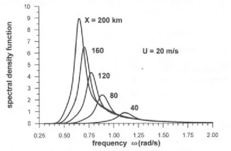
The most used scalar wave spectrum is JONSWAP spectrum, shown in Figure 2-1, especially in offshore constructions. The expression that defines it is (Vidal, 2017):

𝑆 𝑤 𝛼 ∙ 𝑔 ∙ 𝜔 ∙ 𝑒 . ∙ ∙ 𝛾 Where,

𝛿 𝑒 ∙ ∙

𝜎 𝜎 , 𝜔 𝜔

𝜎 , 𝜔 𝜔

α, ωp, γ, 𝜎 , 𝜎 are variables that need to be known for defining the model.

2.2 D

AMAGE EQUIVALENT LOADS

Damage equivalent loads (DEL) remove the variability in moments over the structure and present a moment with constant amplitude through all the time that causes the same damage as the actual loads. DEL are usually adjusted to a frequency of 1 Hz to make calculations simpler.

2.3 P

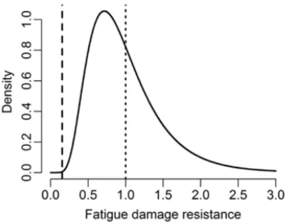
ROBABILITY OF FAILURE

Probability of failure (POF) is defined as the likelihood of a structure to fail. POF depends on multiple variables, however, in this project the damage is going to be the only variable that defines POF. POF density function is shown in Figure 2-2 , obtained from (Muskulus & Schafhirt, 2015). The observed curve is a lognormal distribution with mean equal 1 and a coefficient of variance of 0.50. The broken line points out the fatigue damage that equals a POF of 10-4_{, which is a standard}

value used when designing offshore structures. Dotted line notes the mean value of the POF distribution.

(19)

11

Figure 2-2: Probability density function of failure respect to damage

2.3.1 Fatigue damage

To calculate fatigue damage is necessary to calculate stress range at failure first.

Stress range at failure is calculated using the S-N curve method and following the recommended practices of DNV GL (Veritas, 2010). Stress range must be obtained using the same frequency the DEL were calculated with.

Damage is calculated following Miner’s Rule (Weibull). Substituting number of cycles for the stress range, next formula is obtained:

𝐷𝑎𝑚𝑎𝑔𝑒 𝐶 _𝑆𝑆

Where, S is the stress range obtained by the DEL and Sf is the stress range at failure.

2.4 U

NCERTAINTY ANALYSIS

For the uncertainty analysis Monte Carlo method is going to be used for simplicity. In fact, one of the aims of the project is discover if this method can provide good values with some simulations.

(20)

12

Monte Carlo simulation consists on sampling random values to artificially simulate numerous experiments. To apply Monte Carlo simulation, systematic methods for obtaining random variables are required, as well as an economical and reliable simulation sampling strategy (Melchers & Beck, 2018).

(21)

Chapter: Methodology Daniel Bolado Fernández

13

3 METHODOLOGY

This chapter is used to define how results were obtained through the application of theory. MATLAB was used for obtaining the failure design of the structure and performing Monte Carlo simulations.

3.1 O

BTAINING DAMAGE EQUIVALENT LOADS

Response spectrum has to be transformed to obtain DEL. In (Seidel, 2014), the next simplified formula is obtained: 𝐷𝐸𝐿 1.8825 ∙ S ω ∙𝛷 𝑧 𝐾 ∙ 1 𝜉 ∙ω ∙ 𝐻 , ∙ 𝐻 Where, 𝐻 ω ∙ 𝛷 𝑧 ∙ 𝜇 𝑧 ∙ 𝑧 ∙ 𝑑𝑧

Following assumptions are applied for obtaining this expression:

 Only the first mode is considered for the calculation of the response, wave excitation is outside of the frequency of higher modes.

 Low damping ratio is assumed, 1% is a common value used in monopile structures. This makes possible to assume that the response spectrum in narrow banded and only regions close to natural frequencies are significant. So, functions that included ω as a variable con be calculated just for the case of ω equal to ω0.

 Drag loads are neglected due to huge diameters of monopile structures. This assumption is valid for diameters above 4 m.

(22)

14

 The parameter m, the inverse slope of the S-N curve, is 4, a value in between actual inverse slope values (3 and 5), to consider the variability in the loads over the structure.

In the following sections, it is explained how the unknown values needed for obtaining DEL have been obtained.

3.1.1 Modal analysis parameters

Φ0(z), ω0 and K0 values need to be obtained.

The monopile structure plus the wind turbine is considered as a fixed cantilever with constant diameter, thickness and material properties through all the section with a point load mass on the edge (accounting for nacelle, hub and blades weight) for simplicity. The diameter used for this project is 5 m and 30 mm thickness, obtained considering monopile thickness of around 100 mm thickness and wind turbine tower thickness of some millimeters. The turbine thickness plays a higher impact on the dynamic behavior of the structure, so the thickness is closer to that thickness rather than the monopile one. Assumed material is steel with a specific weight of 78,000 N/m3_and

a Young’s Modulus of 200 GPa. The load mass over the edge of the cantilever has a value of 314,500 kg, obtained from the NREL definition of a 5 MW wind turbine(Jonkman, Butterfield, Musial, & Scott, 2009).

First mode normalized shape (value of 1 at nacelle height (znac)) widely used for the structure and

supports defined above is as follows:

𝛷 𝑧 1 cos _{2 ∙ 𝑧}𝜋 ∙ 𝑧

Once Φ0(z) is defined, values of ω0 and K0 can be obtained with the formulas in Section 2.1.1.3.

3.1.2 Hydrodynamic transfer function

After all made assumptions, hydrodynamic transfer function can be stated as:

𝐻 , 𝜌 ∙ 𝜔 ∙ 𝐶 ∙ 𝜋 ∙𝐷₄ ∙ 𝜂 𝑧 ∙ 𝛷 𝑧 ∙ 𝑑𝑧

Where all variables are known except CM(z) and η0(z). CM(z) is referred as the diffraction correction

(23)

Chapter: Methodology Daniel Bolado Fernández 15 𝐶 2.5 ∙ 𝐷 λ 7.53 ∙ 𝐷 λ 7.9 ∙ 𝐷 λ 3.2 2.0

Where, λ0 is the wave length.

Wave length is obtained through Hunt’s method (U.S. Army Engineer Waterways Experiment Station, 1985), rather than through the exact solution of dispersion equation due to simulation efficiency.

According to Hunt’s method wave length is:

𝐿 𝑇 ∙ 𝑔 ∙ 𝑑 𝐹

Where: T is the wave period, g is the gravity acceleration, d the water depth and F is: 𝐹 𝐺 _1.0 _{0.6522 ∙ 𝐺} _{0.4622 ∙ 𝐺}1 _{0.0864 ∙ 𝐺} _{0.0675 ∙ 𝐺} Being G: 𝐺 2 ∙ 𝜋 𝑇 ∙ 𝑑 𝑔

The following function η0(z) is obtained from linear wave theory.

η z cosh 𝑘 ∙ 𝑧_{sinh 𝑘 ∙ 𝑑} 𝑑

Where, k0 is the wave number obtained dividing 2π over the wave length.

3.1.3 Tower bending transfer function (H

TB

)

HTB is just calculated after all required variables have been obtained in previous sections.

3.1.4 Wave spectrum

As stated in the Chapter 4: Theory, JONSWAP spectrum is used, however, an adaptation of that formula has been used to present it in terms of significant height, Hs, and peak period, Tp, more

(24)

Chapter: Methodology Daniel Bolado Fernández 16 𝑆 𝑓 𝛽 ∙ 𝐻 ∙ 𝑇 ∙ 𝑓 ∙ 𝑒 . ∙ ∙ _{∙ 𝛾} ∙ ∙ Where, 𝛽 0.0624 ∙ 1.094 0.01915 ∙ ln 𝛾 0.230 0.0336 ∙ 𝛾 0.185 ∙ 1.9 𝛾 𝜎 0.07,_0.09, 𝑓_𝑓 𝑓_𝑓

γ is 1 when considering fatigue design. ω0 is divided by 2π to obtain f.

Hs and Tp have been obtained from a wave scatter diagram in (Vorpahl et al., 2013), from wind

wave velocities ranging from 9 to 11 m/s. It is been assumed that the sea state distribution of the whole structure lifespan is represented by that diagram. Wave spectrum is calculated for every sea state.

3.1.5 Other considerations

- Values of water depth and freeboard are 15 and 10 m, respectively. These values are reasonable numbers that are assumed once design is checked to achieve a similar POF to the ones used in industry.

- Assumed values that are not stated in this chapter can be found in the MATLAB Appendix. - DEL is calculated for every sea state. An equivalent DEL is calculated and represents the DEL during the lifespan of the structure. Lumping of the DEL has been carried out as follows:

𝐷𝐸𝐿 ∑ 𝐷𝐸𝐿 ∙ 𝑝

∑ 𝑝

/

Where, p is the probability of each sea state and m is the inverse slope.

3.2 O

BTAINING PROBABILITY OF FAILURE

Once DELeq have been obtained is necessary to convert it to a stress range to be able to get the

(25)

Chapter: Methodology Daniel Bolado Fernández 17 𝑆 𝑀 ∙ 𝑦 𝐼 2 ∙ 𝐷𝐸𝐿 ∙ 𝑦 𝐼

Damage can be obtained by the formula in the Chapter 2: Theory. In order to use the formula, Sf

has to be calculated.

Sf is calculated according to DNV GL recommended practices, considering the effect of thickness.

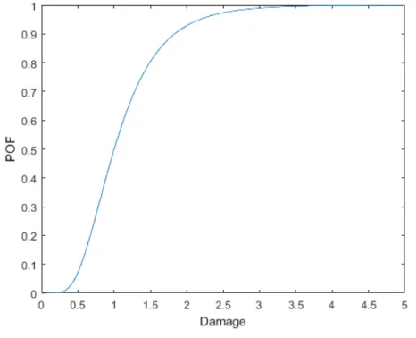
When damage is found, POF can be obtained. Figure 2-2 represents the probability of failure for a certain damage. However, damage is a cumulative value what means that when you reach a certain damage value you have passed through lower damage values as well, so that the POF is the cumulative density function, plotted in Figure 3-1.

Figure 3-1: POF respect to damage

When introducing uncertainty in the damage, the POF will be calculated as follows:

𝑃𝑂𝐹 𝑃 𝑓 1|𝑋 𝑥 ∙ 𝑃 𝑥 ∙ 𝑑𝑥

Where, P(f=1|X=x) is the POF for a value of damage, and P(x) is the probability density function of the damage.

(26)

18

3.3 P

ROBABILITY DENSITY FUNCTIONS IN UNCERTAINTY ANALYSIS

There are three variables in which uncertainty is going to be analyzed. To do that, probability density functions have to be defined to perform Monte Carlo simulations.

Once probability density functions (PDF) of the variables are defined, the PDF of the damage can be obtained simulating cases and then POF can be calculated.

3.3.1 Natural frequency

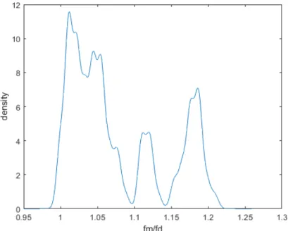
Natural design frequency is usually underestimated compared to the measured one (Kallehave, Byrne, LeBlanc Thilsted, Mikkelsen, & Sciences, 2015). A histogram of the relation between frequencies measured and design can be found in that reference. To consider a smooth probability density function a kernel distribution has been used. Kernel distribution is shown in Figure 3-2.

Figure 3-2: Probability density function of fm/fd

To simulate values of the natural frequency, the cumulative density function (CDF) is obtained summing up the probabilities and dividing into the total probability to normalize. Then, a random value between 0 and 1 is generated and looking in the CDF the “x” that corresponds with that value is obtained.

(27)

19

3.3.2 Damping ratio

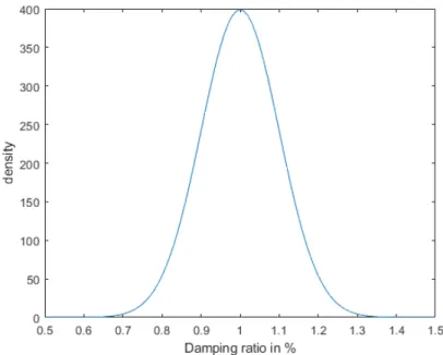
As said before, damping ratio is assumed to be 1% in a normal condition. Change of this value range from 0.8% to 1.2% (Devriendt, Jordaens, De Sitter, & Guillaume, 2013).

The probability density function is assumed to be a normal distribution of 1 % mean value and a 0.1 % standard deviation, so that in two standard deviations (from 0.8 % to 1.2 %) 95% of the cases are included.

Figure 3-3: Probability density function of damping ratio

In this case, for simulating purposes, it is possible to simulate random variables directly from a normal distribution with a known mean and standard deviation.

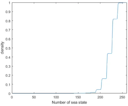
3.3.3 Sea state

In this case, probabilities of each sea state are given in the scatter diagram. To obtain a random sea state the CDF needs to be generated. CDF is created just summing up the probabilities of every sea state to happen and dividing between the total sum to normalize the CDF. Every sea state is given a number considering the order it was summed up to the CDF. A random number between 0 and 1 is generated and then from the CDF a number that corresponds to one of the sea states is obtained. An example of the CDF, it depends on the order you add the sea states, is presented in Figure 3-4.

(28)

20

Figure 3-4: Cumulative density function of sea state

For the simulation of sea states, 3 hours sea states have been used to reduce the number of simulations required, but considering as well that sea states have to remain short enough to assume a stationary process.

(29)

Chapter: Results Daniel Bolado Fernández

21

4 RESULTS

After methodology have been explained POF is obtained for the four design cases: one deterministic approach and three other cases where uncertainty is considered. A discussion is carried out at the same time results are presented.

4.1 D

ESIGN WITHOUT CONSIDERING UNCERTAINTY

A 25 years lifespan of the structure is considered. For the deterministic approach a damage of 0.1581 has been obtained, that leads to a POF of 4.7070∙10-5_{. Normal values obtained for POF at}

fatigue design in industry are around 10-4_{, so this value is a realistic one, and will be used as a}

reference to the rest of the cases where uncertainty is introduced.

4.2 D

ESIGN WITH UNCERTAINTY IN NATURAL FREQUENCY

The POF calculated is 2.4575∙10-5_{, approximately a 54% of the POF when not considering}

uncertainty. Simulation took 1153 s, a relative short time, and considered 1000 different cases.

(30)

22

This reduction in failure probability can be explained once the curve that relates relative frequency and relative damage is found, Figure 4-1. The graph shows that relative damage decreases with increase of the relative frequency. As seen in Chapter 3: Methodology, the frequency values are underestimated so a reduction in damage and POF is expected.

This result could be inferred before performing the simulation knowing than actual frequencies are higher than design values using the following reasoning. For obtaining the damage wave spectrums are used. The design natural frequency is 1.227 rad/s, which correspond to a period of 5.12 s. If frequency is increased the period is lower, which means moving the period further from the wave spectrum peak of the more common waves that have periods of at least 5 s. This reduces the damage and the POF as a consequence. DEL calculation also has a term, ω03/4, that increases damage when

frequency is increased, however the reduction in energy of the waves plays a more important role.

4.3 D

ESIGN WITH UNCERTAINTY IN DAMPING RATIO

In this case, POF obtained is 2.1919∙10-4_{, more than 5 times the POF in the reference case. This}

huge variation in the POF is caused by the large relative interval of damping ratio considered in this project, ± 20% for the 95% of the cases considered. The simulation took 1886 seconds for generating 1000 scenarios, which is an acceptable amount of time.

(31)

23

In the Figure 4-2Figure 4-2, the variation of relative damage respect to the relative variation of damping ratio is shown. The curve observed explain the increase in the POF. It can be seen that lowering damping ratio increases the damage way more than the reduction of damage induced by an increase in damping ratio. So, as the considered probability density function is a normal curve, there are the same probabilities of values being above and below the mean, the damage is expected to increase when considering uncertainty in the damping ratio.

In Figure 4-3, the PDF of the damage is plotted. Commonly, higher values of damage are obtained in comparison with the deterministic damage value, what leads to a higher POF. Effect of random extremely high numbers of damping ratio can cause a significant increase in POF as well.

Figure 4-3: PDF of relative damage with damping ratio uncertainty

4.4 D

ESIGN WITH UNCERTAINTY IN SEA STATES

The POF in this case is obtained depending on the number of iterations of sea states combinations performed during the service time of the structure. 73,000 sea states are included per simulation. The spent time per simulation is 707 s, and total time simulation is 21371 s, for 30 simulations, a relatively long time, but short enough to make Monte Carlo method an acceptable option to simulate the POF in this case.

(32)

24

In Figure 4-4, the relative POF respect to the number of iterations can be found. It can be seen that the relative POF fluctuates rapidly when having few simulations and stabilize when having more than 20 simulations.

Figure 4-4: Relative POF respect to number of simulations

Values of POF range in between a 4% increment and a 3% decrease respect to the reference value. The most extreme variations are found at few iterations where randomness play a huge role. In the Figure 4-5, the PDF of the relative damage respect to the number of iterations is represented. It is seen that the PDF converges when the number of iterations is increased.

(33)

Chapter: Conclusion Daniel Bolado Fernández

25

5 CONCLUSION

This project confirms that Monte Carlo method can be used for including uncertainty in the fatigue design of offshore wind turbine monopile structures, considering the results obtained and also the amount of time spent for simulating.

The POF varies largely with the inclusion of uncertainty, so that uncertainty needs to be considered in design. Following conclusions have been obtained:

- Natural frequency uncertainty produces a lower POF of the structure, so it is not important for the failure of the structure, but it should be considered if a more efficient design of the structure has to be carried out, reducing the costs.

- The variation of damping ratio plays a huge role in the POF as damage dramatically increases when reducing the damping ratio. A bad estimation of this parameter can lead to an unsafe design, so quite much effort should be put in obtaining the possible damping ratio values.

- Eventually, it can be stated that there is not a big difference in results when using a scatter diagram or simulating the actual sea states during the lifespan of the structure.

(34)

Chapter: Conclusion Daniel Bolado Fernández

(35)

References Daniel Bolado Fernández

27

R

EFERENCES

Ansys guide. Modal analysis. Retrieved from http://www.ansys.stuba.sk/html/guide_55/g-str/GSTR3.htm

Barltrop, N. (1991). Dynamics of fixed marine structure. Oxford. In: Butterworth-Heinemann. Cangas, G. (2017). Cálculo Dinámico. Apuntes del M. I.C.C.P. In.

Devriendt, C., Jordaens, P. J., De Sitter, G., & Guillaume, P. J. I. r. p. g. (2013). Damping estimation of an offshore wind turbine on a monopile foundation. 7(4), 401-412.

European Wind Energy Association. (2011). Wind in our sails. The coming of Europe's offshore wind energy industry. Retrieved from

http://www.ewea.org/fileadmin/files/library/publications/reports/Offshore_Report.pdf

Hapel, K.-H. (2013). Festigkeitsanalyse dynamisch beanspruchter offshore-konstruktionen: Springer-Verlag.

Jonkman, J., Butterfield, S., Musial, W., & Scott, G. J. N. R. E. L., Golden, CO, Technical Report No. NREL/TP-500-38060. (2009). Definition of a 5-MW reference wind turbine for offshore system development.

Kallehave, D., Byrne, B. W., LeBlanc Thilsted, C., Mikkelsen, K. K. J. P. T. o. t. R. S. A. M., Physical, & Sciences, E. (2015). Optimization of monopiles for offshore wind turbines.

373(2035), 20140100.

Melchers, R. E., & Beck, A. T. (2018). Structural reliability analysis and prediction: John Wiley & Sons.

Musial, W., & Butterfield, S. (2004). Future for offshore wind energy in the United States. Paper presented at the EnergyOcean 2004 Conference.

Muskulus, M., & Schafhirt, S. (2015). Reliability-based design of wind turbine support

structures. Paper presented at the Proceedings of the Symposium on Reliability of

Engineering System, Hangzhou, China.

OpenCourseWare, M. Percentage of gradient wind velocity. In.

Real, L., Sierra, E., & Almena, A. (2016). Renewable Energy Sector. In Alternative Energy

Sources and Technologies (pp. 17-30): Springer.

Ritchie, H., & Roser, M. (2018). Renewables. Retrieved from

https://ourworldindata.org/renewables

Seidel, M. J. S. (2014). Wave induced fatigue loads: Insights from frequency domain calculations. 83(8), 535-541.

Sørensen, J. N. J. A. R. o. F. M. (2011). Aerodynamic aspects of wind energy conversion. 43, 427-448.

Technica, C. (2017). New Global Offshore Wind Capacity In 2017 Hits 3.3 Gigawatts. Retrieved from https://cleantechnica.com/2018/02/07/new-global-offshore-wind-capacity-2017-hits-3-3-gw/

(36)

References Daniel Bolado Fernández

28

TelosNet. Ilustrated history of wind power development. Retrieved from

http://www.telosnet.com/wind/early.html

U.S. Army Engineer Waterways Experiment Station. (1985). Direct methods for calculating wavelength. Retrieved from

http://acwc.sdp.sirsi.net/client/en_US/default/index.assetbox.assetactionicon.view/104205 8?rm=TECHNICAL+NOTE0%7C%7C%7C1%7C%7C%7C0%7C%7C%7Ctrue

U.S. Energy Information Administration. (2018). History of Wind Power. Retrieved from

https://www.eia.gov/energyexplained/index.php?page=wind_history

Van Der Tempel, J. (2006). Design of support structures for offshore wind turbines. Veritas, D. N. J. D. R. P. D.-R.-C. (2010). Fatigue design of offshore steel structures. Vidal, C. (2017). Modelos espectrales. Apuntes del M. I.C.C.P. In.

Vorpahl, F., Schwarze, H., Fischer, T., Seidel, M., Jonkman, J. J. W. I. R. E., & Environment. (2013). Offshore wind turbine environment, loads, simulation, and design. 2(5), 548-570. Weibull. Miner’s Rule and Cumulative Damage Models. Retrieved from

https://www.weibull.com/hotwire/issue116/hottopics116.htm

World Energy Council. (2016a). Energy resources. Europe. Wind. Retrieved from

https://www.worldenergy.org/data/resources/region/europe/wind/

World Energy Council. (2016b). Energy resources. Wind. Retrieved from

(37)

APPENDIX: MATLAB APPENDIX Daniel Bolado Fernández

29

APPENDIX

MATLAB APPENDIX

In this appendix all the MATLAB code used for obtaining the results of the project is included. The code consists of 4 scripts that calculate the results necessary for the project. Every design approximation (deterministic or natural frequency, damping ratio, sea state uncertainty analysis) has one script. Several functions are used for running those scripts and are also included here.

Deterministic program tic clear all close all syms z

%THIS PROGRAM COMPUTES THE PROBABILITY OF FAILURE OF A MONOPILE STRUCTURE %DETERMINISTIC DESIGN

%Declare the variables

d=15; %water depth

fb=10; %freeboard

th=87.6; %tower height

znac=th+fb+d; %height of nacelle respect to the bottom

D=5; %diameter of the monopile

t=30; %averaged thickness of the monopile and tower

m=4; %average fatigue coefficient

lf=25; %lifespan of the structure

eo=0.01; %damping ratio %Calculate Stress at Failure

[Sf]=StressFailure(m,lf,t);

%Calculate First Mode Shape

[phio,wo,Ko,muz,I]=FirstModeShape(eo,znac,D,t);

%Calculate Hydrodynamic Transfer Function

[Hao]=HydrodynamicTransferFunction(wo,d,D,phio);

%HTB=SD of bending moments over SD of nacelle displacements

HTB=double(wo^2*int(phio*muz*z,0,znac));

%Obtain the wave data from the .txt file

[Tp,Hs,Prob]=ReadData ('wave_data.txt');

%Define variables for iteration

(38)

APPENDIX: MATLAB APPENDIX Daniel Bolado Fernández 30 sDELp=0; sp=0; for i=1:size(Prob,1) for j=1:size(Prob,2) if (Prob(i,j)==0) continue; end

%Obtain Wave Spectrum

[Suuwo]=WaveSpectrum(wo,Tp(j),Hs(i)); %DEL DEL(i,j)=double(1.8825*sqrt(Suuwo)*phio(znac)/Ko*sqrt(1/eo)*wo^(3/4)*Hao*HTB); %Compute probabilities sDELp=sDELp+DEL(i,j)^m*Prob(i,j); sp=sp+Prob(i,j); end end

%Ponderate DEL taking into account Probabilities

DELeq=(sDELp/sp)^(1/m);

%Convert Moments to stress range in MPa

Seq=double(DELeq*2*(D/2)/I)/10^6;

%Damage

Damage=(Seq/Sf)^(m);

%Probability of failure (using failure curve)

muPOF=log(1);

sigmaPOF=sqrt(log(0.5^2+1));

POF=logncdf(Damage,muPOF,sigmaPOF)

toc

Natural frequency uncertainty

tic

clear all

close all

syms z

%THIS PROGRAM COMPUTES THE PROBABILITY OF FAILURE OF A MONOPILE STRUCTURE %TAKING INTO ACCOUNT UNCERTAINTY IN THE FREQUENCY

(39)

31

d=15; %water depth

fb=10; %freeboard

eo=0.01; %damping ratio %Calculate Stress at Failure

%Obtain CDF: Relation between Measured Frequency and Design Frequency

[fmfdcdf,xfmfd]=RelationFMeasuredFDesignCDF;

DEL=zeros(size(Prob)); sDELp=0; sp=0; Damage=zeros(1000,1); RandWm=zeros(1000,1);

for l=1:1000%same number of size of Damage and RandWm

sDELp=0; sp=0; R=rand;

fmfdrnd=xfmfd(find(fmfdcdf>R,1));

wm=wo*fmfdrnd; %Random measured frequency

RandWm(l)=fmfdrnd;

%Calculate Hydodynamic Transfer Function

[Hao]=HydrodynamicTransferFunction(wm,d,D,phio);

HTB=double(wm^2*int(phio*muz*z,0,znac)); for i=1:size(Prob,1) for j=1:size(Prob,2) if (Prob(i,j)==0) continue; end

(40)

APPENDIX: MATLAB APPENDIX Daniel Bolado Fernández 32 %DEL DEL(i,j)=double(1.8825*sqrt(Suuwo)*phio(znac)/Ko*sqrt(1/eo)*wm^(3/4)*Hao*HTB); %Compute probabilities sDELp=sDELp+DEL(i,j)^m*Prob(i,j); sp=sp+Prob(i,j); end end

%Convert Moments to stress in MPa

Seq=double(DELeq*2*(D/2)/I)/10^6; %Damage Damage(l)=(Seq/Sf)^(m); end

%Relation between increase in w and Damage

[RandWm,RandWmsort]=sort(RandWm); %Get the order of Wm and sort

Damage=Damage(RandWmsort);

[POF]=POFIntersection(Damage,0.005);

toc

Damping ratio uncertainty

tic

clear all

close all

syms z

%THIS PROGRAM COMPUTES THE PROBABILITY OF FAILURE OF A MONOPILE STRUCTURE %TAKING INTO ACCOUNT UNCERTAINTY IN THE DAMPING RATIO

d=15; %water depth

fb=10; %freeboard

(41)

33

%Calculate Stress at Failure

%Normal distribution of eo %normpdf(x,0.01,0.001);

DEL=zeros(size(Prob)); sDELp=0; sp=0; Damage=zeros(1000,1); Randeo=zeros(1000,1);

for l=1:1000%same number of size of Damage and Randeo

sDELp=0; sp=0;

eo=normrnd(0.01,0.001); Randeo(l)=eo;

[Hao]=HydrodynamicTransferFunction(wo,d,D,phio);

HTB=double(wo^2*int(phio*muz*z,0,znac)); for i=1:size(Prob,1) for j=1:size(Prob,2) if (Prob(i,j)==0) continue; end

[Suuwo]=WaveSpectrum(wo,Tp(j),Hs(i)); %DEL DEL(i,j)=double(1.8825*sqrt(Suuwo)*phio(znac)/Ko*sqrt(1/eo)*wo^(3/4)*Hao*HTB); %Compute probabilities sDELp=sDELp+DEL(i,j)^m*Prob(i,j); sp=sp+Prob(i,j); end end

(42)

34

Seq=double(DELeq*2*(D/2)/I)/10^6; %Damage Damage(l)=(Seq/Sf)^(m); end toc

%Relation between increase in w and Damage

[Randeo,Randeosort]=sort(Randeo); %Get the order of B

Damage=Damage(Randeosort);

%plot(Randeo,Damage)

[POF]=POFIntersection(Damage,0.005);

toc

Sea state uncertainty

tic

clear all

close all

syms z

%THIS PROGRAM COMPUTES THE PROBABILITY OF FAILURE OF A MONOPILE STRUCTURE %TAKING INTO ACCOUNT UNCERTAINTY IN THE SEA STATE SCATTER DIAGRAM

d=15; %water depth

fb=10; %freeboard

eo=0.01; %damping ratio

NSS=lf*24*365/3; %number of sea states in the lifespan %Calculate Stress at Failure

(43)

35

HTB=double(wo^2*int(phio*muz*z,0,znac));

[Tp,Hs,Prob]=ReadData ('wave_data.txt'); Prob=Prob';

Prob=Prob(:);

DEL=zeros(NSS,1); sDELp=0;

Damage=zeros(30,1); Time=zeros(30,1);

for i=1:30%number of simulations, same as Damage

sDELp=0;

for j=1:NSS

%Obtain Hs and Tp for a random sea state

[HsRand,TpRand]=RandSeaState(Hs,Tp,Prob);

[Suuwo]=WaveSpectrum(wo,TpRand,HsRand); %DEL DEL(j)=double(1.8825*sqrt(Suuwo)*phio(znac)/Ko*sqrt(1/eo)*wo^(3/4)*Hao*HTB); %Compute probabilities sDELp=sDELp+DEL(j)^m; end

DELeq=(sDELp/NSS)^(1/m);

Seq=double(DELeq*2*(D/2)/I)/10^6; %Damage Damage(i)=(Seq/Sf)^(m); Time(i)=toc; end POF=zeros(30,1); for i=1:30

%Probability of failure (using failure curve)

(44)

APPENDIX: MATLAB APPENDIX Daniel Bolado Fernández 36 end Auxiliary functions function [phio,wo,Ko,muz,I]=FirstModeShape(eo,znac,D,t)

syms phio(z) d2phio(z);

gmat=78000; %specific weight (N/m³)

mnac=314520; %mass of the blades+hub+nacelle

g=9.81; %gravity

dint=D-2*t/1000; %int diameter of the monopile

E=2*10^11; %Young's Modulus

I=pi()*(D^4-dint^4)/64; %inertia of a hollow tube

muz=gmat*(D^2-dint^2)*pi()/(4*g); %mass per length

phio(z)=1-cos(pi()*z/(2*znac)); d2phio(z)=diff(phio(z),z,2); Mo=int(muz*phio(z)^2,0,znac)+mnac*phio(znac); Ko=double(int(E*I*d2phio(z)^2,0,znac)); wo=double(sqrt(Ko/Mo)*sqrt(1-eo^2)); end function [Hao]=HydrodynamicTransferFunction(wo,d,D,phio) syms no(z) p=1000; %water density g=9.81; %gravity G=(2*pi()/(2*pi()/wo))^2*d/g; F=G+1/(1.0+0.6522*G+0.4622*G^2+0.0864*G^4+0.0675*G^5);

Lo=(2*pi()/wo)*sqrt(g*d/F);%this value is wave length for mode 0

CM=-2.5*(D/Lo)^3+7.53*(D/Lo)^2-7.9*(D/Lo)+3.2;

if(CM>2) %modify if there is a D(z) not constant

CM=2; end ko=2*pi()/Lo; no(z)=cosh(ko*(z+d))/sinh(ko*d); Hao=double(p*wo^2*int(CM*(pi()*D^2/4)*no(z)*phio,-d,0)); end function [POF]=POFIntersection(Damage,Bw)

%adjust the damage to a kernel distribution

[yf,xf]=ksdensity(Damage,'Bandwidth',Bw); plot(xf/0.1581,yf)

%curve of failure as described in the project

muPOF=log(1);

sigmaPOF=sqrt(log(0.5^2+1));

POFfn=logncdf(xf,muPOF,sigmaPOF);

%P(x)*P(f=1|X=x)

(45)

APPENDIX: MATLAB APPENDIX Daniel Bolado Fernández 37 for i=1:length(xf) y_d(i)=POFfn(i)*yf(i); end %POF POF=trapz(xf,y_d); end function [HsRand,TpRand]=RandSeaState(Hs,Tp,Prob) ycum=cumsum(Prob); ycum=ycum/max(cumsum(Prob));

%simulate random values

R=rand; seastate=find(ycum>R,1); HsRand=Hs(ceil(seastate/length(Tp))); if ((seastate-floor(seastate/length(Tp))*length(Tp))==0) TpRand=Tp(length(Tp)); else TpRand=Tp(seastate-floor(seastate/length(Tp))*length(Tp)); end end function [Tp,Hs,Prob]=ReadData(n) d=dlmread(n,'\t',1,0); Tp=d(1,2:end); Hs=d(2:end,1); Prob=d(2:end,2:end); end function [fmfdcdf,xfmfd]=RelationFMeasuredFDesignCDF

%read data of relation first tower bending frequency measured and designed

fmfd=dlmread('Relation_fmean_fd.txt');

xfmfd=(min(fmfd)-0.05:0.001:max(fmfd)+0.05);

%data adjusted to a kernel distribution

[fmfd,xfmfd] = ksdensity(fmfd,xfmfd,'Bandwidth',0.005); %cdf(xfmfd,fmfd); fmfdcdf=cumsum(fmfd)/max(cumsum(fmfd)); end function [Sf]=StressFailure(m,lf,t)

loga2=12.18; %Table 2-3 DNVGL-RP-C203, tubular joints

tref=16; %(2.4.3) DNVGL-RP-C203, tubular joints

k=0.25; %Thickness exponent

N=lf*365*24*3600;

(46)

APPENDIX: MATLAB APPENDIX Daniel Bolado Fernández 38 end function [Suuwo]=WaveSpectrum(wo,Tp,Hs) sig=0.07; if (wo>(2*pi()/Tp)) sig=0.09; end

gamma=1;%fatigue value

Bj=(0.0624*(1.094-0.01915*log(gamma)))/(0.230+0.0336*gamma-0.185*(1.9+gamma)^(-1)); Suuwo=Bj*Hs^2*Tp^(-4)*(wo/(2*pi()))^(-5)*exp(-1.25*(Tp*(wo/(2*pi())))^(-4))*gamma^(exp(-(Tp*(wo/(2*pi()))-1)^2/(2*sig^2))); end

(47)