Proceedings 2017, 1, 146; doi:10.3390/ecas2017-04147 www.mdpi.com/journal/proceedings Proceedings
Trend Assessment for a CO
2and CH
4Data Series in
Northern Spain
†Beatriz Fernández-Duque *, Isidro A. Pérez, M. Ángeles García, Nuria Pardo and M. Luisa Sánchez
Department of Applied Physics, Faculty of Sciences, University of Valladolid, Paseo de Belén, 7, 47011 Valladolid, Spain; [email protected] (I.A.P.); [email protected] (M.Á.G.);
[email protected] (N.P.); [email protected] (M.L.S.)
* Correspondence: [email protected]; Tel.: +34-983-424-187
† Presented at the 2nd International Electronic Conference on Atmospheric Sciences, 16–31 July 2017; Available online: http://sciforum.net/conference/ecas2017.
Published: 17 July 2017
Abstract: The main objective of this paper is to implement different methods to assess the salient features of the data trend for a CO2 and CH4 data series. Said series was obtained at the Low
Atmosphere Research Centre (41°48′49″ N, 4°55′59″ W) using a Picarro analyser (G1301). Different functions were employed to determine and quantify the data trend. The first was a harmonic function based on a third-degree polynomial. An increasing trend, below 2.30 ppm year−1 for CO2
and below 11.90 ppb year−1 for CH4, was reported. Epanechnikov, Gaussian, biweight, tricubic,
rectangular and triangle kernels, were applied with a 500-day bandwidth for the trend. The best fit was obtained by the biweight kernel (r > 0.20), with an increasing trend around 1.80 ppm year−1 for
CO2 and around 7.15 ppb year−1 for CH4. The final analysis, which included local linear regression
functions also applying a 500-day bandwidth, revealed increasing trends for both CO2, around 1.98
ppm year−1, and CH4, around 10.85 ppb year−1. Trend values were far more accelerated in the latter
years of the series, regardless of the chosen function. This paper demonstrated the usefulness of the mathematical functions, allowing for an accurate determination of the data trend.
Keywords: trend; harmonic function; kernel functions; local linear regressions; daytime; night-time
1. Introduction
CO2 and CH4 have been the focus of intensive research at different sites in an effort to gain
insights into their evolution, given their link to climate change [1]. Small changes in the trends of greenhouse gases can have a major impact on the Earth, and thus may be of great significance for climate change [2].
The decomposition of an atmospheric time series into its constituent parts is essential for identifying and isolating variations of interest from a data set, and is widely used to obtain information about sources, sinks and trends in climatically important gases. An atmospheric data record is the result of a long-term trend, a short term and a random term resulting from anomalous observations. Due to the periodic and irregular variations on both long and short timescales, analysis of atmospheric time series is a complex process. The long-term is mainly derived from fossil fuel burning processes and from land-use change emissions, overlapped to a large interannual variability related to climate-driven changes in source and sinks [2,3]. Studying the data trend requires subtracting the seasonal component from the complete time series by a deseasonalization process. This procedure involves fitting appropriate mathematical functions to the data [2].
pollution analysis. Cleveland [7] suggested local regression methods to obtain visual information from scatterplots [8]. Kernel smoothing functions are an extension of the locally weighted average method which has been widely used in atmospheric temporal series [9]. Moreover, kernel regression methods have successfully been used in different air pollution data. According to de Haan [10], Lorimer was the first author to use the kernel method for atmospheric dispersion modelling of inert airborne contaminants [11]. Since then, many authors have employed this mathematical technique to atmospheric time series [9,12].
Thus, the main goal of the current study is to quantify the trend evolution of a CO2 and CH4 data
series by applying harmonic functions, kernel techniques and, finally, local linear functions. The results may be helpful as regards improving our understanding of the temporal evolution of both gases in a Mediterranean rural area of northern Spain.
2. Data and Methods
2.1. Data Acquisition and Calibration
The measuring campaign took place from mid October 2010 to late February 2016, and consisted of 30-min mixing ratio averages. Semi-hourly measurements were divided into diurnal and nocturnal records. Measurements were carried out at the Low Atmosphere Research Centre, CIBA station (41°48′49″ N, 4°55′59″ W) with a Picarro G1301 analyser, which is based on cavity ring-down spectroscopy. A detailed explanation of this technique is given in [13,14].
The analyser is equipped with three external solenoid valves which measure at a height of 1.8, 3.7 and 8.3 m. Only the highest level was considered in the current paper. Values provided by the device were slightly corrected by using linear equations obtained with calibrations performed fortnightly with three NOAA calibration gas standards. The following equations, taken from Pérez et al. [1] (in ppm), were applied to the data to correct the measurements obtained with the analyser:
CO = 1.00341 CO − 0.17870 (1)
CH = 0.99197 CH + 0.01249 (2)
where C means the corrected value.
2.2. Site Location
The sampling area is located in a semi-natural area over an extensive plateau 845 m above sea level in northern Spain. Located 24 and 40 km from two of the region’s main cities, and with no major roads nearby, the station was able to provide essential information on CO2 and CH4 sources and sinks
within the Spanish upper plateau (Figure 1).
Agricultural crops, Mediterranean shrubs and stands of coniferous trees make up the surrounding vegetation. The site is classed as Mediterranean North, with maximum precipitation in autumn and spring and minimum during the summer season [15,16] (Figure 2).
Figure 2. PNOA image courtesy of ©ign.es, showing the main vegetation ecosystems around the monitoring station, which is surrounded by a black line.
2.3. Mathematical Procedure
2.3.1. Harmonic Function
The harmonic function employed (Equation (3)) is based on the equation proposed by Fernández-Duque et al. [6]. In this study, the authors analysed the temporal evolution for a CO2 and
CH4 data set with a harmonic function comprising a third-degree polynomial term which expresses
the data trend and a series of four harmonics which reflect seasonality. The equation used is described below:
= ∑ + ∑ ∑ t cos 2 + t sin 2 (3)
where y expresses the mixing ratio in ppm for CO2 and ppb for CH4, whereas time (t) is expressed in
years. The four harmonics involved in the equation consider the amplitude as a fixed (k = 0) and variable (k = 1) term over time in order to obtain more accurate results. The unknown coefficients of the multiple harmonic regression were obtained using MATLAB © software.
2.3.2. Kernel Function
The average smoothed mixing ratios employing the kernel procedure can be obtained by using Equation (4):
, ℎ =∑
∑ (4)
where t refers to time expressed in years, h is the smoothing parameter expressed in days, N is the number of data, K is the kernel function employed, and yi is the mixing ratio in a time ti. Six different
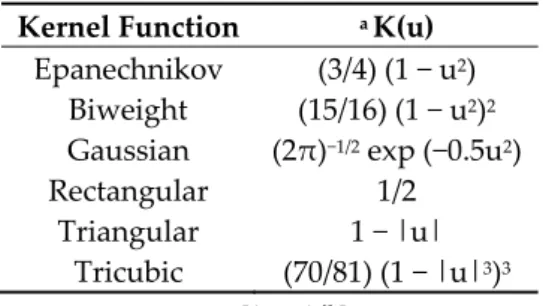
Table 1. Kernel functions employed in the study.
Kernel Function a K(u)
Epanechnikov (3/4) (1 − u2)
Biweight (15/16) (1 − u2)2
Gaussian (2π)−1/2 exp (−0.5u2)
Rectangular 1/2 Triangular 1 − |u|
Tricubic (70/81) (1 − |u|3)3 a u = [(t−ti)/h].
It should be taken into account that the u value for which k(u) > 0 takes positive values ranges between −1 and 1, except for the Gaussian kernel which comprises the whole real line. Each of the kernels employed in the smoothing process is centred as its respective data value ti and is scaled in
width relative to the shapes by the smoothing parameter h. If the h value is small, great weight is attached to the neighbouring observations, resulting in a rough estimation. On the other hand, a large h value may lead to significant smoothing, masking the behaviour at certain scales [17]. In order to avoid oscillations, the use of high smoothing factors is recommended even though some peak locations may be lost. A 500-day bandwidth for expressing the trend was used.
2.3.3. Local Linear Function
The second non-parametric technique employed in this paper was the weighted local linear regression function, which may be stated as follows:
y = a0+a1t (5)
where a0 and a1 were calculated according to expressions (6) and (7):
=∑ − −
∑ − (6)
= − (7)
where wi are the weights and and are weighted mean values, calculated according to the
procedure described by Pérez et al. [8]. It should be considered that in this case, the Epanechnikov kernel was used, since it is the most widely used kernel in atmospheric studies and also because of its simplicity. A 500-day bandwidth for expressing the trend was also used for this analysis.
3. Results and Discussion
3.1. CO2 and CH4 Mixing Ratio Evolution
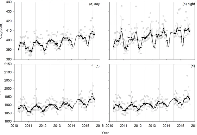
Figure 3 reflects the evolution of both gases. Middle black solid dots correspond to the monthly median values, and while lines correspond to the interquartile range. The upper open and grey dots represent the 90th percentile while the lower ones denote the 10th percentile. Finally, the solid black lines show the data trend evolution, which was calculated using the harmonic function (Equation (1)). Figure 3a,b shows the variability of average CO2 mixing ratios over time. CO2 evolution presents
a maximum in the winter season, followed by another maximum in spring which is only detectable for nocturnal records. The winter peak is mainly related with local emissions from vehicles, industrial activities and domestic heating, as suggested García et al. [16]. The spring maximum at nights is related with strong temperature inversions at the sampling site, which contribute to trapping CO2
Figure 3. CO2 and CH4 evolution during the whole study period at CIBA station. (a,b) represent CO2 diurnal and nocturnal results, respectively, while (c,d) correspond to CH4 diurnal and nocturnal results respectively.
The CH4 cycle (Figure 3c,d) is less pronounced than the CO2 cycle, although differences between
day and night could also be inferred. Higher values were detected at nights due to lower planetary boundary layer heights which inhibit vertical mixing movements. 90th percentile values, which are around 1.95 ppb, might be attributed to fugitive emissions from an urban landfill near the sampling site and from high emissions from the nearby cities as pointed out by Sánchez et al. [18]. The main statistics for the CO2 and CH4 mixing ratios at the CIBA station are presented in Table 2.
Table 2. Monthly means statistics of the measured CO2 and CH4 mixing ratios.
Statistic CO2(ppm) CH4(ppb)
Day Night Day Night
Median 397.91 403.24 1.8966 1.9024 Interquartile range 5.01 7.98 0.0284 0.0315
10th percentile 394.34 397.87 1.8737 1.8772 90th percentile 405.72 414.74 1.9368 1.9446
All the statistics studied (Table 2) display higher values for nocturnal records. The different behaviour between day and night is in line with a lower development of the mixing layer height together with greater emissions from vehicles at night leading to higher mixing ratio values. In contrast, more intense solar radiation during the daytime produces an increase in the mixing layer height and, therefore, efficient dilution of gases from surface decreasing mixing ratio measures [16].
Had we considered the whole data set without differentiating day measurements from night measurements, the main CO2 statistics presented in Table 2 would be consistent with those presented
3.2. Data Trend Evolution
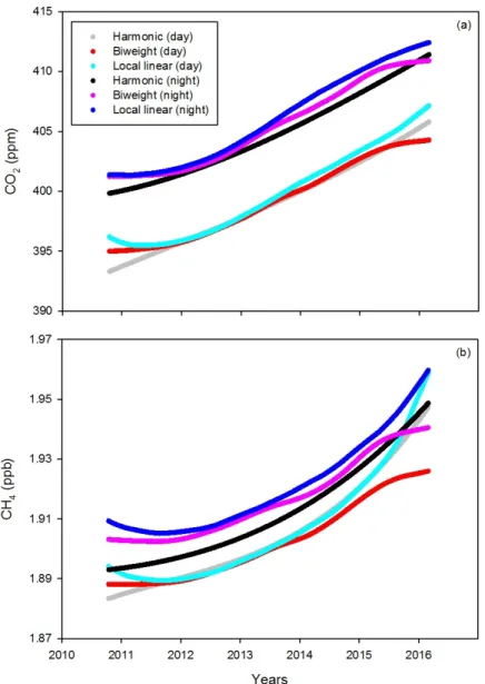
Figure 4 reflects the CO2 and CH4 trend evolution by using the three different mathematical
functions described in Section 2.3. As regards harmonic functions, only the polynomial term was employed in this section since this is the term that expresses the data trend.
Six different kernel functions, listed in Table 1, were used to obtain the CO2 and CH4 trend.
However, only the biweight kernel is presented in Figure 4 since this function provides the best fit for both the CO2(r > 0.40) and CH4(r > 0.20) dataset. As regards the local weighted method, the
Epanechnikov kernel was employed because of its simplicity and low computational effort, since only a fraction of the observations in the neighbourhood of the calculation points were considered. In both cases, a 500-day bandwidth was applied to the dataset. We found that trend curves fit the experimental data provided by the Picarro (G1301) analyser well, showing few differences among the three mathematical functions.
Figure 4. CO2 and CH4 multi-year observed trend plotted as semi-hourly mixing ratio averages. (a) CO2 results; (b) CH4 results.
A well-defined increasing pattern over the years was inferred from Figure 4, which is partially related with a rise in anthropogenic emissions from industrial activities and from the urban landfill near the monitoring station for CH4, as well as from farming vehicle emissions [8]. The same
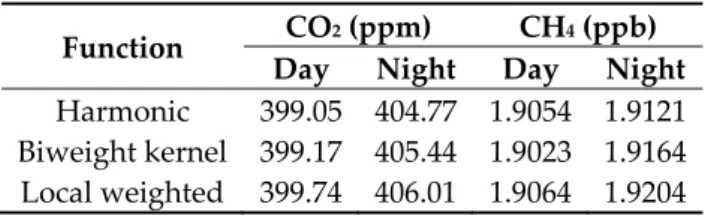
Table 3 gives a summary of the mean trend values by using the different functions. Higher nocturnal than diurnal values for both CO2 and CH4 were found mainly as a result of the evolution
of the boundary layer, biological processes and the influence of industrial emissions.
Table 3. Mean trend values for CO2 and CH4 by applying the three mathematical functions.
Function CO2(ppm) CH4(ppb)
Day Night Day Night
Harmonic 399.05 404.77 1.9054 1.9121 Biweight kernel 399.17 405.44 1.9023 1.9164 Local weighted 399.74 406.01 1.9064 1.9204
Mean CO2 growth values reported for the study area were approximately 2 ppm year−1 for the
three mathematical functions. Specifically, a positive trend below 2.30 ppm year−1 for CO2 and below
11.90 ppb year−1 for CH4 was detected by employing harmonic functions. Similar values were found
with the local linear regression functions, reaching 1.98 ppm year−1 for CO2 and around 10.85 ppb
year−1 for CH4. As regards the kernel functions, slightly lower values were recorded for CO2, around
1.80 ppm year−1, while for CH4 the mean growth rate yielded 7.15 ppb year−1. In all cases, mean trend
values were far more accelerated in the latter years, which might be the result of a rise in emissions of both gases due to industrial activities. These mean trend values were in agreement with those found by Zhang et al. and Zhu et al. [19,20], which were in the range of 1.7–3.6 ppm year−1 for CO2,
and with the results reported by several authors [21–23], which were in the range of 6–10 ppb year−1
for CH4.
Harmonic functions lead to greater values and smoother trend curves since all the data observations contribute to the calculations, while kernel and local weighted functions only consider a narrow interval calculation, ranging between −1 and 1. Furthermore, the border effect of kernel and local functions causes less smooth graphical outputs at the start and end of the series.
4. Conclusions
This paper presents the results of the data trend evolution for a CO2 and CH4 data series by using
harmonic, kernel and local linear functions at the CIBA station. We have also investigated the influence of six different kernel functions when estimating the data trend applying the kernel procedure. We failed to find any major differences between the kernels, although slightly better fits were obtained with the biweight kernel. For this reason, only the biweight kernel is presented in the present study. Our comparisons between functions showed no major differences between the outputs, and report very similar trends for both CO2 and CH4. Thus, we can conclude that harmonic functions,
Kernel functions and local weighted functions were found to be effective methods of describing the CO2 and CH4 data trend in this Mediterranean rural area of northern Spain. These mathematical
functions described the behaviour at the site, producing meaningful information for air quality modelling of both important greenhouse gases in the lower atmosphere.
Acknowledgments: The authors of this paper acknowledge financial support from the Spanish Ministry of Economy and Competitiveness and ERDF funds (projects CGL2009-11979 and CGL2014-53948-P).
Author Contributions: Beatriz Fernández-Duque; Isidro A. Pérez and M. Luisa Sánchez conceived and designed the experiments; Beatriz Fernández-Duque performed the data analysis, interpreted the data and wrote this contribution; Isidro A. Pérez and M. Luisa Sánchez supervised the data analysis and the interpretations of the results; M. Ángeles García and Nuria Pardo carried out the calibrations, maintenance of equipment and data processing.
References
1. Pérez, I.A.; Sánchez, M.L.; García, M.Á.; Pardo, N. Carbon dioxide at an unpolluted site analysed with the smoothing kernel method and skewed distributions. Sci. Total Environ. 2013, 456, 239–245, doi:10.1016/j.scitotenv.2013.03.075.
2. Pickers, P.A.; Manning, A.C. Investigating bias in the application of curve fitting programs to atmospheric time series. Atmos. Meas. Tech. 2015, 8, 1469–1489, doi:10.5194/amt-8-1469-2015.
3. Artuso, F.; Chamard, P.; Piacentino, S.; Sferlazzo, D.M.; De Silvestri, L.; di Sarra, A.; Meloni, D.; Monteleone, F. Influence of transport and trends in atmospheric CO2 at Lampedusa. Atmos. Environ. 2009, 43, 3044–3051, doi:10.1016/j.atmosenv.2009.03.027.
4. Anderson-Cook, C.M. A second order model for cylindrical data. J. Stat. Comput. Simul. 2000, 66, 51–65. 5. Sánchez, M.L.; Pérez, I.A.; García, M.A. Study of CO2 variability at different temporal scales recorded in a
rural Spanish site. Agric. For. Meteorol. 2010, 150, 1168–1173, doi:10.1016/j.agrformet.2010.04.018.
6. Fernández-Duque, B.; Pérez, I.A.; Sánchez, M.L.; García, M.Á.; Pardo, N. Temporal patterns of CO2 and CH4 in a rural area in northern Spain described by a harmonic equation over 2010–2016. Sci. Total. Environ.
2017, 593, 1–9, doi:10.1016/j.scitotenv.2017.03.132.
7. Cleveland, W.S. Robust locally weighted regression and smoothing scatterplots. J. Am. Stat. Assoc. 1979, 74, 829–836, doi:10.1080/01621459.1979.10481038.
8. Pérez, I.A.; Sánchez, M.L.; García, M.Á.; Pardo, N. Trend analysis of CO2 and CH4 recorded at a semi-natural site in the northern plateau of the Iberian Peninsula. Atmos. Environ. 2017, 151, 24–33, doi:10.1016/j.atmosenv.2016.11.068.
9. Pérez, I.A.; Sánchez, M.L.; García, M.Á.; Pardo, N. Daily patterns of CO2 in the lower atmosphere of a rural site. Theor. Appl. Climatol. 2015, 122, 195–205, doi:10.1007/s00704-014-1294-9.
10. De Haan, P. On the use of density kernels for concentration estimations within particle and puff dispersion models. Atmos. Environ. 1999, 33, 2007–2021, doi:10.1016/S1352-2310(98)00424-5.
11. Lorimer, G.S. The Kernel method for air quality modelling-I. Mathematical foundation. Atmos. Environ.
1986, 20, 1447–1452, doi:10.1016/0004-6981(86)90016-8.
12. Donnelly, A.; Broderick, B.; Misstear, B. Relating background NO2 concentrations in air to air mass history using non-parametric regression methods: Application at two background sites in Ireland. Environ. Model. Assess. 2012, 17, 363–373, doi:10.1007/s10666-011-9301-3.
13. Crosson, E.R. A cavity ring-down analyzer for measuring atmospheric levels of methane, carbon dioxide, and water vapor. Appl. Phys. B 2008, 92, 403–408, doi:10.1007/s00340-008-3135-y.
14. Rella, C.W.; Chen, H.; Andrews, A.E.; Filges, A.; Gerbig, C.; Hatakka, J.; Karion, A.; Miles, N.L.; Richardson, S.J.; Steinbacher, M.; et al. High accuracy measurements of dry mole fractions of carbon dioxide and methane in humid air. Atmos. Meas. Tech. 2013, 6, 837–860, doi:10.5194/amt-6-837-2013.
15. Pérez, I.A.; Sánchez, M.L.; García, M.Á.; Pardo, N. Features of the annual evolution of CO2 and CH4 in the atmosphere of a Mediterranean climate site studied using a nonparametric and a harmonic function. Atmos. Pollut. Res. 2016, 7, 1013–1021, doi:10.1016/j.apr.2016.06.006.
16. García, M.Á.; Sánchez, M.L.; Pérez, I.A. Differences between carbon dioxide levels over suburban and rural sites in Northern Spain. Environ. Sci. Pollut. Res. 2012, 19, 432–439, doi:10.1007/s11356-011-0575-4.
17. Wilks, D.S. Statistical Methods in the Atmospheric Sciences, 2nd ed.; Elsevier: Amsterdam, The Netherlands, 2006; Volume 91, Chapter 3.
18. Sánchez, M.L.; García, M.A.; Pérez, I.A.; Pardo, N. CH4 continuous measurements in the upper Spanish plateau. Environ. Monit. Assess. 2014, 186, 2823–2834, doi:10.1007/s10661-013-3583-7.
19. Zhang, D.; Tang, J.; Shi, G.; Nakazawa, T.; Aoki, S.; Sugawara, S.; Wen, M.; Morimoto, S.; Patra, P.K.; Hayasaka, T.; et al. Temporal and spatial variations of the atmospheric CO2 concentration in China.
Geophys. Res. Lett. 2008, 35, L03801, doi:10.1029/2007GL032531.
20. Zhu, C.; Yoshikawa-Inoue, H. Seven years of observational atmospheric CO2 at a maritime site in northernmost Japan and its implications. Sci. Total Environ. 2015, 524, 331–337, doi:10.1016/j.scitotenv.2015.04.044
21. Fang, S.X.; Tans, P.P.; Dong, F.; Zhou, H.; Luan, T. Characteristics of atmospheric CO2 and CH4 at the Shangdianzi regional background station in China. Atmos. Environ. 2016, 131, 1–8, doi:10.1016/j.atmosenv.2016.01.044.
23. Vermeulen, A.T.; Hensen, A.; Popa, M.E.; van den Bulk, W.C.M.; Jongejan, P.A.C. Greenhouse gas observations from Cabauw Tall Tower (1992–2010). Atmos. Meas. Tech. 2011, 4, 617–644, doi:10.5194/amt-4-617-2011.