A second order in time modified Lagrange-Galerkin finite element method for the incompressible Navier-Stokes equations

(1)

UMER. NAL c

Vol. 50, No. 6, pp. 3084–3109

A SECOND ORDER IN TIME MODIFIED LAGRANGE–GALERKIN

FINITE ELEMENT METHOD FOR THE INCOMPRESSIBLE

NAVIER–STOKES EQUATIONS

∗

R. BERMEJO†, P. GAL ´AN DEL SASTRE†, AND L. SAAVEDRA‡

Dedicated to Professor J. Ildefonso D´ıaz on the occasion of his60th birthday

Abstract. We introduce a second order in time modified Lagrange–Galerkin (MLG) method for the time dependent incompressible Navier–Stokes equations. The main ingredient of the new method is the scheme proposed to calculate in a more efficient manner the Galerkin projection of the functions transported along the characteristic curves of the transport operator. We present error estimates for velocity and pressure in the framework of mixed finite elements when either the mini-element or the

P2/P1 Taylor–Hood element are used.

Key words. Lagrange–Galerkin, Navier–Stokes equations, mixed ﬁnite elements

AMS subject classifications.65M12, 65M25, 65M60

DOI.10.1137/11085548X

1. Introduction.

The Lagrange–Galerkin (LG) method was introduced in the

early 1980s by [6], [17], and [8] (see also [9]) to calculate a numerical solution of time

dependent convection-diﬀusion problems, including the incompressible Navier–Stokes

equations, represented by a diﬀerential equation of the form

Dv

Dt

+

Av

=

f,

where

_DtD

:=

_∂t∂

+

u

· ∇

,

u

being a ﬂow velocity, is the so-called transport operator,

and

A

is a second order elliptic operator modeling the diﬀusion mechanism. The

idea of this method is to combine an implicit backward in time discretization of the

diﬀerential equation, along the characteristic curves of the transport operator, with

a Galerkin projection in the framework of ﬁnite element methods (note that such an

idea is also applicable in the context of spectral methods or hp-ﬁnite element methods;

see, for instance, [19] and [10]), yielding in this way a marching in time procedure

that may be very eﬃcient for the following reasons: (i) the method partially

circum-vents the troubles caused by the convective terms because discretizing backward along

the characteristic curves is a natural way of introducing upwinding in the space

dis-cretization of the diﬀerential equation; (ii) the resulting system of algebraic equations

is symmetric and linear if the operator

A

is also, with a moderate condition

num-ber; (iii) the method is unconditionally stable if the Galerkin projection is performed

exactly; this allows us to use a large time step Δ

t

in the calculations.

Nevertheless, the LG method has several drawbacks: (i) the calculation of the

feet of the characteristic curves at every time step; this requires solving, backward in

∗_{Received by the editors November 16, 2011; accepted for publication (in revised form) August 3,}

2012; published electronically November 29, 2012. This work was supported by the Ministerio de Educaci´on y Ciencia de Espa˜na via grants CGL2007-66440-CO4-01 and ENE2005-09190-C04-01/CON.

http://www.siam.org/journals/sinum/50-6/85548.html

†_{Departamento Matem´}_{atica Aplicada ETSII, Universidad Polit´}_{ecnica de Madrid, 28006 Madrid,}

Spain ([email protected], [email protected]).

‡_{Departamento Fundamentos Matem´}_{aticos ETSIA, Universidad Polit´}_{ecnica de Madrid, 28040}

Madrid, Spain ([email protected]).

3084

(2)

time, many systems of ordinary diﬀerential equations (ODEs); and (ii) the calculation

of some integrals, which come from the Galerkin projection, whose integrands are the

product of functions defined in two different meshes. The first shortcoming is in some

way related to the second because the integrals have to be computed exactly, but in

general it cannot be done this way and they have to be numerically calculated with

high accuracy to keep the method stable; see, in this respect, [2] where a study on

the behavior of the method with diﬀerent quadrature rules is performed. The use of

high order quadrature rules means that many quadrature points per element should

be employed to evaluate the integrals, and, therefore, since each quadrature point has

an associated departure point, many systems of ODEs have to be solved numerically

at every time step; hence, the whole procedure may become less eﬃcient than it looks

at ﬁrst, in particular when working in unstructured meshes, because the numerical

calculation of the feet of the characteristic curves requires locating and identifying of

the elements containing such points, and this task is not easy to do in such meshes.

In [3] we introduced modiﬁed Lagrange–Galerkin (MLG) methods to partly

over-come drawback (ii) of the conventional LG method while maintaining its rate of

convergence when linear or quadratic ﬁnite elements are employed. The goal of this

paper is to describe and analyze the convergence of an MLG method when it is applied

to integrate the time dependent incompressible Navier–Stokes equations; in

particu-lar, we shall study the MLG method combined with the backward diﬀerentiation

formula of order 2 (BDF2) as a time stepping scheme. The LG method combined

with the BDF2 in a ﬁnite element context was presented for the ﬁrst time in [7] to

integrate convection diﬀusion problems; later on, [5] applied this method to integrate

the incompressible Navier–Stokes equations.

We introduce some notation about the functional spaces we use in the paper. For

s

≥

0 real and real 1

≤

p

≤ ∞

,

W

s,p

(

D

) denotes the real Sobolev spaces deﬁned

on

D

for scalar real-valued functions.

·

_Ws,p₍D)

and

|·|

Ws,p₍D)

denote the norm and

seminorm, respectively, of

W

s,p

₍

_D

_{). When}

_s

_{= 0,}

_W

0,p

₍

_D

_{) :=}

_L

p

₍

_D

_{). For}

_p

_{= 2,}

the spaces

W

s,2

₍

_D

_{) are denoted by}

_H

s

₍

_D

_{), which are real Hilbert spaces with inner}

product (

· ,

· )

s

. For

s

= 0,

H

0

(

D

) :=

L

2

(

D

), the inner product in

L

2

(

D

) is denoted by

(

· ,

· ).

H

₀1

(

D

) is the space of functions of

H

1

(

D

) which vanish on the boundary

∂D

in

the sense of trace.

H

−1

denotes the dual of

H

₀1

(

D

). The corresponding spaces of real

vector-valued functions,

v

:

D

→

R

d

_,

_{d >}

_{1 integer, are denoted by boldface letters,}

for instance,

W

s,p

(

D

) := (

W

s,p

(

D

))

d

:=

{

v

:

D

→

R

d

:

v

i

∈

W

s,p

(

D

)

,

1 ≤

i

≤

d

}

.

Let

X

be a real Banach space (

X,

·

_X

). If

v

: (0

, T

)

→

X

is a strongly measurable

function with values in

X

, we set

v

_Lp₍₀,t;X)

= (

t

0

v

(

τ

)

p X

dτ

)

1

/p

_{for 1}

_≤

_{p <}

_∞

_{, and}

v

_L∞₍₀,t;X)

=

ess

sup

0<τ≤t

v

(

τ

)

X

; when

t

=

T

, we shall write, unless otherwise

stated,

v

_Lp₍X)

. We shall also use the following discrete norms:

v

_lp₍X)

=

Δ

t

N

i=1

v

(

τ

i

)

p X

1/p

,

v

_l∞₍X)

= max

1≤i_≤N

v

(

τ

i

)

X

.

Finally, we shall also make use of the space of continuous and bounded functions

in time with values in

X

denoted by

C

([0

, T

];

X

), and the space

C

r,1

(

D

),

r

≥

0, of

functions deﬁned in the closure of D,

r

-times diﬀerentiable and with the

r

th derivative

being Lipschitz continuous.

The layout of the paper is as follows. In section 2 we introduce the continuous

problem and its functional framework. In section 3 we describe the application of the

MLG–BDF2 method to resolve the Navier–Stokes equations, using either the so-called

(3)

3086

R. BERMEJO, P. GAL ´AN DEL SASTRE, AND L. SAAVEDRA

mini-element or

P

₂

/P

₁

Taylor–Hood element. Section 4 is devoted to the numerical

analysis of the method.

2. The continuous problem.

Let

D

⊂

R

d

₍

_d

_{= 2 or 3) be a bounded domain}

with smooth boundary

∂D

, and let [0

, T

] denote a time interval. For further

informa-tion on the regularity hypotheses and the existence and uniqueness of the soluinforma-tions

of the Navier–Stokes equations, see [13] and [20]. In

Q

T

:=

D

×

(0

, T

) we consider

the Navier–Stokes equations for a ﬂuid of constant density

ρ

(for simplicity we take

ρ

= 1) under the action of an external force ﬁeld

f

(

x, t

) and with the known initial

velocity,

u

(

x,

0) =

u

0

(

x

),

(2.1)

∂u

∂t

+ (

u

· ∇

)

u

+

∇

p

−

ν

Δ

u

=

f,

div

u

= 0

, u

|

∂D

= 0

,

where

u

:

D

×

[0

, T

)

→

R

d

_{is the ﬂow velocity,}

_p

_:

_D

_×

₍₀

_{, T}

₎

_→

_R

_{is the}

pres-sure, and

f

:

D

×

(0

, T

)

→

R

d

_{denotes the density of the body forces per unit of}

mass.

ν >

0 is the kinematic viscosity coeﬃcient, which is assumed to be

con-stant. For the mathematical and numerical analysis of the solutions of (2.1) the

following functional spaces are needed:

V

:=

u

∈

H

1₀

(

D

) : div

u

= 0 in

D

,

H

:=

u

∈

L

2

(

D

) : div

u

= 0 in

D

and

n

· u

= 0 on

∂D

, where

n

is the unit outward

nor-mal to

∂D

,

L

2₀

(

D

) :=

q

∈

L

2

(

D

) :

_D

q

= 0

.

. To calculate a numerical solution to

(2.1) we use the following weak formulation [20].

Given

f

∈

L

2

(

H

−1

)

and

u

0

∈

H

, ﬁnd

u

∈

L

2

(

H

1₀

(

D

))

∩

L

∞

(

L

2

(

D

))

and

p

∈

L

2

(

L

2₀

(

D

))

such that for all

v

∈

H

₀1

(

D

)

and

q

∈

L

2₀

(

D

)

,

(2.2)

⎧

⎪

⎨

⎪

⎩

d

dt

(

u, v

) + ((

u

· ∇

)

u, v

) +

ν

(

∇

u,

∇

v

)

−

(

p,

div

v

) = (

f, v

)

,

(div

u, q

) = 0

.

2.1. Semidiscrete BDF2 Lagrangian formulation of the Navier–Stokes

equations.

To motivate the introduction of the MLG–BDF2 method, we present

the BDF2 discretization of the Navier–Stokes equations, backward in time, along the

characteristics of the operator

_DtD

in an interval

I

τ

:= [

τ, s

]

⊂

[0

, T

],

s > τ

. To this

end, we consider the mapping

x

∈

D

→

X

(

x, s

;

t

)

∈

D, t

∈

I

τ

, deﬁned by the initial

value problem

(2.3a)

⎧

⎪

⎨

⎪

⎩

dX

dt

=

u

(

X

(

x, s

;

t

)

, t

)

,

X

(

x, s

;

s

) =

x.

If

u

∈

L

1

(

τ, s

;

W

1,∞

₍

_D

_{)), this problem has a unique solution of the form}

(2.3b)

X

(

x, s

;

t

) =

x

+

t

s

u

(

X

(

x, s

;

τ

)

, τ

)

dτ.

t

→

X

(

x, s

;

t

) is a characteristic curve that represents the trajectory of a ﬂuid particle

that at time

s

will be at

x

. It is worth remarking that the mapping

X

(

x, s

;

t

) has

the group property; i.e., let

t

₁

and

t

₂

∈

I

τ

,

t

1

< t

2

; then

X

(

x, s

;

t

1

) =

X

(

· , t

2

;

t

1

)

◦

X

(

x, s

;

t

₂

). Hereafter, to simplify the writing of the formulas, unless otherwise stated,

we adopt the notation

X

k,l

₍

_x

_{) :=}

_X

₍

_{x, t}

l

;

t

k

),

k

and

l

being positive integers. The

following results, which are needed below, are well known.

(4)

Lemma 2.1.

Assume that

u

∈

L

∞

(

W

1,∞

(

D

))

and

s

−

τ

is suﬃciently small;

then

x

∈

D

→

X

(

x, s

;

t

)

is a quasi-isometric homeomorphism of

D

onto

D

and its

Jacobian determinant

J

= 1

almost everywhere (

a.e.

) in

D

. Moreover,

K

u−1

|

x

−

z

| ≤ |

X

(

x, s

;

τ

)

−

X

(

z, s

;

τ

)

| ≤

K

u

|

x

−

z

|

,

where

K

u

= exp((

s

−

τ

)

∇

u

L∞(0,T;L∞(D))

)

and

|

a

−

b

|

denotes the Euclidean distance

between the points

a

and

b

∈

R

d

.

For a proof of this lemma see [18].

In the following lemma we put together

some facts concerning the solution of (2.3a) which are standard in the theory of ODE

systems.

Lemma 2.2.

Assume that

u

∈

L

∞

(

W

k,∞

(

D

))

, k

≥

1 . Then for any integer

n

,

0 ≤

n

≤

N

−

1 , the unique solution

t

→

X

(

x, t

n+1

;

t

) (

t

∈

[

t

n

, t

n+1

]

⊂

[0

, T

])

of

(2

.

3 a

)

is such that

X

(

x, t

n+1

;

t

)

∈

W

1,∞

(

W

k,∞

(

D

))

. Furthermore, let the multi-index

α

∈

N

d

; then for all

α

such that

1 ≤ |

α

| ≤

k

,

∂

x|αj|

X

i

(

x, t

n+1

;

t

)

∈

C

([0

, T

];

L

∞

(

D

×

[0

, T

]))

,

1 ≤

i, j

≤

d

.

Let 0 =

t

₁

< t

₂

<

· · ·

< t

N

=

T

be a uniform partition of step Δ

t

of the interval

[0

, T

]. For

x

ﬁxed let us consider the diﬀerential equation

dy

(

x, t

)

dt

=

f

(

y, t

)

,

t

∈

(0

, T

];

the BDF2 discretization of this equation at time

t

n₊₁

is of the form

d

t

y

(

x, t

n+1

) =

f

(

y

(

x, t

n+1

)

, t

n+1

)

,

where

d

t

y

(

x, t

n₊₁

) :=

3 y

(

x, t

n₊₁

)

−

4 y

(

x, t

n

) +

y

(

x, t

n₋₁

)

2Δ

t

;

then, noting that

X

n+1,n+1

(

x

) =

x

, the BDF2 discretization of (2.1) along the

char-acteristics curves in the interval

I

n

= [

t

n

, t

n+1

] is [5]

(2.4)

⎧

⎪

⎨

⎪

⎩

d

t

u

(

X

n+1,n+1

(

x

)

, t

n+1

) +

∇

p

(

x, t

n+1

) =

ν

Δ

u

(

x, t

n+1

) +

f

(

x, t

n+1

)

,

div

u

(

x, t

n₊₁

) = 0

,

u

(

x, t

n₊₁

)

|

∂D

= 0

,

where

d

t

u

(

X

n+1,n+1

(

x

)

, t

n+1

) :=

3 u

(

x, t

n+1

)

−

4 u

(

X

n,n+1

(

x

)

, t

n

) +

u

(

X

n−1,n+1

(

x

)

, t

n−1

)

2Δ

t

is the BDF2 discretization of the total derivative

Du_Dt

.

3. The MLG–BDF2 method.

In this section we describe the MLG–BDF2

method in a ﬁnite element framework. To do so, we introduce the ﬁnite element

spaces, where the numerical solution is sought, and some of their properties needed

for the analysis of the method.

(5)

3088

3.1. Finite element spaces.

We consider a family of regular quasi-uniform

partitions

D

h

of the region

D

which are formed by simplices. However, if

∂D

was

not a polyhedral surface (polygonal line), it would be possible to use curved elements

near the boundary: the element touching the boundary would have at least a curved

face (side). (See [4] for the theory on curved elements.) As is usual in the ﬁnite

element technique, we consider the reference element,

T

:=

{

x

∈

R

d

: 0

≤

x

i

≤

1 ,

1 −

d_i₌₁

x

i

≥

0 }

, such that for each

T

j

there exists an invertible aﬃne mapping

F

j

:

T

→

T

j

of the form

(3.1)

F

j

(

x

) =

B

j

x

+

b

j

,

B

j

∈ L

(

R

d

)

,

and

b

j

∈

R

d

.

We associate with

D

h

the

H

1

-conforming ﬁnite element spaces

Wh

and

M

h

⊂

L

2₀

(

D

).

We shall approximate the velocity in

Xh

:=

Wh

∩

H

1₀

(

D

) and the pressure in

M

h

.

Moreover, we assume that the spaces

Xh

and

M

h

have the following properties:

(P1) (Ladyzhenskaia–Babuˇska–Brezzi condition). There exists a positive constant

β

independent of the discretization parameter

h

such that

(3.2a)

inf

q_h∈M_h_v

sup

h∈Xh

(div

v

h

, q

h

)

v

h

_H1₍D)

q

h

L2(D)

≥

β.

(P2) The elements of the spaces

Xh

and

M

h

are piecewise polynomials of degrees

m

and

l

, respectively; then assuming that

v

∈

H

s+1

(

D

)

∩

H

1₀

(

D

), there exists a

constant

C

₁

independent of

h

such that

(3.2b)

inf

vh∈Xh

v

−

v

h

_L2₍D)

+

h

v

−

v

h

H1(D)

≤

C

₁

h

s+1

v

_Hs+1₍D)

,

0 ≤

s

≤

m.

(P3) Assuming that

p

∈

H

s1+1

₍

_D

₎

_,

₀

≤

_s

1

≤

l

, there exists a constant

C

2

independent of

h

such that

(3.2c)

inf

q_h∈M_h

p

−

q

h

L2(D)

+

h

p

−

q

h

H1(D)

≤

C

₂

h

s1+1

_p

Hs1+1(D)

.

(P4) (inverse property). There exist positive constants

C

₃

and

C

independent of

h

such that for

v

h

∈

Xh

,

(3.2d)

v

h

_Wm,q₍D₎

≤

C

3

h

d/q−d/p+k−m

_v

h

_Wk,p₍D₎

,

0 ≤

k

≤

m

≤

1 ,

0 ≤

p

≤

q

≤ ∞

,

and

(3.2e)

v

h

_L∞₍D₎

≤

D

(

h

)

v

h

_H1₍D₎

;

D

(

h

) :=

C

(1 +

|

log

h

|

1/2

) if

d

= 2

,

Ch

−1/2

_if

_d

_{= 3}

_.

Speciﬁcally, we shall consider the

P

₂

/P

₁

Taylor–Hood ﬁnite element and the so-called

mini-element as examples of the spaces (

Xh

, M

h

).

3.2. The formulation of the MLG–BDF2 method.

We are ready to

formu-late the MLG–BDF2 method to approximate the weak solution of (2.4) in the ﬁnite

element spaces (

Xh

,

M

h

). The statement of the method is as follows.

(6)

For

n

= 1

,

2 , . . . , N

−

1 , ﬁnd

(

u

n_h+1

, p

n_h+1

)

∈

Xh

×

M

h

such that for any

v

h

∈

Xh

and

q

h

∈

M

h

they are the unique solution to

(3.3)

⎧

⎪

⎨

⎪

⎩

3 u

n_h+1

−

4 u

n h

(

X

n,n₊₁

h

(

x

)) +

u

n−1 h

(

X

n₋₁,n₊₁ h

(

x

))

2Δ

t

, v

h

+

ν

∇

u

n_h+1

,

∇

v

h

−

(

p

n_h+1

,

div

v

h

) = (

f

n+1

, v

h

)

,

div

u

n_h+1

, q

h

= 0

.

Since (

u

n_h−l

(

X

_hn−l,n+1

(

x

))

, v

h

)=

j

Tj

u

n₋l h

(

X

n₋l,n₊₁

h

(

x

))

· v

h

(

x

)

dx

,

l

= 0

,

1, the

calculations of

_T

j

u

n−l h

(

X

n−l,n+1

h

(

x

))

· v

h

(

x

)

dx

and

X

hn−l,n+1

(

x

) are key issues.

Remark

3.1. _{To initialize the calculations in (3.3) we need to know}

_u

0

h

and

(

u

1_h

, p

1_h

). We assume that

u

1_h

and

p

1_h

are calculated by a second order in time single

step scheme, and (

u

0_h

, p

0_h

) by the scheme proposed in [1].

3.2.1. The points

_X

_hn−l,n+1

(

_x

)

_{, l}

= 0

_,

1. For

x

∈

D

, the points

X

_hn−l,n+1

(

x

)

are approximations to the points

X

_hn−l,n+1

(

x

) which are numerical solutions at time

instants

t

n−l

of the initial value problem

(3.4)

⎧

⎪

⎨

⎪

⎩

dX

h

(

x, t

n+1

;

t

)

dt

=

u

h

(

X

h

(

x, t

n+1

;

t

)

, t

)

, t

n−l

≤

t < t

n+1

,

X

h

(

x, t

n₊₁

;

t

n₊₁

) =

x,

where

u

h

(

x, t

) is usually calculated by some extrapolation/interpolation formula of the

values

u

n

h

and

u

n−1

h

. Note that

u

h

(

x, t

) is in

C

([

t

n−1

, t

n+1

];

W

1,∞

(

D

)) because

u

nh

,

u

n_h−1

are in

W

1,∞

(

D

). Given the element

T

j

of

D

h

, we deﬁne the elements

T

hjn−l,n+1

(resp.,

T

_jn−l,n+1

) by

T

_hjn−l,n+1

:=

X

_hn−l,n+1

(

T

j

) (resp.,

T

jn−l,n+1

:=

X

n−l,n+1

(

T

j

)),

and under the assumption of Lemma 2.2 we can deﬁne the quasi-isometric mappings

F

_hjn−l,n+1

:

T

→

T

_hjn−l,n+1

of class

C

0,1

_and

_F

n−l,n+1

j

:

T

→

T

n−l,n+1

j

of class

C

k−1,1

,

k

≥

1 integer, such that for all

x

∈

T

and

x

=

F

j

(

x

)

∈

T

j

(3.5a)

F

_hjn−l,n+1

(

x

) =

X

_hn−l,n+1

◦

F

j

(

x

) =

X

hn−l,n+1

(

x

)

,

F

_jn−l,n+1

(

x

) =

X

n₋l,n₊₁

_◦

_F

j

(

x

) =

X

n−l,n+1

(

x

)

.

In relation to the simplices

T

_hjn−l,n+1

, we also consider the simplices

T

_hjn−l,n+1

of

ver-tices

{

X

_hn−l,n+1

(

a

₁(j)

)

, . . . , X

_hn−l,n+1

(

a

(_dj₊₁)

)

}

, with

{

a

_i(j)

}

₁_≤i_≤d₊₁

being the vertices of

the element

T

j

, and deﬁne the invertible aﬃne mappings

F

_hjn−l,n+1

:

T

→

T

_hjn−l,n+1

such that

(3.5b)

F

_hjn−l,n+1

(

x

) =

B

_hjn−l,n+1

x

+

b

n_hj−l,n+1

,

where

B

n_hj−l,n+1

∈ L

(

R

d

) and

b

_hjn−l,n+1

∈

R

d

. Similarly, for

T

_jn−l,n+1

and

F

_jn−l,n+1

,

we deﬁne the simplices

T

_jn−l,n+1

, with vertices

{

X

n−l,n+1

₍

_a

(j)

1

)

, . . . , X

n−l,n+1

(

a

(dj+1)

)

}

,

and the invertible aﬃne mappings

F

_jn−l,n+1

:

T

→

T

_jn−l,n+1

by

(3.5c)

F

_jn−l,n+1

(

x

) =

B

_jn−l,n+1

x

+

b

n_j−l,n+1

.

(7)

3090

Note that

T

_hjn−l,n+1

and

T

_jn−l,n+1

are linear approximations to

T

_hjn−l,n+1

and

T

_jn−l,n+1

,

respectively, and hence

(3.5d)

F

_hjn−l,n+1

=

IF

_hjn−l,n+1

and

F

_jn−l,n+1

=

IF

_jn−l,n+1

,

where

I

denotes the linear interpolant in

T

. Next, we deﬁne the mappings

X

_jn−l,n+1

:

T

j

→

T

n−l,n+1 j

and

X

n−l,n+1

hj

:

T

j

→

T

n−l,n+1 hj

by

(3.5e)

X

_jn−l,n+1

(

x

) =

F

_jn−l,n+1

(

x

) =

F

_jn−l,n+1

◦

F

_j−1

(

x

)

,

X

_hjn−l,n+1

(

x

) =

F

_hjn−l,n+1

(

x

) =

F

_hjn−l,n+1

◦

F

_j−1

(

x

)

and construct the mappings

X

n−l,n+1

:

D

→

T

_jn−l,n+1

and

X

_hn−l,n+1

:

D

→

T

_jn−l,n+1

such that

(3.5f)

X

n−l,n+1

(

x

) =

X

_jn−l,n+1

(

x

)

,

X

_hn−l,n+1

(

x

) =

X

_hjn−l,n+1

(

x

) when

x

∈

T

j

.

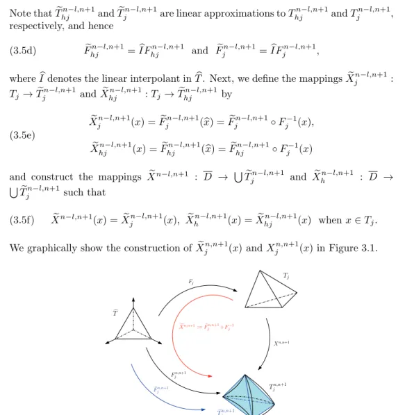
We graphically show the construction of

X

_jn,n+1

(

x

) and

X

_jn,n+1

(

x

) in Figure 3.1.

Tn,n+1

j Tj

T

Tn,n+1

j

Fj

Xn,n+1

Fn,n+1 j

Xn,n+1_:=_Fn,n+1

j ◦Fj−1

Fn,n+1 j

Fig. 3.1_. _{The points}Xn,n+1

j (x)and Xjn,n+1(x)and the mappings for the formulation of the

MLG method. X_jn,n+1(x) is in the plane face tetrahedron and X_jn,n+1(x) is in the curved face tetrahedron.

Remark

3.2. We note that if

D

is either a polygon or a polyhedron and

T

_b

is

a boundary element, i.e.,

T

b

∩

∂D

= Γ

b

⊂

∂D

, then

T

_bn−l,n+1

=

X

n−l,n+1

(

T

b

) and

T

_bn−l,n+1

=

X

n−l,n+1

(

T

b

) are also boundary elements satisfying

T

bn−l,n+1

∩

∂D

=

T

_bn−l,n+1

∩

∂D

= Γ

b

because

u

= 0 on the boundary; for the same reasons, the

inter-section of

T

_hbn−l,n+1

with

∂D

is also Γ

b

; consequently,

D

=

∪

T

jn−l,n+1

=

∪

T

n−l,n+1 hj

.

However, if

∂D

were a curved boundary, then by construction,

T

_bn−l,n+1

∩

∂D

= Γ

b

would be a curved face which, in general, is diﬀerent from the boundary face

Γ

n_b−l,n+1

of

T

_hbn−l,n+1

because the latter is a straight

d

−

1 simplex. Nevertheless,

Γ

n_b−l,n+1

in-tersects Γ

b

at its vertices. All the developments that follow are still valid for the case

with curved boundary if one makes additional assumptions and uses the techniques

of [4].

(8)

3.2.2. Calculation of

_T

j

u

n−l

h

(

X

hn−l,n+1

(

x

))

· v

h

(

x

)

dx, l

= 0

,

1. The

evaluation of the element integrals is usually done numerically by applying a

quadra-ture rule of high order, so as to maintain both the stability and the accuracy that the

method would possess if the integrals were calculated exactly. Since

u

n_h−l

∈

X

h

,

u

n_h−l

(

x

) =

M

i=1

U

_in−l

φ

i

(

x

)

,

where

{

φ

i

}

Mi₌₁

is the set of global basis functions of

X

h

and

U

in−l

=

u

n−l

h

(

x

i

), with

x

i

being the

i

th mesh node. The restriction of

u

n_h−l

on the element

T

j

is written as

u

n_h−l

(

x

)

|

T_j

=

ne

k=1

U

_kn₍−_j₎l

ϕ

(_kj)

(

x

)

,

where

ne

is the number of velocity nodes in

T

j

,

k

(

j

) denotes the global number of

the node of the mesh

D

h

that is the

k

th node of

T

j

, and

{

ϕ

( j) k

}

ne

k=1

is the set of local

basis functions for the element

T

j

. As is customary in the ﬁnite element technique, we

employ the element of reference

T

to calculate the integral over the element

T

j

. Thus,

assuming that for

x

∈

T

j

,

X

n₋l,n₊₁

h

(

x

) is in some simplex

T

i

of the ﬁxed partition

D

h

, in general

T

i

=

T

j

, then

u

_hn−l

(

X

_hn−l,n+1

(

x

)) =

ne

k=1

U

n−l k₍i₎

ϕ

(i₎

k

(

X

n−l,n+1

h

(

x

)), and

taking

v

h

(

x

) =

ϕ

( j)

p

(

x

)

,

1 ≤

p

≤

ne

, we have

Tj

u

n_h−l

(

X

_hn−l,n+1

(

x

))

· v

h

(

x

)

dx

=

ne

k=1

U

_kn₍−_i₎l

Tj

ϕ

(_ki)

(

X

_hn−l,n+1

(

x

))

ϕ

(_pj)

(

x

)

dx.

By (3.5e) and the assumption

X

_hn−l,n+1

(

x

)

∈

T

i

,

T_j

ϕ

(_ki)

(

X

_hn−l,n+1

(

x

))

ϕ

(_pj)

(

x

)

dx

=

T

ϕ

k

(

z

)

ϕ

p

(

x

)

∂F

j

∂

x

d

x,

where

z

:=

F

_i−1

◦

F

_hjn−l,n+1

(

x

). Finally, we approximate the integrals over

T

by high

order quadrature rules as

T

ϕ

k

(

z

)

ϕ

p

(

x

)

∂F

j

∂

x

d

x

meas

(

T

j

)

nqp

g=1

g

ϕ

k

(

z

g

)

ϕ

p

(

x

g

)

,

where

nqp

denotes the number of weights,

g

, and points,

x

g

, of the quadrature rule.

Remark

3.3. _{Note that in order to calculate the integrals it is necessary to deﬁne}

the triangle

T

_hjn−l,n+1

; this is done by computing at time

t

n−l

the points

X

hn−l,n+1

(

a

(j)

i

)

as solutions of (3.4); this means that the number of departure points to be calculated

every time step is

N V

, the number of vertex nodes, whereas in the conventional LG

method such a number is

N E

×

nqp

, which is much larger than

N V

because

nqp

is

quite large in high order quadrature rules, in particular in three-dimensional problems.

Since the integration of (3.4) and the identiﬁcation of the element that contains the

solution point are costly parts of the method, the MLG methods are more eﬃcient in

terms of CPU time than the conventional LG methods.

(9)

3092

4. Convergence of the MLG–BDF2 method.

In this section we perform

the error analysis of the method following a step by step approach. First, we

re-call auxiliary results concerning the convergence of the semidiscrete Stokes problem;

second, we study the error of the approximation of the departure points and some

related results, considering that the system (3.4) is integrated by a Runge–Kutta

scheme of order

r

≥

2; third, we end up establishing the convergence of the method

in the

l

∞

(

L

2

(

D

)) and

l

∞

(

H

1

(

D

)) norms for the velocity and

l

2

(

L

2

(

D

)) norm for the

pressure. In the developments that follow we need the ﬁnite dimensional space

Vh

deﬁned as

Vh

=

{

v

h

∈

Xh

: (div

v

h

, q

h

) = 0

∀

q

h

∈

M

h

}

.

Let (

u

(

t

)

, p

(

t

)) be the weak solution to (2.1). We deﬁne

w

h

: [0

, T

]

→

Xh

and

μ

h

: [0

, T

]

→

M

h

as the solution of the semidiscrete Stokes problem

(4.1)

⎧

⎨

⎩

ν

(

∇

(

u

(

t

)

−

w

h

(

t

))

,

∇

v

h

)

−

(

p

(

t

)

−

μ

h

(

t

)

,

div

v

h

) = 0

∀

v

h

∈

Vh

,

(div(

u

(

t

)

−

w

h

(

t

))

, q

h

) = 0

∀

q

h

∈

M

h

.

We have the following results (see [11, Chap 2]).

Lemma 4.1.

Let

u

∈

L

γ

(

V

∩

H

s+1

(

D

))

and

p

∈

L

γ

(

L

2₀

(

D

)

∩

H

s1+1

(

D

))

,

γ

∈

[1

,

∞

]

. Then there exist positive bounded constants

C

₇

and

C

₈

independent of

Δ

t

and

h

such that

(4.2)

u

−

w

h

_Lγ₍_L2₍D))

+

h

u

−

w

h

_Lγ₍_H1₍D))

+

p

−

μ

h

Lγ₍L2(D))

≤

C

₇

h

s+1

_u

Lγ₍_Hs+1₍D₎₎

+

C

₈

ν

h

s1+2

_p

Lγ₍Hs₁₊₁₍D₎₎

.

Besides this lemma we need the following one that can be found in [12].

Lemma 4.2.

Let the domain

D

be such that for

b > d

and

g

in

L

b

(

D

)

, the solution

(

u, p

)

of the Stokes problem

−

ν

Δ

u

+

∇

p

=

g,

div

u

= 0

in

D

,

u

|

∂D

= 0

is in

W

2,b

(

D

)

×

W

1,b

(

D

)

with continuous dependence on

g

, and assume that

D

h

is a

quasi-uniform regular partition of

D

. If

(

u, p

)

∈

L

γ

(

W

1,∞

(

D

))

×

L

γ

(

L

∞

(

D

))

, there

is a constant

C

independent of

h, u

, and

p

such that

(4.3)

∇

(

u

−

w

h

)

_L∞₍D)

+

p

−

μ

h

L∞(D)

≤

C

inf

₍v_h,q_h)∈X_h×M_h

∇

(

u

−

v

h

)

_L∞₍D)

+

p

−

q

h

L∞(D)

.

We introduce the notations

u

t

:=

∂u_∂t

and

D

tk

u

:=

Dku

Dtk

,

k

≥

1. For the Taylor–

Hood elements,

l

=

m

−

1; speciﬁcally, for the

P

₂

/P

₁

element,

m

= 2 and

l

= 1. As

for the mini-element,

l

= 1, whereas the polynomials for the velocity in an element

T

belong to

P

₁

(

T

)

spanΠ

d_i₌₁+1

ϕ

i

; however, in the velocity error estimates for this

element,

m

= 1; see [11]. To proceed with the analysis we state the following regularity

hypotheses:

(R1)

u

0

∈

H

m+1

₍

_D

₎

_∩

_W

2,∞

₍

_D

₎

_∩

_V

_.

(R2)

u

∈

L

∞

(

V

∩

H

m+1

(

D

)

∩

W

2,∞

₍

_D

₎₎

_∩

_C

₍

_C

0,1

₍

_D

_)),

_u

t

∈

L

2

(

V

∩

H

m+1

(

D

));

D

_t2

u

; and

D

3_t

u

∈

L

2

(

L

2

(

D

));

p

∈

L

∞

(

H

m

₍

_D

₎

_∩

_L

2

0

(

D

)

∩

L

∞

(

D

)); and

p

t

∈

L

2

(

H

m

(

D

)).