www.nat-hazards-earth-syst-sci.net/14/1309/2014/ doi:10.5194/nhess-14-1309-2014
© Author(s) 2014. CC Attribution 3.0 License.
Seismic hazard of the Iberian Peninsula: evaluation with kernel
functions
M. J. Crespo1,3, F. Martínez2,3, and J. Martí1,3
1Universidad Politécnica de Madrid, ETSI Minas, Calle de Ríos Rosas, 21, Madrid, Spain
2Universidad Politécnica de Madrid, ETSI Caminos, Canales y Puertos, Calle Profesor Aranguren S/N, Ciudad Universitaria, Madrid, Spain
3Principia, Velázquez, 94, 28006 Madrid, Spain
Correspondence to: M. J. Crespo ([email protected])
Received: 31 May 2013 – Published in Nat. Hazards Earth Syst. Sci. Discuss.: 2 August 2013 Revised: 3 February 2014 – Accepted: 7 April 2014 – Published: 23 May 2014
Abstract. The seismic hazard of the Iberian Peninsula is analysed using a nonparametric methodology based on statis-tical kernel functions; the activity rate is derived from the cat-alogue data, both its spatial dependence (without a seismo-genic zonation) and its magnitude dependence (without using Gutenberg–Richter’s relationship). The catalogue is that of the Instituto Geográfico Nacional, supplemented with other catalogues around the periphery; the quantification of events has been homogenised and spatially or temporally interre-lated events have been suppressed to assume a Poisson pro-cess.
The activity rate is determined by the kernel function, the bandwidth and the effective periods. The resulting rate is compared with that produced using Gutenberg–Richter statistics and a zoned approach. Three attenuation relation-ships have been employed, one for deep sources and two for shallower events, depending on whether their magnitude was above or below 5. The results are presented as seismic hazard maps for different spectral frequencies and for return periods of 475 and 2475 yr, which allows constructing uniform haz-ard spectra.
1 Introduction
The seismic design of structures requires the definition of an adequate seismic action for the site. In Spain the offi-cial information for reference in this respect is the seismic hazard map included in the Spanish seismic code NCSE-02 (Ministerio de Fomento, 2003), already about a decade
old and referring only to the Spanish territory. At about the same time, Peláez-Montilla and López-Casado (2002) presented a seismic hazard analysis (SHA) for the entire Iberian Peninsula based on the methodology by Frankel (1995). Since then, several regional studies within the Iberian Peninsula have been carried out: for the south-east of Spain (García-Mayordomo et al., 2007, and Gaspar-Escribano et al., 2008), for Andalusia (Benito et al., 2010), for the north of the Iberian Peninsula (Secanell et al., 2008, and Gaspar-Escribano et al., 2011), for Portugal (Vilanova and Fonseca, 2007, and Sousa and Campos, 2009), and finally Mezcua et al. (2011) have presented PGA (peak ground ac-celeration) results for the Spanish territory within the Iberian Peninsula.
Although national norms may lose jurisdiction at political boundaries, technical findings are not sensitive to them. It is therefore decided that the present study should cover the entire Iberian Peninsula.
In recent times important advances have taken place in several areas that strongly influence an SHA.
– New evaluation methods have been proposed, some of which forego the use of seismogenic zones (Frankel, 1995; Woo, 1996a).
– Research on attenuation models has led to better models and to guidance on their use.
At the same time, the goals pursued by seismic design have also evolved in a number of aspects.
– A design seismic input may now be required at unpopu-lated locations, such as maritime areas or coastal zones. – The characterisation of the seismic input is expected to be more sophisticated; PGA and the felt intensity are no longer sufficient, and uniform hazard spectra (UHSs) are required.
– Increasingly, the design of structures and facilities is based on more than one level of probability, each level associated with a given set of performance require-ments.
As a consequence, it is appropriate to reevaluate the seismic hazard for the whole Iberian Peninsula, incorporating all re-cent advances and satisfying the new engineering needs.
The present work was developed in the context of the PhD thesis by Crespo (2011). Since then, the Spanish Instituto Ge-ográfico Nacional has carried out a re-evaluation of the na-tional seismic hazard map incorporating the present method-ology (Ministerio de Fomento, 2013).
2 Methodology
The methodology employed is inspired by the non-parametric density estimation (NPDE). In NPDE, the objec-tive is to find the density function from which a given sample derives, without specifying a priori a specific shape for the density function, such as a normal distribution or a gamma one; instead, the shape of the distribution is expected to be provided by the sample itself.
The method consists in centring a density function on each element of the sample, adding all such functions and normal-ising their sum. It was initially proposed by Fix and Hodges (1951), but a more recent and very clear description is pro-vided by Silverman (1986).
The specific application of NPDE to seismic data was pro-posed by Vere-Jones (1992). Later on, Woo (1996a, b) pre-sented a way of using kernel functions for modelling seismic activity rates in SHA.
The mathematical definition of density estimated with ker-nel functions is as follows:
fn(x)= 1
nH2 n
X
i=1
K
x−x
i
H
, (1)
wherenis the number of elements in the sample,H is the bandwidth, which is a measure of the separation between sample elements,Kis the kernel function, andxi is the po-sition of eventi.
For generating a seismic activity rate density λk, two changes are introduced in the previous expression:
– The normalisation with respect to the number of events
n is omitted; thus the result is expressed in terms of number of events.
– Each kernel function is divided by an effective period of detectionT, so the density of events is per unit time. With the above two changes, the expression becomes
λk(M,x)= 1 [H (M)]2
n
X
i=1
K x−xi
H
T (xi)
. (2)
The effective periodT is a measure of the detection probabil-ity of that event in past times. As noted in Eq. (2), each event can be assigned a different effective periodT, which makes the methodology very versatile. Typical event characteristics on which the effective period usually depends are the event magnitude, the time of occurrence and the characteristics of the epicentral location (onshore, offshore, unpopulated area at the time of occurrence, etc.), but other factors affecting the probability of the event being detected can also be incorpo-rated through the effective period.
The resulting activity rate densityλkdepends on location as well as magnitude through the bandwidthH. As can be seen, it is a summation of kernel functionsKplaced on each event of the catalogue with coordinatesxi. Each function is weighted with an effective detection periodT; the normali-sation is achieved through the bandwidthH, which depends on the distance between events, as it will be seen later in Sect. 5.1. The kernel function, the effective detection periods and the bandwidth are the three main parameters influencing the activity rate density.
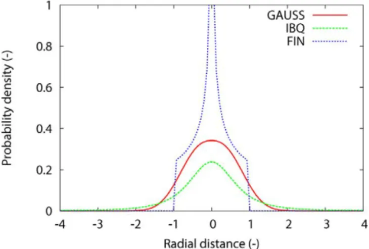
Several kernel functions have been proposed for the cases where the sample is of seismic type, specifically the Gaus-sian kernel, the inverse bi-quadratic (IBQ) and a finite one that has zero values for distances greater than one bandwidth. The first two kernels were proposed by Vere-Jones (1992); later on, Woo (1996a) proposed employing the IBQ and al-ternatively a finite one. All three types of kernels can be seen in Fig. 1. The kernels are axially symmetric.
The IBQ kernel originally proposed by Woo (1996b), apart from being the one in common to the proposals by Vere-Jones (1992) and Woo (1996a), has been employed here. Its mathematical expression is
KIBQ(x)=
λ
IBQ−1
π
1+xTx−λIBQ, (3)
whereλIBQ is a parameter greater than 1 for which Vere-Jones (1992) suggests values between 1.5 and 2.0.
Figure 1. Probability densities of various kernel functions: the
Gaussian kernel (GAUSS), the inverse bi-quadratic kernel (IBQ), and a finite kernel that vanishes in one bandwidth (FIN).
capture correctly the temporal activity rate without eliminat-ing any event, since this would affect the spatial distribution of the activity rate density. Details on the derivation of the effective periods in this case are presented in Sect. 5.2.
The bandwidth is assumed to depend on magnitude through an exponential law. The relation proposed by Woo (1996a) was
H (M)=cexp(dM), (4)
wherecandd are parameters to be adjusted, andM is the magnitude, or the measure employed for the quantification of the event’s size.
This type of dependency follows the standard form of log-arithmic correlation between the magnitude and other seis-mic parameters such as, for instance, the fault length. Again, specific details on the derivation of the parameterscanddin Eq. (4) are presented in Sect. 5.2.
With the activity rate density already estimated and the attenuation model, the rate of occurrence of different levels of ground motionyj can be derived as follows:
λyj = Z
Mmax
Z
Mmin
PY > yj|M,x
λk(M,x)dMdx. (5)
The rate of occurrence is computed with Eq. (5), and it fol-lows exactly the summation specified in Eq. (2) for the con-struction of the seismic activity rate density; the procedure is quite simple though very intensive in calculations since for each magnitude it goes through the entire catalogue. The kernel function is given in Eq. (3) and the shape of the band-width in Eq. (4). These four equations give all the mathemat-ical input needed to understand the construction of the rate of occurrence.
The seismic activity rate density has to be calculated for the entire area that is susceptible to generating earthquakes
that are relevant for the location studied. The extension of this area depends on the minimum threshold of ground mo-tion of interest and the maximum magnitude in the area; with these data and the attenuation relation, it is possible to esti-mate the extension of the area where the seismic activity rate density is needed.
Once the rate of occurrence of different levels of ground motion has been obtained, the seismic hazard curve at the site is derived assuming a Poisson process.
This methodology was originally implemented by Woo (1996b) in the Fortran program KERFRACT. In the context of the work by Crespo (2011), the code was modified in sev-eral aspects that are explained in detail in her work. However, the most important changes affecting the calculation algo-rithm are as follows:
– For each magnitude being integrated, the decision of whether an event is considered or discarded when com-puting the seismic activity is made dependent on the uncertainty associated with the event magnitude. This change is especially relevant for historical events that have large magnitude uncertainties.
– The computation of the activity rate may have the depth as an additional variable of integration.
This methodology has been already applied in the past in many parts of the world. Apart from the authors (Crespo and Martí, 2002; Crespo et al., 2003, 2007), Secanell et al. (2008) also employed it for studying the Pyrenean region, Menon et al. (2010) for South India, and Goda et al. (2013) for the UK.
A question may be posed as to the reliability of this de-scription of the activity rate and its relative merits in compar-ison with traditional zoned procedures (Stein et al., 2011). Several considerations may be offered in this respect. A first advantage over zoned procedures comes from avoiding the imposition of constant seismic activity over zones with step-wise jumps across boundaries; this is particularly signifi-cant in areas of low to medium activity, with no clear as-sociation between seismicity and geological features, where the delineation of zones is a primarily subjective matter, which has a strong influence on the results. In this respect Giner et al. (2002) presented five different zonifications, con-structed by different authors for the same area of Spain, that produce very different hazard results.
Further, as shown by the results presented here, there are areas like south-eastern Spain and the Pyrenean region where the zoneless approaches arrive at significantly higher accel-eration values than the traditional methodologies. The re-cent activity felt in south-eastern Spain has been consider-ably higher than expected from available hazard maps, which again seems to confirm the limitations of the zoned approach. A similar situation has arisen in Italy regarding the recent ac-tivity around L’Aquila and Emilia-Romagna (G. Woo, per-sonal communication, 2013).
3 Seismic catalogue 3.1 Sources
The main catalogue used in the study is the seismic database maintained by the Spanish Instituto Geográfico Nacional (IGN, 2010): more than 95 % of the final catalogue employed here is constituted by events from the IGN database. How-ever, some areas that are relevant for the seismic hazard of the Iberian Peninsula are not fully covered by the IGN catalogue. This is especially true for the south-east of France; also some large events in north-western Italy may influence the seis-mic hazard of the north-east of Spain. The IGN catalogue has been completed with data from two international organ-isations (USGS, 2011; ISC, 2010), data from the catalogues of neighbouring countries (BRGM, 2010; Gruppo di lavoro CPTI, 2004) and published works that describe the seismicity of surrounding regions (Vilanova and Fonseca, 2007; Peláez et al., 2007).
Nearly 60 000 earthquakes have been considered, which include all magnitudes/intensities registered and dependent events. Most of them, more than 97 %, come from the IGN catalogue; some 1500 were added from the ISC, most of them located in France and in the north of Africa and belong-ing to the instrumental period; finally, just 45 earthquakes were taken from the USGS, all of them catalogued as “sig-nificant events” and located outside the Spanish territory in areas not covered by the IGN catalogue.
The most ancient event with an assigned intensity dates back to 1048 and belongs to the IGN catalogue, while the most recent events considered date from November 2010. 3.2 Magnitude unification
The quantification of events has to be homogeneous through-out the catalogue. The homogenisation has been conducted in terms of magnitude, specifically the moment magnitudeMw, which is becoming the standard measure for seismic events and is the one used in the majority of modern attenuation re-lations. Some 10 % of the events in the IGN catalogue are only quantified with epicentral intensity, as is frequently the case for events from the historical period. For these histor-ical earthquakes, if they had an assigned magnitude either by the IGN (2010) or by specific studies (Martínez-Solares
and López-Arroyo, 2004; Vilanova and Fonseca, 2007), that value has been considered; in the other cases the correlation by L. Cabañas (personal communication, 2010) specifically developed for the Iberian Peninsula has been employed:
Mw=1.525+0.578I0 σ=0.404, (6)
whereMwis the moment magnitude,I0is the epicentral in-tensity, andσ is the standard deviation.
During the instrumental period most events have an as-signed magnitude; generally this magnitude is eithermb or
mbLg, and since 2002, some of them have also had a mo-ment magnitude. The type of magnitude is specified in the catalogue provided by the IGN (2010). The conversion of both epicentral intensity and magnitude mb or mbLg into moment magnitude has been carried out using correlations specifically developed for the Iberian Peninsula by the IGN (L. Cabañas, personal communication, 2010). Specifically, three subsets of earthquakes are considered, each one hav-ing a different correlation.
– For earthquakes characterised with magnitudemb,
Mw= −1.576+1.222mb σ=0.355. (7)
– For earthquakes before March 2002 and characterised with magnitudembLg,
Mw=0.258+0,980mbLg σ=0.251. (8)
– For earthquakes after March 2002 and characterised with magnitudembLg,
Mw=0.644+0.844mbLg σ=0.235. (9)
Moment magnitudes already assigned by the IGN (2010) have been maintained, and some other moment magnitudes from the literature have also been incorporated (Stich et al., 2003, 2010).
As will be explained in Sect. 6, the magnitude integration range starts atMw=3.5. Magnitude uncertainties are con-sidered on an event-by-event basis assuming a Gaussian dis-tribution with the mean being the magnitude in the catalogue. Hence it is necessary to consider lower-magnitude events in the process of integration. In this case the minimum magni-tude threshold in the catalogue isMw=3.0.
3.3 Dependent events
– The window size depends on the event magnitude ac-cording to the indications given by Peláez et al. (2007); namely, forMw=3.0 the spatio-temporal window was of 20 km and 10 days, and 100 km and 900 days for
Mw=8.0.
– The catalogue is scanned in decreasing magnitude or-der, so that in the potential series the first event identi-fied is always the main shock (Crespo, 2011).
As a result of the pruning process conducted, 36 % of the events were considered dependent events (either foreshocks or aftershocks) and were discarded from the catalogue. 3.4 Uncertainties
The methodology used requires the catalogue to incorporate uncertainties with respect to magnitude as well as to location (epicentre and depth).
Regarding magnitude, the uncertainties quoted in the var-ious catalogues have been taken into account. When using a correlation, its uncertainties have been combined with those in the catalogue. It should be pointed out that the correlations provided by the IGN (L. Cabañas, personal communication, 2010) have been derived with an RMA (reduced major axis) methodology which takes into account the variability of the two variables being adjusted. These correlations have been published by the IGN (Ministerio de Fomento, 2013).
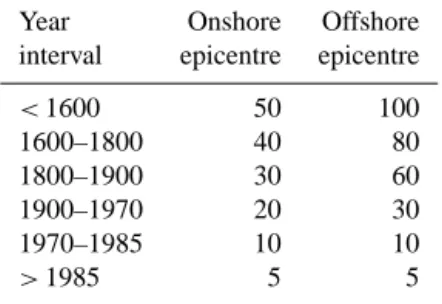
As for the location uncertainty, the catalogues provide this type of information for many earthquakes, especially in the instrumental period. For events lacking this information in the catalogue, an uncertainty has been estimated. It seems logical that this uncertainty be higher for events that oc-curred at older times, and that it be higher for epicentres at sea. The uncertainties assigned to the epicentral location follow the recommendations by G. Woo (personal commu-nication, 2000) and are also in agreement with the sugges-tions by other authors (Giner, 1996; Molina, 1998; García-Mayordomo, 2005). The uncertainties finally assigned to sea and land epicentres appear in Table 1.
4 Attenuation model
Major research on the attenuation of ground motion has been taking place for at least half a century, but important ad-vances have been produced recently, both in relation to the number of models available and to their functional forms.
Very relevant work has also been conducted on the criteria for selecting attenuation models when conducting an SHA. Cotton et al. (2006) proposed a series of seven criteria that in practice were rather difficult to satisfy. Later on, Bommer et al. (2010) reformulated the criteria into a set of 10 recom-mendations.
Attenuation studies at present tend to focus on medium to high magnitudes, a range that is representative of only a small
Table 1. Uncertainties (km) in epicentre location.
Year Onshore Offshore
interval epicentre epicentre
<1600 50 100
1600–1800 40 80
1800–1900 30 60
1900–1970 20 30
1970–1985 10 10
>1985 5 5
fraction of the seismicity in low to medium seismicity areas such as the Iberian Peninsula. Bommer et al. (2007) alerted to the problems that can arise when an attenuation model is em-ployed out of the range for which it was developed. They also presented some preliminary results obtained with an attenu-ation model that employs a database spanning magnitudes 3.0–7.5; their results in the lower range are consistent with those of Bragato and Slejko (2005).
In the present work, three different attenuation models have been employed:
– Ambraseys et al. (2005) for shallow earthquakes with moment magnitudes above 5.0
– Bragato and Slejko (2005) for shallow earthquakes with moment magnitudes below or equal to 5.0
– Youngs et al. (1997) for deep earthquakes.
The boundary between shallow and deep earthquakes has been fixed at 35 km, all deep earthquakes occurring between 35 and 200 km, except for a few around Granada which are around a 600 km depth. These very deep earthquakes are not included in the calculation. In the same way, deep earthquakes are accounted for just for magnitudes above
Mw=5.0, which is the range of applicability of the atten-uation relation and a sensible lower bound for deep earth-quakes; hence, deep earthquakes around the Pyrenean region and many around the south of the peninsula also fall outside the group of interest.
becomes smaller. In an area of medium–low seismicity like the Iberian Peninsula, the maximum spectral amplification in terms of acceleration is expected to appear at low periods. Since one of the objectives of the work was to capture this spectral amplification, the sampling provided by Ambraseys et al. (2005), smaller than other attenuation models and con-sistent with that of Bragato and Slejko (2005), was consid-ered more appropriate. Additionally it is consistent with the model by Bragato and Slejko (2005), with which it will be combined. In relation to the magnitude, it is not important that the model by Ambraseys et al. (2005) does not include the non-linear magnitude dependence proposed by Bommer et al. (2010), because it will only be used in part of the mag-nitude range.
The number of attenuation models generated with databases that cover the low magnitude range, specifically below 5.0, is considerably smaller. That by Bragato and Sle-jko (2005) is one of them and, as already mentioned, is con-sistent with the preliminary results presented by Bommer et al. (2007). Additionally, it satisfies 8 out of the 10 cri-teria proposed by Bommer et al. (2010), the remaining two being of lesser importance since the model will be employed in only part of the magnitude range. The minimum magni-tude at which the integration of the seismic activity rate den-sity begins isMw=3.5. This value was finally adopted af-ter repeated calculations showed that further lowering of this threshold only affects the results in areas with lower hazard and for return periods below 475 yr.
There are studies based on macroseismic intensity data that conclude different attenuations for different regions within the peninsula (Sousa and Oliveira, 1996; López Casado et al., 2000). Here, only one attenuation model for shallow seismicity is employed for the whole Iberian re-gion; this decision follows the recommendations by Bom-mer et al. (2010), who claim that there is no strong evi-dence for persistent regional differences in ground motions among tectonically comparable areas. Their recommenda-tions are based on the works by Douglas (2007) and Stafford et al. (2008), which rely on recorded strong ground motions rather than macroseismic data.
Attenuation models for deep earthquakes are very scarce, and those available refer to subduction zones like Chile, west coast of Mexico, Peru or Japan. To account for deep seis-micity in the calculations, a model must be used that in-cludes focal depth as an independent variable; there is then little choice other than a subduction model, even if the tec-tonic patterns represented are not the ideal ones. Among the available subduction models, that by Youngs et al. (1997) was selected because it scores higher on the list by Bommer et al. (2010).
The attenuation models have to be harmonised for consis-tency in their input parameters and in the results produced. In relation to magnitude, the catalogue had been homogenised in terms ofMw, which is already the measure employed by Ambraseys et al. (2005) and Youngs et al. (1997). The model
by Bragato and Slejko (2005) was originally developed in local Richter magnitudeMLbut, for the range in which this model is applied here, both magnitudes can be considered equivalent, as also assumed by Bommer et al. (2007).
The distance considered is the epicentral distance. The model by Bragato and Slejko (2005) is based on that dis-tance. That by Ambraseys et al. (2005) employs the Joyner– Boore (JB) distance but, for moderate seismicity, the JB distance can be assumed to be equal to the epicentral one. Youngs et al. (1997) make use of a similar equivalence between the epicentral distance, adequately combined with depth, and the distance to the rupture surface originally em-ployed in the model.
The type of soil for which the results are derived is “stiff soil” with a shear wave velocity between 360 and 750 m s−1: this is the range for which the Bragato and Slejko (2005) model was investigated in detail and is also one of the soil types considered by Ambraseys et al. (2005). It corresponds also to one of the two types of ground studied by Youngs et al. (1997).
Finally, the acceleration measure used in the regression, which is also the output acceleration, may vary; indeed all three models use different measures of acceleration. The present results employ the same measure as Ambraseys et al. (2005), which uses the maximum horizontal compo-nent. For Bragato and Slejko (2005) a conversion has been carried out using their own model guidelines, and in the case of Youngs et al. (1997), the correlations by Beyer and Bom-mer (2006) have been incorporated.
Figures 2 and 3 present part of the attenuation model con-structed for shallow seismicity, which includes the correla-tions by Ambraseys et al. (2005) and Bragato and Slejko (2005), with the aforementioned modifications. As can be seen, the combination of these two models, with the appro-priate homogenisation, yields good continuity at theMw= 5.0 boundary. As a qualitative verification, the maximum spectral acceleration (SA) can be seen to move towards the lower frequencies with increasing magnitude, as could be ex-pected.
5 Seismic activity rate
The seismic activity rate is calculated according to Eq. (2). The kernel function employed is the IBQ, as stated in Sect. 2. In this section particular choices made for the determina-tion of the bandwidth and the effective detecdetermina-tion periods are described first, which are the two fundamental elements on which the seismic activity rate relies.
Figure 2. Attenuation of PGA for shallow earthquakes and stiff soil
sites. Magnitudes above 5 have been attenuated with Ambraseys et al. (2005) and magnitudes equal or below 5 with Bragato and Slejko (2005).
original implementation by Woo (1996b) did not offer the possibility of retrieving them. However, it has been consid-ered a useful exercise in order to help understand the differ-ences between the traditional and the kernel approach. 5.1 Bandwidth
The bandwidthH (Mw)depends on magnitude as indicated in Eq. (4). This type of logarithmic relation between moment magnitude and bandwidth is commonly assumed to be appli-cable between moment magnitude and other seismic param-eters.
The derivation ofcandd is performed via a least-square fit:
– Events are classified in groups according to their mag-nitude.
– For each event, the distance to the nearest epicentre within the same magnitude range is determined. – All minimum distances calculated for each magnitude
range are averaged.
– A least-square fit is conducted in order to obtain the two parameters,candd, that appear in Eq. (4).
This methodology has been previously applied at several sites (Crespo and Martí, 2002; Crespo et al., 2003, 2007).
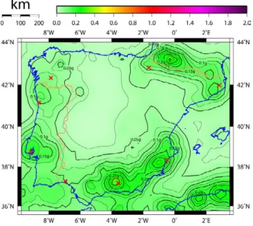
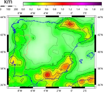
The derivation of the parameterscandd is done indepen-dently for shallow and deep earthquakes. If Eq. (4) is ad-justed using the complete catalogue, the resulting correlation is that presented in Fig. 4. However, since the fit is conducted at all points where the hazard is computed, the spatial distri-bution of c can also be produced, as shown in Fig. 5. As reflected in the figure, c shows stable values between 0.25 and 0.50 for the areas of higher activity. In the central part of
Figure 3. Attenuation of shallow earthquakes for stiff soil sites and
10 km of epicentral distance. Magnitudes above 5 have been atten-uated with Ambraseys et al. (2005) and magnitudes equal or below 5 with Bragato and Slejko (2005).
the peninsula and in the Balearic Islands, the values increase to around 3.0, which is consistent with the fact that a lower seismicity implies earthquakes more distant from each other. 5.2 Effective detection periods
The effective detection periods, parameterT (xi) in Eq. (2), have been calculated considering whether an earthquake is shallow or deep, and for the shallow ones, whether the epi-centre is on land or at sea.
The magnitude and year of occurrence of each earthquake are taken into account for determining the effective period of the earthquake as follows:
– History is divided into time intervals as a function of the means of detection available at each time.
– For each interval with duration Di and each level of magnitude, a probability of detectionpimis estimated. – A reference yearAmis established for each magnitude
level:
Am=A0−
X
i
pimDi, (10)
whereA0is the most recent year with records.
Figure 4. Derivation of the bandwidth parameters using the
cata-logue data, separately grouped into shallow and deep events.
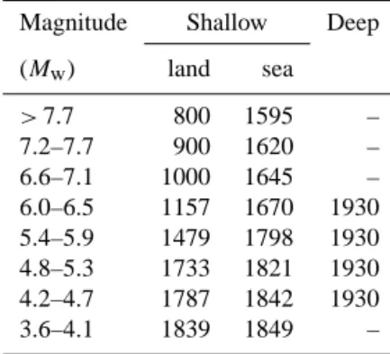
Table 2 shows the reference years obtained by the previous procedure for the calculation of the detection periods. 5.3 Computation of the seismic activity rate
Having defined the kernel function K(x), the bandwidth
H (Mw), and the effective detection periodsT (xi), the activ-ity rate can be calculated using Eq. (2). The resulting activactiv-ity depends on location and magnitude.
For a given magnitude level, the seismic activity rate can be contoured; similarly, for a given location, the activity rate can be plotted. This second result is equivalent, except for a factor of area, to the traditional activity rate derived with the Gutenberg and Richter (1944) relationship. Figure 6 shows, for the south-west of the Iberian Peninsula, a contour map of the activity rate for earthquakes with magnitude above 3.5, which is consistent with the seismicity of this area. This plot constitutes the first type of intermediate results that can be produced. Although these types of results have been obtained for the whole Peninsula, we include here the ones for the south-west, which is one of the most illustrative areas.
Figure 7 shows plots of the activity rate for the four lo-cations marked in the previous map. These curves repre-sent the number of earthquakes per unit area and per year for a given location, similar to the concept used in the Gutenberg–Richter relationship. However, here this is just a by-product of the calculations, while in the traditional proce-dure it is a necessary step on which some assumptions, like the analytical shape of the correlation, will be based. In the present case, the shape, not necessarily linear, arises directly from the catalogue data.
The graphs in Fig. 7 include also a linear fit of the activity rate derived from the calculations. The slope of this line, re-ferred to here asbk, may be compared with thebparameter
Figure 5. Distribution of the bandwidth parameterc; the higher val-ues (red and purple) that appear in low seismicity areas (central Iberian Peninsula and Balearic Islands) indicate a greater distance between events of similar size.
Figure 6. Annual rate of occurrence of events per km2withMw>
3.5. Points A to D indicate the locations where the activity is plotted in Fig. 7.
of the Gutenberg–Richter relationship. For each point of the map, similar fits could be performed leading to a value of the
bkparameter; the results are plotted in Fig. 8. As can be seen, the values found forbk are consistent with the typical ones already predicted by Gutenberg and Richter (1944) for theb
M. J. Crespo et al.: Seismic hazard at the Iberian Peninsula 1317
Table 2. Reference years for different magnitudes and types of
events.
Magnitude Shallow Deep
(Mw) land sea
>7.7 800 1595 –
7.2–7.7 900 1620 –
6.6–7.1 1000 1645 –
6.0–6.5 1157 1670 1930
5.4–5.9 1479 1798 1930
4.8–5.3 1733 1821 1930
4.2–4.7 1787 1842 1930
3.6–4.1 1839 1849 –
6 Results and discussion 6.1 General considerations
Once the activity rateλk has been calculated (Sect. 5) and an attenuation model has been adopted (Sect. 4), the seismic hazard can be calculated.
The magnitude integration range for shallow seismicity starts at Mw=3.5 and for deep earthquakes atMw=5.0. The lower limit for integration depends on the return period of interest and on the minimum acceleration levels that need to be correctly captured. In the present case it was verified that, for the 475 yr return period, the integration should start atMw=3.5 if accelerations as low as 0.04gmust be deter-mined: using a lower limit for integration does not change the results significantly, while higher values would affect the results. This observation confirms the stability and consis-tency of the attenuation model constructed. The question of whether or not the minimum accelerations derived are of en-gineering interest should be decided by the engineer who will be making use of them and will depend on the type and pur-pose of the calculation being performed. What has to be guar-anteed at this stage is that the minimum accelerations being derived are reliable, which requires an adequate selection of the magnitude integration threshold.
The upper limit of integration arises from the maximum magnitude recorded in the catalogue and its uncertainty, specifically,Mwi+2σMwi,σMwi being the uncertainty
asso-ciated with event i. Again, it was verified that the results are not sensitive to increases in this upper limit, since each event contribution is weighted with the probability that its magnitude falls within the integration range, assuming a log-normal magnitude distribution.
For deep earthquakes, the range of integration used is 35 to 200 km.
1e−12 1e−11 1e−10 1e−09 1e−08 1e−07 1e−06 1e−05 0.0001 0.001
0 2 4 6 8 10
activity rate (events/km
2/year)
magnitude (Mw)
(a) Point A
1e−12 1e−11 1e−10 1e−09 1e−08 1e−07 1e−06 1e−05 0.0001 0.001
0 2 4 6 8 10
activity rate (events/km
2/year)
magnitude (Mw)
(b) Point B
1e−12 1e−11 1e−10 1e−09 1e−08 1e−07 1e−06 1e−05 0.0001 0.001
0 2 4 6 8 10
activity rate (events/km
2/year)
magnitude (Mw)
(c) Point C
1e−12 1e−11 1e−10 1e−09 1e−08 1e−07 1e−06 1e−05 0.0001 0.001
0 2 4 6 8 10
activity rate (events/km
2/year)
magnitude (Mw)
(d) Point D
Fig. 7.Activity for each of the four locations identified in Figure 6:(a)point A;(b)point B;(c)point C;(d)point D. The relation is approximately straight.Figure 7. Activity for each of the four locations identified in Fig. 6:
(a) point A, (b) point B, (c) point C, and (d) point D. The relation
is approximately straight.
Figure 8. Contours ofbk in the south-west of the peninsula. This
parameter, which arises from the calculations, is comparable to the
bparameter of the Gutenberg–Richter relationship.
6.2 Contour maps
The PGA has been calculated for a rectangular area that spans the Iberian Peninsula for return periods of 475 and 2475 yr. The resulting contours appear in Figs. 9 and 10.
Figure 9. Distribution of the accelerations obtained forT =0 s and 475 yr return period.
It is also around this return period that the contribution to the seismic activity rate arising from geological consid-erations may start being significant. Given the convergence rate between the Iberian and African plates, it is expected that faults in the Iberian Peninsula are also slow, so mor-phogenic earthquakes (hence with magnitude above 6.0–6.5) have recurrence periods of the order of few thousand years, which exceeds the period covered by the seismic catalogue: note that the first event in the catalogue dates from the fourth century BC, and the first quantified event from the fifth cen-tury AD. The explicit inclusion of geological data would be carried out adding earthquakes that are representative of the characteristic magnitude of the fault and with an effective period consistent with the fault recurrence period. This inclu-sion affects two aspects: the location where the activity rate is modelled, which concentrates around specific geometrical features or faults; and the activity rate itself, which is en-riched with geological information that the seismic catalogue does not reflect.
The effect on the distribution of the activity rate is partly incorporated using the kernel methodology: the activity rate is not uniformly spread over zones, but this is only guided by the epicentral locations. All this should be taken into account when considering the results.
Looking at the 475 yr map, the areas with higher hazard levels are Granada (south of Spain) and the French slope of the Pyrenees, where the PGA values reach 0.30g, followed by the south-east of the peninsula, around the city of Ali-cante, with a value of 0.27g. Outside the Iberian Peninsula, the area around Algiers has 0.25g. Finally, Lisbon and the north of Catalonia attain values of 0.20gand 0.15g, respec-tively.
Figure 10. Distribution of the accelerations obtained forT=0 s and 2475 yr return period.
The results for a 2475 yr return period are presented in Fig. 10. It can be seen that the distribution of the hazard is similar to that observed for 475 yr, with approximately dou-ble the acceleration values. This ratio is consistent with the dependence on the return period proposed in the Spanish seismic code (Ministerio de Fomento, 2003).
Two additional hazard maps are shown in Figs. 11 and 12: they correspond to the same return periods mentioned earlier but refer to a spectral period ofT =0.1 s. As clarified in the next section, this spectral ordinate is the more representative one for deriving the maximum spectral accelerations, which are those of the plateau. This spectral ordinate peaks in the same places as the PGA: around Granada it reaches 0.90g
for 475 yr and 1.90gfor 2475 yr.
The ratio of the plateau acceleration to the PGA for 475 yr turns out to be between 2.5 and 2.8 in most of the Iberian Peninsula (Fig. 13), which is in agreement with the value of 2.5 frequently found in seismic codes.
6.3 Uniform hazard spectra
Results were also produced in terms of uniform hazard spec-tra for the eight locations marked with red crosses in Fig. 9. They are shown in Fig. 14 for selected sites from the south of the Iberian Peninsula and in Fig. 15 for those in the north. The maximum amplification appears between periodsT =
0.1 s andT =0.15 s, which is consistent with spectra corre-sponding to low magnitudes derived directly from the atten-uation model (Fig. 3).
Figure 11. Distribution of the accelerations obtained forT =0.1 s and 475 yr return period.
Figure 12. Distribution of the accelerations obtained forT =0.1 s and 2475 yr return period.
periods for anchoring those branches were found to beT =
0.1, 0.4 and 2.0 s, respectively. However, the latter corre-sponds, in fact, to the highest period for which results are available; hence the possibility exists that a longer period might have been preferable.
6.4 Comparison with previous studies and seismic codes It is interesting to compare the results shown above with those of other recent regional studies. Benito et al. (2010) presented a study for Andalusia. The geometry of their
con-Figure 13. Maximum amplification of the accelerations for 475 yr
return period, measured by the ratio of the plateau to the PGA.
tour lines is consistent with that shown in Fig. 9, and their nu-merical values are also consistent, possibly slightly lower, af-ter correcting for the fact that their results correspond to rock conditions. For Granada the present study calculates 0.30g
(for stiff soil) while they find 0.22gfor rock; this difference may be partly explained from the consideration of different soil types.
Secanell et al. (2008) studied the area around the Pyre-nees. They used the kernel methodology proposed by Woo (1996a) in one of the branches of a logic tree. As in the pre-vious case, after correcting for the soil type, there is good consistency with the results presented here, both qualitative and quantitative.
For the area around Alicante, we calculate 0.28g, a value that is significantly higher than the one reported using zoned methods (Mayordomo, 2005; García-Mayordomo et al., 2007; Benito et al., 2006) but that is in agreement with Peláez-Montilla and López-Casado (2002), who employed a variant of the zoneless approach by Frankel (1995) working in terms of felt intensity.
For these two latter areas (Pyrenees and Alicante), good consistency is found with previous studies based on zoneless approaches but not otherwise. This suggests that the spatial gradient of the activity rate in these areas is high, so the zona-tion needed in order to represent this seismic activity rate would require small zone dimensions, which might be dif-ficult to characterise, in terms of magnitude–frequency rela-tionships, with the seismic information available.
For the area of Portugal the present study reaches 0.20g
1320 M. J. Crespo et al.: Seismic hazard at the Iberian Peninsula 0 0.5 1 1.5 2
0 0.5 1 1.5 2
SA (g)
T (s) 475 yr fit 475 yr 2475 yr fit 2475 yr
(a) Huelva 0 0.5 1 1.5 2
0 0.5 1 1.5 2
SA (g)
T (s) 475 yr fit 475 yr 2475 yr fit 2475 yr
(b) Granada 0 0.5 1 1.5 2
0 0.5 1 1.5 2
SA (g)
T (s) 475 yr fit 475 yr 2475 yr fit 2475 yr
(c) Alicante 0 0.5 1 1.5 2
0 0.5 1 1.5 2
SA (g)
T (s) 475 yr fit 475 yr 2475 yr fit 2475 yr
(d) Lisbon
Fig. 14.Comparison of uniform hazard spectra and fitted code spectra for cities in the south of the Iberian Peninsula:(a)Huelva;(b)Granada;
(c)Alicante;(d)Figure 14. Comparison of uniform hazard spectra and fitted codeLisbon. spectra for cities in the south of the Iberian Peninsula: (a) Huelva,
(b) Granada, (c) Alicante, and (d) Lisbon.
after accounting for the different soil type, the value around Lisbon would be slightly lower in our study, with a somewhat larger difference for the south of Portugal. The attenuation relationships employed by Vilanova et al. (2007) are proba-bly responsible for this discrepancy. Vilanova et al. (2007) used three different attenuation models in the branches of their logic tree, and the lowest values were derived using Ambraseys et al. (1996), not very different from Ambraseys et al. (2005) employed here. Considerably larger are the val-ues found by Peláez-Montilla and López-Casado (2002), but this is likely a consequence of the fact that they work in terms of intensity and translate the final results into accelerations.
Table 3 compares the calculated PGA values for eight cities in the Iberian Peninsula and compares them with those reported elsewhere. The locations are indicated with red crosses in Fig. 9.
Regarding the return period of 2475 yr, although it is be-coming a more frequent reference (OPCM, 2008; NRC-IRC, 2010; ASCE, 2010), no results have been published recently for it so comparisons cannot be offered.
Regarding the UHS results, the range of spectral periods with maximum amplification appears to be narrower than in-dicated by the Spanish seismic code (Ministerio de Fomento, 2003) for soil type II, which is equivalent to the stiff soil considered here; however it is in agreement with the peri-ods used to limit the plateau in Eurocode 8 (CEN, 2004) for earthquakes with magnitude belowMs=5.5.
0 0.5 1 1.5 2
0 0.5 1 1.5 2
SA (g)
T (s) 475 yr fit 475 yr 2475 yr fit 2475 yr
(a) Ourense 0 0.5 1 1.5 2
0 0.5 1 1.5 2
SA (g)
T (s) 475 yr fit 475 yr
2475 yr fit 2475 yr
(b) Pamplona 0 0.5 1 1.5 2
0 0.5 1 1.5 2
SA (g)
T (s) 475 yr fit 475 yr 2475 yr fit 2475 yr
(c) Gerona 0 0.5 1 1.5 2
0 0.5 1 1.5 2
SA (g)
T (s) 475 yr fit 475 yr 2475 yr fit 2475 yr
(d) Porto
Fig. 15.Comparison of uniform hazard spectra and fitted code spectra for cities in the north of the Iberian Peninsula:(a)Orense;(b)
Pamplona;(c)Figure 15. Comparison of uniform hazard spectra and fitted codeGerona;(d)Oporto.
spectra for cities in the north of the Iberian Peninsula: (a) Ourense,
(b) Pamplona, (c) Gerona, and (d) Porto.
Table 3. Results of PGA (g) for selected locations. Results of the present study are compared with values given by the official Spanish seismic code as well as other published studies.
PGA Other
City stiff soil NCSE-02c PM&LCd studies
(this study) (stiff soil) (for rock)
Huelva 0.10 0.10 0.16 0.19
f
0.05–0.08a
Granada 0.30 0.23 0.16–0.24 0.16–0.22a
Alicante 0.21 0.14 0.08–0.16 0.11–0.12b
Lisbon 0.21 – 0.24–0.32 0.19f
Ourense 0.09 0.04 0.04–0.08 0.10f
Pamplona 0.11 0.04 0.04–0.08 0.08–0.10e
Gerona 0.14 0.08 0.04–0.08 0.08–0.10e
Porto 0.10 – 0.04–0.08 0.10f
aBenito et al. (2010).
bGarcía-Mayordomo et al. (2007). cMinisterio de Fomento (2003).
dPeláez-Montilla and López-Casado (2002). eSecanell et al. (2008).
fVilanova et al. (2007).
that the period T =0.2 s should more likely belong to the constant acceleration branch.
Using several spectral ordinates to construct design spec-tra is probably the best way of taking advantage of all the information produced with the new attenuation models. The Italian seismic code (OPCM, 2008) is a good example in Eu-rope.
7 Summary and conclusions
A seismic hazard assessment of the Iberian Peninsula has been carried out using the current state of the art in seismic engineering and taking into account the present engineering needs.
From the point of view of the methodology, the seismic activity rate is constructed via a non-parametric estimation based on kernel functions. The resulting rate presents a con-tinuous variation in space and magnitude, and its shape is not assumed but is derived in the process. No seismogenic zones are needed, and the uncertainties in magnitude and position are incorporated in the methodology.
The main seismic catalogue employed in the calculation is the IGN database. However, the construction of the activity rate in certain areas requires information from a wider area than the one covered by the IGN, particularly the south of France. As a consequence, the IGN catalogue has been sup-plemented with information from other catalogues or pub-lished studies.
For the homogenisation of the catalogue, made in terms of moment magnitudeMw, the existence of a growing num-ber of events in the IGN catalogue that have more than one type of magnitude assigned has been of great help, informa-tion that permits establishing suitable correlainforma-tions between different types of magnitude. Once homogenised, dependent events have been identified and discarded.
The seismic activity rate compiled has a continuous vari-ation with respect to locvari-ation and magnitude: its characteris-tics are derived solely from the information contained in the catalogue.
The attenuation model has been constructed combining re-lations from three different authors. It has proven to be stable with respect to the variations of the minimum and maximum magnitudes between which the integration of the activity rate density is performed.
Results have been obtained for the Iberian Peninsula for four spectral frequencies, two return periods, and a soil with a shear wave velocity between 360 and 750 m s−1.
The results for PGA and 475 yr are generally consistent with different recent studies performed at a regional scale. There are two regions – specifically the south-east of Spain and the Pyrenean region – where consistency is achieved only with studies that followed a zoneless approach, the ac-celerations obtained here being significantly higher than the ones obtained with traditional procedures; this fact suggests
that the spatial gradient of the activity rate in these areas is high, so the zonation needed to represent this seismic activ-ity rate would require small zone dimensions, which might be difficult to characterise with the available seismic infor-mation.
The results for 2475 yr are consistent with those for 475 yr, with the acceleration ratios between the two return periods being in the usual range.
Uniform hazard spectra have been derived for eight loca-tions. The spectral shapes present the maximum amplifica-tion of acceleraamplifica-tion around 0.1 s, which should be expected for a medium–low seismicity area like the Iberian Peninsula. The best points for anchoring branches of constant accelera-tion, velocity and displacement branches appear to be 0.1, 0.4 and 2.0 s, respectively; they are lower than usually found in seismic codes, but they are consistent with the low seismicity in the area.
Acknowledgements. The authors wish to thank the Spanish Insti-tuto Geográfico Nacional for the help provided during the catalogue compilation. They are also grateful to G. Woo for his advice and suggestions on the application of the kernel methodology. Finally, they also wish to thank J. A. Peláez and an anonymous reviewer for numerous helpful comments which improved this manuscript.
Edited by: O. Katz
Reviewed by: J. A. Peláez and one anonymous referee
References
Akkar, S. and Bommer, J.: Empirical equations for the prediction of PGA, PGV and spectral accelerations in Europe, the Mediter-ranean region, and the Middle-East, Seismol. Res. Lett., 81, 195– 206, 2010.
Ambraseys, N. N., Simpson, K. A., and Bommer, J. J.: Prediciton of horizontal response spectra in Europe, Earthq. Eng. Struct. D., 25, 371–400, 1996.
Ambraseys, N., Douglas, J., Sarma, S., and Smith, P.: Equations for the estimation of strong ground motion from shallow crustal earthquakes using data from Europe and the Middle East: hor-izontal peak ground acceleration and spectral acceleration, B. Earthq. Eng., 3, 1–53, 2005.
ASCE – American Society of Civil Engineers: Minimum De-sign Loads for Buildings and Other Structures, ASCE Standard No. 7–10, American Society of Civil Engineering, 2010. Barani, S., Spallarossa, D., and Bazzurro, P.: Disaggregation of
probabilistic ground-motion hazard in Italy, B. Seismol. Soc. Am., 99, 2638–2661, 2009.
Benito, B., Gaspar, J., García, J., Jiménez, M., and García, M.: Riesgo Sísmico en la Región de Murcia. RISMU R. Vol. 1: Eval-uación de la Peligrosidad Sísmica, Technical Report, Protección Civil, 2006.
Beyer, K. and Bommer, J.: Relationships between median values and between aleatory variabilities for different definitions of the horizontal component of motion, B. Seismol. Soc. Am., 96, 1512–1522, 2006.
Bommer, J., Stafford, P., Alarcón, J., and Akkar, S.: The influence of magnitude range on empirical ground motion predicion, B. Seismol. Soc. Am., 97, 2152–2170, 2007.
Bommer, J., Douglas, J., Scherbaum, F., Cotton, F., Bungum, H., and Fäh, D.: On the selection of ground-motion prediction equa-tions for seismic hazard analysis, Seismol. Res. Lett., 81, 783– 793, 2010.
Bragato, P. and Slejko, D.: Empirical ground-motion attenuation re-lations for the eastern Alps in the magnitude range 2.5–6.0, B. Seismol. Soc. Am., 95, 252–276, 2005.
BRGM – Bureau de Recherches Géologiques et Minières: Base de Données SisFrance, available at: http://www.sisfrance.net (last access: November 2010), Bureau de Recherches Géologiques et Minières, 2010.
CEN – Comité Européen de Normalisation: Eurocode 8: Design of Structures for Earthquake Resistance. Part 1: General Rules, Seismic Actions and Rules for Buildings, 2004.
Cotton, F., Scherbaum, F., Bommer, J., and Bungum, H.: Criteria for selecting and adjusting ground-motion models for specific targel applications: applications to central Europe and Rock Sites, J. Seismol., 6, 137–156, 2006
Crespo, M. J.: Análisis de la Peligrosidad Sísmica en la Península Ibérica Basado en Estimadores de Densidad Kernel, Ph.D. The-sis, Universidad Politécnica de Madrid, Madrid, 2011.
Crespo, M. J. and Martí, J.: The use of a zoneless method in four LNG sites in Spain, 12th European Conference on Earthquake Engineering, London, 2002.
Crespo, M. J., Martí, J., and Martínez, F.: Metodología con y sin Zonas para 5 Emplazamientos y Comparación con la NCS E, 2nd Congreso Nacional de Ingeniería Sísmica, Asociación Española de Ingeniería Sísmica, Málaga, 2003.
Crespo, M. J., Martí, J., and Martínez, F.: Peligrosidad Sísmica en la Zona Central del Archipiélago Canario, 3rd Congreso Nacional de Ingeniería Sísmica, Asociación Española de Ingeniería Sís-mica, Gerona, 2007.
Douglas, J.: On the regional dependence of earthquake response spectra, ISET J. Earthq. Technol., 44, 71–99, 2007.
Fix, E. and Hodges, J.: Discriminatory analysis, nonparametric es-timation: consistency properties, Tech. rep., report no. 4, Project no. 21–49-004, USAF School of Aviation Medicine, Randolph Field, Texas, 1951.
Frankel, A.: Mapping seismic hazard in the Central United States, Seismol. Res. Lett., 66, 8–21, 1995.
Gaspar-Escribano, J. M., Benito, B., and García-Mayordomo, J.: Hazard-consistent ground motions in the region of Murcia (SE Spain), B. Earthq. Eng., 6, 179–196, 2008
Gaspar-Escribano, J. M., Benito, B., and Rivas-Medina, A.: Nuevo Estudio de Peligrosidad Sísmica en Navarra, 4◦Congreso Na-cional de Ingeniería Sísmica, Granada, 2011.
García-Mayordomo, J.: Caracterización y análisis de la peligrosi-dad Sismica en el sureste de España, Ph.D. Thesis, Universipeligrosi-dad Complutense de Madrid, 2005.
García-Mayordomo, J., Gaspar-Escribano, J. M., and Benito, B.: Seismic hazard assessment of the province of Murcia (SE Spain):
analysis of source contribution to hazard, J. Seismol., 11, 453– 471, 2007.
Gardner, J. and Knopoff, L.: Is the sequence of earthquakes in Southern California, with aftershocks removed, poissonian?, B. Seismol. Soc. Am., 64, 1363–1367, 1974.
Giner, J. J.: Sismicidad y peligrosidad sísmica en la Comunidad Autónoma Valenciana, Análisis de incertidumbres, Ph.D. thesis, Universidad de Granada, Granada, 1996.
Giner, J. J., Molina, S., and Jauregui, P.: Advantages of using sen-sitivity analysis in seismic hazard assessment: a case study of sites in Southern and Eastern Spain, B. Seismol. Soc. Am., 92, 543–554, 2002.
Goda, K., Aspinall, W., and Taylor, C. A.: Seismic hazard analysis for the UK: sensitivity to spatial seismicity modelling and ground motion prediction equations, Seismol. Res. Lett., 84, 112–129, 2013.
Gruppo di lavoro CPTI: Catalogo Parametrico dei Terremoti Ital-iani, versione 2004 (CPTI04), INGV, Bologna, 2004.
Gutenberg, B. and Richter, C.: Frequency of earthquakes in Califor-nia, B. Seismol. Soc. Am., 34, 185–188, 1944.
Helmstetter, A., Kagan, Y. Y., and Jackson, D. D.: High-resolution time-independent grid-based forecast form >5 earthquakes in California, Seismol. Res. Lett., 78, 37–48, 2007.
IGN – Instituto Geográfico Nacional: Catálogo de Terremotos, available at: http://www.ign.es (last access: November 2010), 2010.
ISC – International Seismological Centre: ISC Bulletin: event catalogue search, available at: http://www.isc.ac.uk/iscbulletin/ search/catalogue/ (last access: November 2010), 2010.
Jackson, D. D. and Kagan, Y. Y.: Testable earthquake forecasts for 1999, Seismol. Res. Lett., 70, 393–403, 1999.
López-Casado, C., Molina-Palacios, S., Delgado, J., and Peláez, J. A.: Attenuation of intensity with epicentral dis-tance in the Iberian Peninsula, B. Seismol. Soc. Am., 90, 34–47, 2000.
Martínez-Solares, J. M. and López-Arroyo, A.: The great historical 1755 earthquake. Effects and damage in Spain, J. Seismol., 8, 275–294, 2004
Menon, A., Ornthammarath, T., Corigliano, M., and Lai, C. G.: Probabilistic seismic hazard macrozonation of Tamil Nadu in Southern India, B. Seismol. Soc. Am., 100, 1320–1341, 2010. Mezcua, J., Rueda, J., and Garcia-Blanco, R. M.: A new
probabilis-tic seismic hazard study of Spain, Nat. Hazards, 59, 1087–1108, 2011.
Ministerio de Fomento: Norma de Construcción Sismorresistente Española, NCSE-02, 2003.
Ministerio de Fomento: Actualización de Mapas de Peligrosidad Sísmica de España 2012, 2013.
Molina, S.: Sismotectónica y Peligrosidad Sísmica del Área de Contacto entre Iberia y África, Ph.D. Thesis, Universidad de Granada, Granada, 1998.
NRC-IRC: National Building Code, National Research Council – Institute for Research in Construction, Canada, 2010.
OPCM: Norme Tecniche per le Construzioni, Ordinanza del Presi-dente del Consiglio dei Ministri (Italy), 2008.
Peláez-Montilla, J. A. and López-Casado, C.: Seismic hazard esti-mate at the iberian peninsula, Pure Appl. Geophys., 159, 2699– 2713, 2002.
Sachs, M. K., Lee, Y., Turcotte, D. L., Holliday, J. R., and Run-dle, J. B.: Evaluating the RELM test results, Int. J. Geophys., 2012, 543482, doi:10.1155/2012/543482 2012.
Secanell, R., Bertil, D., Martin, C., Goula, X., Susagna, T., Tapia, M., Dominique, P., Carbon, D., and Fleta, J.: Probabilistic seismic hazard assessment of the Pyrenean region, J. Seismol., 12, 323–341, 2008.
Silverman, B.: Density Estimation for Statistics and Data Analysis, Monographs on Statistics and Applied Probability, 26, Chapman and Hall, 1986.
Sousa, M. L. and Campos, A.: Ground motion scenarios consistent with probabilistic seismic hazard disaggregation analysis, appli-cation to mainland Portugal, B. Earthq. Eng., 7, 127–147, 2009. Sousa, M. L. and Oliveira, C. S.: Hazard mapping based on
macro-seismic data considering the influence of geological conditions, Nat. Hazards, 14, 207–225, 1996.
Stafford, P. J., Strasser, F. O., and Bommer, J. J.: An evaluation of the applicability of the NGA models to ground-motion prediction in the Euro-Mediterranean region, B. Earthq. Eng., 6, 149–177, 2008.
Stein, S., Geller, R., and Liu, M.: Bad assumptions or bad luck. Why earthquake hazard maps need objective testing, Seismol. Res. Lett., 82, 623–626, 2011.
Stich, D., Ammon, C., and Morales, J.: Moment tensor solutions for small and moderate earthquakes in the Ibero-Maghreb region, J. Geophys. Res., 108, 2148–2167, 2003.
Stich, D., Martín, R., and Morales, J.: Moment tensor inversion for Ibera-Maghreb earthquakes, Tectonophysics, 483, 390–398, 2010.
USGS – US Geological Survey: Earthquake Catalogue, available at: http://earthquake.usgs.gov/earthquakes/eqarchives/epic/ (last access: November 2010), 2011.
Vere-Jones, D.: Statistical methods for the description and display of earthquake catalogs, in: Statistics in the Environmental and Earth Sciences, Arnold Publishers, 220–246, 1992.
Vilanova, S. and Fonseca, J.: Probabilistic seismic hazard assesment for Portugal, B. Seismol. Soc. Am., 97, 1702–1717, 2007. Woo, G.: Kernel estimation methods for seismic hazard area
mod-elling, B. Seismol. Soc. Am., 86, 353–362, 1996a.
Woo, G.: Seismic hazard program: KERFRACT, Program Docu-mentation, 1996b.