arXiv:1104.0306v1 [math.AP] 2 Apr 2011
A general fractional
porous medium equation
by
Arturo de Pablo, Fernando Quir´os,
Ana Rodr´ıguez, and Juan Luis V´azquez
April 5, 2011
Abstract
We develop a theory of existence and uniqueness for the following porous medium equation with fractional diffusion,
∂u
∂t + (−∆)
σ/2(|u|m−1u) = 0, x∈RN, t >0,
u(x,0) =f(x), x∈RN.
We consider data f ∈ L1(RN) and all exponents 0 < σ < 2 and m > 0. Existence and uniqueness of a weak solution is established form > m∗ = (N−
σ)+/N, giving rise to an L1-contraction semigroup. In addition, we obtain the
main qualitative properties of these solutions. In the lower range 0< m≤m∗
existence and uniqueness of solutions with good properties happen under some restrictions, and the properties are different from the case above m∗. We also
study the dependence of solutions on f, m and σ. Moreover, we consider the above questions for the problem posed in a bounded domain.
2000 Mathematics Subject Classification. 26A33, 35A05, 35K55, 76S05
Contents
1 Introduction 3
2 Main results 4
3 Weak solutions. An equivalent problem 8
3.1 Weak solutions . . . 8
3.2 Extension Method . . . 8
3.3 Equivalence of the weak formulations . . . 10
4 The problem in a bounded domain 11 5 Some functional inequalities 13 6 Uniqueness 15 6.1 m > m∗. Uniqueness of weak solutions . . . 16
6.2 m≤m∗. Uniqueness of strong solutions . . . 17
7 Existence for bounded initial data 18 7.1 Problem in a bounded domain . . . 18
7.2 The problem in the whole space . . . 21
8 Existence for general data 22 8.1 Strong solutions . . . 22
8.2 Smoothing effect . . . 24
8.3 Passing to the limit. Existence of strong solutions . 27 9 Further qualitative properties of the solutions 28 9.1 Positivity and regularity . . . 28
9.2 Conservation of mass . . . 31
9.3 Extinction . . . 33
9.4 The problem in a bounded domain . . . 34
10 Continuous dependence 35 10.1 0< σ <2 . . . 35
10.2 σ→2 . . . 38
1
Introduction
The aim of this paper is to develop a theory of existence and uniqueness, as well as to obtain the main qualitative properties, for a family of nonlinear fractional diffusion equations of porous medium type. More specifically, we consider the Cauchy problem
(1.1)
∂u
∂t + (−∆)
σ/2(|u|m−1u) = 0, x∈RN, t >0, u(x,0) =f(x), x∈RN.
We take initial data f ∈ L1(RN), which is a standard assumption in diffusion prob-lems, with no sign restriction. As for the exponents, we consider the fractional expo-nent range 0< σ <2, and take porous medium exponent m >0. In the limit σ→2 we recover the standard Porous Medium Equation (PME)
∂u
∂t −∆(|u|
m−1u) = 0,
which is a basic model for nonlinear and degenerate diffusion, having now a well-established theory [39].
The nonlocal operator (−∆)σ/2, known as the Laplacian of order σ, is defined for
any function g in the Schwartz class through the Fourier transform: if (−∆)σ/2g =h,
then
(1.2) bh(ξ) =|ξ|σgb(ξ).
If 0< σ <2, we can also use the representation by means of an hypersingular kernel,
(1.3) (−∆)σ/2g(x) =CN,σ P.V. Z
RN
g(x)−g(z)
|x−z|N+σ dz,
whereCN,σ = 2σπ−N/1σ2Γ((Γ(1N−+σ/σ)2)/2) is a normalization constant, see for example [30]. There
is another classical way of defining the fractional powers of a linear self-adjoint non-negative operator, in terms of the associated semigroup, which in our case reads
(1.4) (−∆)σ/2g(x) = 1 Γ(−σ2)
Z ∞
0
et∆g(x)−g(x) dt t1+σ2 .
It is easy to check that the symbol of this operator is again |ξ|σ. The advantage of this approach is that it gives a natural way of defining the problem in a bounded domain, by means of the spectral characterization of the semigroupet∆, see [38]. The
problem posed in a bounded domain is also studied in this paper.
model in statistical mechanics [26], and the linear counterpart in [27]. We also want to point out that there are other natural options of nonlinear, possibly degenerate fractional-diffusion evolutions under current investigation. Thus, the papers [14], [15] consider the following fractional diffusion PME ∂tu− ∇ ·(u∇(−∆)−s/2u) = 0. It has
very different properties from the ones we derive for (1.1). The standard PME (with m = 2) is recovered in such model for s = 0. A more detailed discussion on these issues is contained in the survey paper [40].
These two kinds of equations can be also viewed as nonlinear versions of the linear fractional diffusion equation obtained form = 1, which has the integral representation
(1.5) u(x, t) = Z
RN
Kσ(x−z, t)f(z)dz,
where Kσ has Fourier transform Kσ(ξ, t) =b e−|ξ|σt
. This means that, for 0 < σ <2, the kernel Kσ has the form Kσ(x, t) = t−N/σF(|x|t−1/σ) for some profile function F that is positive and decreasing, and behaves at infinity likeF(r)∼r−(N+σ) [9]. When
σ = 1, F is explicit; if σ= 2 the function K2 is the Gaussian heat kernel. The linear
model has been well studied by probabilists, since the fractional Laplacians of order σ are infinitesimal generators of stable L´evy processes [1], [7]. However, an integral representation of the evolution like (1.5) is not available in the nonlinear case, thus motivating our work.
In a previous article [35] we studied Problem (1.1) for the particular caseσ= 1. The key tool there was the well-known representation of the half-Laplacian in terms of the Dirichlet-Neumann operator, which allowed us to formulate the nonlocal problem in terms of a local one (i. e., involving only derivatives and not integral operators). For σ 6= 1, Caffarelli and Silvestre [13] have recently given a similar characterization of the Laplacian of order σ in terms of the so-called σ-harmonic extension, which is the solution of an elliptic problem with a degenerate or singular weight. However, even with this local characterization at hand, many of the proofs that we gave for σ = 1 cannot be adapted to cope with a generalσ. Hence we have needed to use new tools, which in several cases do not involve the extension. These techniques, which include some new functional inequalities, have also allowed us to improve the results obtained in [35] for the case σ = 1. The case of a bounded domain was not treated in that paper.
2
Main results
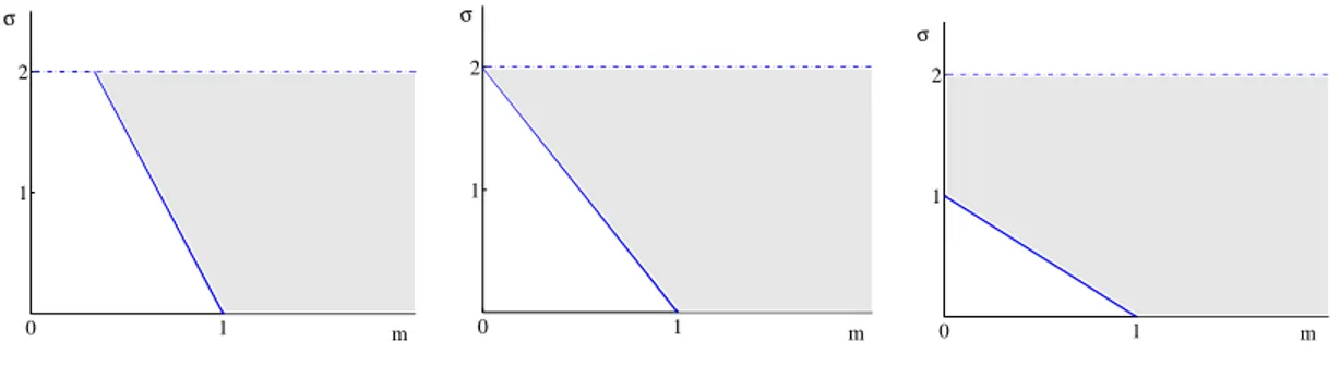
As in the case of the PME, there is a unified theory of existence and uniqueness of a suitable concept of weak solution above a critical exponent, given for a general σ ∈(0,2) by m∗ ≡(N −σ)+/N. The linear casem = 1 lies always in this range.
Theorem 2.1 Let m > m∗ and σ ∈ (0,2). For every f ∈ L1(RN) there exists a
1 0
1 2
m
σ
0 1
1 2
m
σ
0 1
1 2
m
σ
Figure 1: The critical line m∗ = (N −σ)/N and the supercritical region m > m∗ for
N ≥3,N = 2, and N = 1.
The precise definition of weak solution that guarantees uniqueness is stated in Def-inition 3.1 or equivalently in DefDef-inition 3.2.
The construction of the solution in the previous theorem follows from a double limit procedure, approximating first the initial datum by a sequence of bounded functions, and also approximating RN by a sequence of bounded domains with null boundary data. In this respect we show existence of a weak solution to the associated Cauchy-Dirichlet problem, a result that has an independent interest, see Section 4.
The weak solutions to Problem (1.1) have some nice qualitative properties that are summarized as follows.
Theorem 2.2 Assume the hypotheses of Theorem2.1, and letube the weak solution to Problem (1.1).
(i) ∂tu∈L∞((τ,∞) :L1(RN)) for every τ >0. (ii) Mass is conserved: RRNu(x, t)dx=
R
RNf(x)dx for all t≥0.
(iii) Let u1, u2 be the weak solutions to Problem (1.1) with initial data f1, f2 ∈
L1(RN). Then, Z
RN
(u1−u2)+(x, t)dx≤
Z
RN
(f1−f2)+(x)dx, (L1-order-contraction property).
(iv) Any Lp-norm of the solution, 1≤p≤ ∞, is non-increasing in time.
(v) The solution is bounded in RN × [τ,∞) for every τ > 0 (L1-L∞ smoothing
effect). Moreover, for all p≥1,
(2.1) ku(·, t)kL∞(
RN) ≤C t−γpkfkδp
Lp(RN),
(vii) If either m ≥1 or f ≥0, then u∈Cα(RN ×(0,∞)) for some 0< α <1. (viii) The solution depends continuously on the parameters σ ∈ (0,2), m > m∗, and
f ∈L1(RN) in the norm of the space C([0,∞) : L1(RN)).
Remarks. (a) Properties (i) and (ii) were only known for σ = 1 in the case of nonnegative initial data [35].
(b) The positivity property (vi) is not true for the PME in the range m > 1. The fact that it holds for Problem (1.1) stems from the nonlocal character of the diffusion operator.
(c) A weak solution satisfying property (i) is said to be astrong solution, see Defini-tion 6.1. These kind of soluDefini-tions satisfy the equaDefini-tion in (1.1) almost everywhere in Q=RN ×(0,∞).
Our main interest in this paper is in describing the theory in the above mentioned range m > m∗. However, we also consider the lower range 0< m ≤m∗ for contrast.
In that range (which implies that 0 < σ < 1 if N = 1) we obtain existence if we restrict the data class (or if we relax the concept of solution). In addition, in order to have uniqueness, we need to ask the solution to be strong.
Theorem 2.3 Let σ ∈ (0,2) and 0 < m ≤ m∗. For every f ∈ L1(RN)∩Lp(RN)
with p > p∗(m) = (1−m)N/σ there exists a unique strong solution to Problem (1.1).
0 1
1
m p
m
*
N/σ
Figure 2: The critical line p∗ = (1 −m)N/σ and the existence region of strong
solutions.
This theorem improves the results obtained of [35] for σ = 1, since in that paper existence and uniqueness of a (weak) solution were only proved for the case of inte-grable and bounded initial data,f ∈L1(RN)∩L∞(RN). Moreover, the weak solution was only proved to be strong in the case of nonnegative initial data.
Theorem 2.4 Assume the hypotheses of Theorem 2.3, and letu be the strong solu-tion to Problem (1.1).
(i) The mass RRNu(x, t)dx is conserved if m = m∗. Mass is not conserved if
m < m∗. Actually, when 0 < m < m∗ there is a finite time T > 0 such that
u(x, T)≡0 in RN.
(ii) There is an L1-order-contraction property.
(iii) Any Lp-norm of the solution, 1≤p≤ ∞, is non-increasing in time.
(iv) The solution is bounded in RN ×[τ,∞) for every τ > 0 (Lp-L∞ smoothing
effect). Moreover, if p > p∗(m) (which is necessary to make γp > 0) then
formula (2.1) holds.
(v) If f ≥0 the solution is positive for all x and all positive times up to the extinc-tion time.
(vi) Let f ≥0and let T be the extinction time. Then u∈Cα(RN×(0, T))for some 0< α <1.
We will make a series of comments on these two results. First, we point out that the result on the conservation of mass for m=m∗ is new even for σ= 1.
A more essential observation is that there is an alternative approach: using the results of Crandall and Pierre [22] we can obtain the existence of a unique so-called
mild solution for all f ∈ L1(RN) in the whole range of m and σ, via the abstract theory of accretive operators. This approach has therefore the advantage of having general scope. Two problems arise with this way of looking at the problem: (a) how to characterize the mild solution in differential terms; and (b) how to derive its properties. Our paper answers both questions.
The strong solutions that we have constructed are mild solutions. Hence, in our restricted range of initial data the unique mild solution is a strong solution. For a general f ∈L1(RN) and m ≤m
∗, we will show that the mild solution is a very weak
solution (a solution in the sense of distributions), see Theorem 8.4. However, we will fail to prove that this very weak solution is a weak solution in the sense of Definition 3.1, and hence we will not be able to obtain the properties listed above (bit note that the L1-contraction holds since it is a consequence of the accretivity of the operator).
As to the continuous dependence of the solution in terms of the parameters, conver-gence inL1(RN) is not expected to hold for 0 < m < m
∗, since mass is not conserved
in that region. Instead we expect to have continuity in weighted spaces, much in the spirit of [5]. Nevertheless, we are able to extend the continuous dependence result of Theorem 2.2-(viii) to cover the casem =m∗ forN >2, see Proposition 10.1. We also
3
Weak solutions. An equivalent problem
3.1
Weak solutions
If ψ and ϕ belong to the Schwartz class, Definition (1.2) of the fractional Laplacian together with Plancherel’s theorem yield
(3.1)Z
RN
(−∆)σ/2ψ ϕ= Z
RN|
ξ|σψˆϕˆ= Z
RN|
ξ|σ/2ψˆ|ξ|σ/2ϕˆ= Z
RN
(−∆)σ/4ψ(−∆)σ/4ϕ. Therefore, if we multiply the equation in (1.1) by a test function ϕ and integrate by parts, as usual, we obtain
(3.2)
Z ∞
0
Z
RN
u∂ϕ
∂t dxds− Z ∞
0
Z
RN
(−∆)σ/4(|u|m−1u)(−∆)σ/4ϕ dxds= 0. This identity will be the basis of our definition of a weak solution.
The integrals in (3.2) make sense if u and |u|m−1u belong to suitable spaces. The
correct space for |u|m−1u is the fractional Sobolev space ˙Hσ/2(RN), defined as the completion of C∞
0 (RN) with the norm kψkH˙σ/2 =
Z
RN|
ξ|σ|ψˆ|2dξ
1/2
=k(−∆)σ/4ψk2.
Definition 3.1 A function u is a weak (L1-energy solution) to Problem (1.1) if:
• u∈C([0,∞) :L1(
RN)), |u|m−1u∈L2
loc((0,∞) : ˙Hσ/2(RN)); • identity (3.2) holds for every ϕ ∈C1
0(RN ×(0,∞)); • u(·,0) =f almost everywhere.
For brevity we will call weak solutions the solutions obtained below according to this definition, but the complete name weak L1-energy solution is used in the statement
to recall that we are making a very definite choice.
The main disadvantage in using this definition is that there is no formula for the fractional Laplacian of a product, or of a composition of functions. Moreover, there is no benefit in using compactly supported test functions since their fractional Laplacian loses this property. To overcome these difficulties, we will use the fact that our solution u is the trace of the solution of a local problem obtained by extending |u|m−1u to a
half-space whose boundary is our original space.
3.2
Extension Method
Ifg =g(x) is a smooth bounded function defined inRN, its σ-harmonic extension to the upper half-space,v = E(g), is the unique smooth bounded solution v =v(x, y) to
(3.3)
∇ ·(y1−σ∇v) = 0, inRN+1
+ ≡ {(x, y)∈RN+1 :x∈RN, y >0},
Then, Caffarelli and Silvestre [13] proved that
(3.4) −µσ lim y→0+y
1−σ∂v
∂y = (−∆)
σ/2g(x), µσ = 2σ−1Γ(σ/2)/Γ(1
−σ/2).
In (3.3) the operator ∇ acts in all (x, y) variables, while in (3.4) (−∆)σ/2 acts only
on the x= (x1,· · · , xN) variables. In the sequel we denote
Lσv ≡ ∇ ·(y1−σ∇v), ∂v
∂yσ ≡µσylim→0+y
1−σ∂v ∂y.
Operators like Lσ, with a coefficient y1−σ, which belongs to the Muckenhoupt space of weights A2 if 0 < σ <2, have been studied by Fabes et al. in [24]. We make use of
this theory later in the proof of positivity, see Theorem 9.1.
With the above in mind, we rewrite Problem (1.1) as a quasi-stationary problem for w= E(|u|m−1u) with a dynamical boundary condition
(3.5)
Lσw= 0, (x, y)∈RN++1, t >0,
∂w ∂yσ −
∂|w|m1−1w
∂t = 0, x∈R
N, y = 0, t >0, w=|f|m−1f, x∈RN, y = 0, t= 0.
To define a weak solution of this problem we multiply formally the equation in (3.5) by a test function ϕ and integrate by parts to obtain
(3.6)
Z ∞
0
Z
RN
u∂ϕ
∂t dxds−µσ Z ∞
0
Z
RN++1
y1−σh∇w,∇ϕidxdyds= 0,
where u =|Tr(w)|m1−1Tr(w). This holds on the condition that ϕ vanishes for t = 0
and also for large |x|, y and t. We then introduce the energy space Xσ(RN+1 + ), the
completion of C∞
0 (RN++1) with the norm
(3.7) kvkXσ = µσ
Z
RN++1
y1−σ|∇v|2dxdy !1/2
.
The trace operator is well defined in this space, see below.
Definition 3.2 A pair of functions (u, w) is a weak solution to Problem (3.5) if:
• u=|Tr(w)|m1−1Tr(w)∈C([0,∞) :L1(RN)), w∈L2
loc((0,∞) : Xσ(RN++1)); • identity (3.6) holds for every ϕ ∈C1
0
RN++1×(0,∞)
;
For brevity we will refer sometimes to the solution as onlyu, or even onlyw, when no confusion arises, since it is clear how to complete the pair from one of the components, u=|Tr(w)|m1−1Tr(w),w= E(|u|m−1u).
The extension operator is well defined in ˙Hσ/2(
RN). It has an explicit expression using aσ-Poisson kernel, and E : ˙Hσ/2(RN)→Xσ(RN+1
+ ) is an isometry, see [13]. The
trace operator, Tr : Xσ(RN+1
+ ) → H˙σ/2(RN) is surjective and continuous. Actually,
we have the trace embedding
(3.8) kΦkXσ ≥ kE(Tr(Φ))kXσ =kTr(Φ)k˙
Hσ/2
for any Φ∈Xσ(RN).
3.3
Equivalence of the weak formulations
The key point of the above discussion is that the definitions of weak solution for our original nonlocal problem and for the extended local problem are equivalent. Thus, in the sequel we will switch from one formulation to the other whenever this may offer some advantage.
Proposition 3.1 A function u is a weak solution to Problem (1.1) if and only if
(u,E(|u|m−1u)) is a weak solution to Problem (3.5).
Since E : ˙Hσ/2(RN)→Xσ(RN+1
+ ) is an isometry, we have
µσ Z
RN++1
y1−σh∇E(ψ),∇E(ϕ)i= Z
RN
(−∆)σ/4ψ(−∆)σ/4ϕ,
for every ψ, ϕ ∈ H˙σ/2(
RN). Hence the result follows immediately from the next lemma, which states that any σ-harmonic function is orthogonal in Xσ(RN+1
+ ) to
every function with trace 0 on RN. Lemma 3.1 Letψ ∈H˙σ/2(RN)andΦ
1,Φ2 ∈Xσ(R+N+1)such thatTr(Φ1) = Tr(Φ2).
Then
µσ Z
RN++1
y1−σh∇E(ψ),∇Φ1i=µσ Z
RN++1
y1−σh∇E(ψ),∇Φ2i.
Proof. Leth = Φ1−Φ2. Since E(ψ) is smooth for y >0, given ε >0 we have, after
integrating by parts,
µσ Z ∞
ε Z
RN
y1−σh∇E(ψ),∇hidxdy =µσ Z
RN
ε1−σ∂E(ψ)
∂y (x, ε)h(x, ε)dx.
The left-hand side converges toµσRRN+1
+ y
4
The problem in a bounded domain
As an intermediate step in the development of the theory for Problem (1.1), we will also consider the Cauchy-Dirichlet problem associated to the fractional PME,
(4.1)
∂u
∂t + (−∆)
σ/2(|u|m−1u) = 0, x∈Ω, t >0,
u= 0, x∈∂Ω, t >0,
u(x,0) =f(x), x∈Ω,
where Ω⊂RN is a smooth bounded domain,f ∈L1(Ω). This problem has an interest
in itself.
Let us present here the main facts and results about this problem. In view of formula (1.4), the fractional operator (−∆)σ/2 in a bounded domain can be described
in terms of a spectral decomposition. Let{ϕk, λk}∞
k=1 denote an orthonormal basis of
L2(Ω) consisting of eigenfunctions of −∆ in Ω with homogeneous Dirichlet boundary
conditions and their corresponding eigenvalues. The operator (−∆)σ/2 is defined for
any u∈C∞
0 (Ω), u=
P∞
k=1ukϕk, by
(−∆)σ/2u=
∞
X
k=1
λσ/k 2ukϕk.
This operator can be extended by density foru in the Hilbert space
H0σ/2(Ω) ={u∈L2(Ω) :kuk2 H0σ/2 =
∞
X
k=1
λσ/k 2u2k <∞}.
Definition 4.1 A function u is a weak solution to Problem (4.1) if:
• u∈C([0,∞) :L1(Ω)), |u|m−1u∈L2
loc((0,∞) :H
σ/2 0 (Ω)); • Identity
Z T
0
Z
Ω
u∂ϕ
∂t dxds− Z T
0
Z
Ω
(−∆)σ/4um(−∆)σ/4ϕ dxds= 0
holds for every ϕ ∈C1
0(Ω×(0, T)); • u(·,0) =f almost everywhere in Ω.
The hypotheses that we need in order to have existence when the spatial domain is bounded coincide with the ones we have when the spatial domain is the whole RN.
Theorem 4.1 Problem (4.1) has a unique weak solution ifm > m∗ and f ∈L1(Ω),
which is moreover strong, and a unique strong solution if m ≤ m∗ and f ∈ Lp(Ω)
As for the properties of the solutions, most of them, though not all, coincide with the ones that hold when the domain is the whole space.
Theorem 4.2 Assume the hypotheses of Theorem 4.1, and let u be the strong solu-tion to Problem (4.1).
(i) The solution is bounded in Ω×[τ,∞) for every τ > 0. Moreover, a formula analogous to (2.1) holds.
(ii) As a consequence, RΩu(x, t)dx = O(t−γp). Moreover, if 0 < m < 1 there is
extinction in finite time.
(iii) There is an L1-order-contraction property.
(iv) Any Lp-norm of the solution, 1≤p≤ ∞, is non-increasing in time.
(v) The solution depends continuously on the parameters σ ∈ (0,2), m > m∗, and
f ∈L1(Ω) in the norm of the space C([0,∞) : L1(Ω)).
The results of [3] imply that u∈Cα for m≥1. Positivity for any m > 0 when the initial data are nonnegative, and Cα regularity for m <1 are still open problems.
The construction of a solution uses the analogous to the Caffarelli-Silvestre exten-sion (3.3), restricted here to the upper half-cylinder CΩ = Ω× (0,∞), with null
condition on the lateral boundary, ∂Ω ×(0,∞), a construction considered in [12], [38], [10], [16]. Thus, w= E(|u|m−1u) satisfies
(4.2)
Lσw= 0, (x, y)∈CΩ, t >0,
w= 0, x∈∂Ω, y >0, t >0, ∂w
∂yσ −
∂|w|m1−1w
∂t = 0, x∈Ω, y = 0, t >0, w=|f|m−1f, x∈Ω, y = 0, t= 0.
In order to define a weak solution to (4.2) we need to consider the space Xσ
0(CΩ),
the closure of C∞
c (CΩ) with respect to the norm (3.7), withRN++1 substituted by CΩ.
The extension and trace operators between H0σ/2(Ω) and Xσ
0(CΩ) satisfy the same
properties as in the case of the whole space. In fact
µσ Z
CΩ
y1−σ|∇E(ϕ)|2 1/2
=kE(ϕ)kXσ
0 =kϕkH0σ/2
=k(−∆)σ/4ϕk
2 =P∞k=1λσ/k 2ϕ2k 1/2
.
See for instance [10] for the explicit expression of E(ϕ) in terms of the coefficients ϕk.
Definition 4.2 A pair of functions (u, w) is a weak solution to Problem (4.2) if:
• u=|Tr(w)|m1−1Tr(w)∈C([0,∞) :L1(Ω)), w∈L2
• identity
Z ∞
0
Z
Ω
u∂ϕ
∂t dxds−µσ Z ∞
0
Z
CΩ
y1−σh∇w,∇ϕidxdyds= 0,
holds for every ϕ =ϕ(x, y, t) such that ϕ∈C1
0(Ω×[0,∞)×(0,∞)); • u(·,0) =f almost everywhere in Ω.
As it happens for the case where Ω = RN, the two definitions of weak solution, Definitions 4.1 and 4.2, are equivalent.
Remark. The space H0σ/2(Ω) can also be defined by interpolation, see [32]. We notice that, though for 1< σ <2 the solutions are zero almost everywhere at the boundary, for 0 < σ ≤ 1 the functions in H0σ/2(Ω) do not have a trace, [32]. Therefore, the boundary condition must be understood in a weak sense, see also [12] for the case σ = 1.
5
Some functional inequalities
In this section we gather some functional inequalities related with the fractional Lapla-cian, both in the whole space or in a bounded domain, that will play an important role in the sequel. The first one, Strook-Varopoulos’ inequality, is well known in the theory of sub-Markovian operators [33]. Nevertheless, we give a very short proof using the extension operator that makes apparent the power of this technique.
Lemma 5.1 (Strook-Varopoulos’ inequality) Let 0< γ < 2, q >1. Then
(5.1)
Z
RN
(|v|q−2v)(−∆)γ/2v ≥ 4(q−1) q2
Z
RN
(−∆)γ/4|v|q/22
for all v ∈Lq(RN) such that (−∆)γ/2v ∈Lq(RN). Proof. Using property (3.1) and Lemma 3.1, we get
Z
RN
(|v|q−2v)(−∆)γ/2v = Z
RN
(−∆)γ/4(|v|q−2v)(−∆)γ/4v
= µγ Z
RN++1
y1−γh∇(|E(v)|q−2E(v)),∇E(v)i
= µγ4(q−1) q2
Z
RN++1
y1−γ|∇(|E(v)|q/2)|2
≥ 4(q−1)
q2
Z
RN
(−∆)γ/4|v|q/22.
In the last step we get only inequality because the function|E(v)|q/2 is not necessarily
γ-harmonic.
Lemma 5.2 Let 0< γ <2. Then
(5.2)
Z
RN
ψ(v)(−∆)γ/2v ≥ Z
RN
(−∆)γ/4Ψ(v)2
whenever ψ′ = (Ψ′)2.
Proof. Use the extension method and the property h∇ψ(w),∇wi=|∇Ψ(w)|2.
In order to prove our second inequality we need the well-known Hardy-Littlewood-Sobolev’s inequality [25], [37], [31]: for every v such that (−∆)γ/2v ∈ Lr(RN), 1 < r < N/γ, 0< γ <2, it holds
(5.3) kvkr1 ≤c(N, r, γ)k(−∆)
γ/2v kr,
r1 = NN r−γr. Putting for instancer= 2,γ =σ/2, we obtain the inclusion ˙Hσ/2(RN)֒→
LN2−Nσ(RN) whenever N > σ. What happens for N = 1≤σ < 2? Or more generally,
for r≥N/γ? We answer this question in the next lemma.
Lemma 5.3 (Nash-Gagliardo-Nirenberg type inequality) Let p ≥ 1, r > 1,
0 < γ < min{N,2}. There is a constant C = C(p, r, γ, N) > 0 such that for any
v ∈Lp(RN) with (−∆)γ/2v ∈Lr(RN) we have
(5.4) kvkαr2+1≤Ck(−∆)γ/2vkrkvkαp ,
where r2 = Nr(rp(N+−rγ−)p), α = p(rr−1).
Proof. We use (5.1). Estimate now the left hand side of this inequality using inequality (5.3), and the right hand side with H¨older’s inequality, to get (5.4).
Notice that, for r = 2 and γ = σ/2, this corresponds to using inequality (5.3) for the space ˙Hσ/4(RN) instead of ˙Hσ/2(RN), thus allowing all values of σ ∈(0,2) even in the case N = 1.
Inequalities of this kind are already available [8]. However, this particular one is, up to our knowledge, new. Let us explain in more detail the consequences of this inequality in relation to (5.3).
Assume first that N > γr. Hardy-Littlewood-Sobolev’s inequality (5.3) implies that if (−∆)γ/2v ∈ Lr then v ∈ Lr1. Assuming also v ∈ Lp, then (5.4) gives that
v ∈ Lr1 ∩Lr2, which is always stronger that v ∈ Lr1 ∩Lp. Both results coincide in
the case p=r1 =r2.
If on the contrary N ≤ γr, we cannot apply Hardy-Littlewood-Sobolev, but (5.4) gives that v ∈Lp∩Lr2.
We now consider the case of a bounded domain Ω ⊂ RN. The characterization of the fractional Laplacian in terms of the extension to the half-cylinderCΩ allows us to
Lemma 5.4 Strook-Varopoulos’ inequalities (5.1)and (5.2) hold true with RN sub-stituted by Ω⊂RN bounded.
On the other hand, let v ∈H0σ/2(Ω). Consider its σ-extension w= E(v), (σ = 2γ), and let we be the extension of w by zero outside the half-cylinder. Then we have the estimate, see [10], [19],
µσ Z
RN++1
y1−σ|∇we|2 ≥S(σ, N) Z
RN|
Tr(w)e |N2−Nσ
N−σ
N
.
i.e.,
(5.5) µσ Z
Ω
y1−σ|∇w|2 ≥S(σ, N) Z
Γ|
v|N2−Nσ
N−σ
N
.
The left hand side equalsk(−∆)γ/2vk2
2. That is, we have obtained inequality (5.3) in
the case r = 2.
From this point, we can repeat the proof of Lemma 5.3, which only uses the case just proved and H¨older’s inequality, thus obtaining inequality (5.4) also for a bounded domain.
More important is the following application.
Lemma 5.5 (Sobolev type inequality) Let Ω ⊂ RN be a bounded domain, and let v be such that (−∆)γ/2v ∈Lr(Ω), N ≥1, 0< γ < 2. Then we have
(5.6) kvkq ≤C(q, r, N, γ)k(−∆)γ/2vkr
for every 1≤q ≤ N r
N−γr if N > γr, or for every q≥1 if γ < N ≤γr.
Proof. If N > γr we just apply (5.4) with p= NN r−γr, and apply H¨older’s inequality for the exponents 1 ≤ q < N r
N−γr. If γ < N ≤ γr, and given any q > N N−γ, we apply (5.4), this time with s= NN q+γq < N
γ ≤r instead of r, and p=q. We end again with H¨older’s inequality for the exponents 1≤q≤ NN−γ.
6
Uniqueness
In this section we prove the uniqueness parts of Theorems 2.1 and 2.3.
Notations. We will use the simplified notation um for data of any sign, instead of the actual “odd power” |u|m−1u. In the same way, w1/m will stand for |w|m1−1w. In
6.1
m > m
∗. Uniqueness of weak solutions
Theorem 6.1 Let f ∈ L1(RN) and m > m
∗. Problem (1.1) has at most one weak
solution.
Proof. We adapt the classical uniqueness proof due to Oleinik [34]. This will require u∈Lm+1(RN×(0, T)), which will be true ifm > m
∗. To prove this we apply H¨older’s
inequality twice, first in space and then in time, using inequality (5.3). Assume first N > σ. We have
Z T
0
Z
RN|
u|m+1dxdt≤ Z T
0
Z
RN|
u|dxβ( Z
RN |
u|2NNm−σ dx
1−β dt
≤CTRN max
t∈[0,T]ku(·, t)k
β
1
h Z T
0
Z
RN|
u|2NNm−σ dx
N−σ
N
dti1−γ,
where β = N(Nm(2−m1)+−σ1)+(mσ+1) and γ = NN(2(mm−−1)+1)+σσ. Observe that m > m∗ implies β, γ ∈
(0,1). Applying now inequality (5.3), we get Z T
0
Z
RN|
u|m+1dxdt≤Ch Z T
0 k
um(·, t)k2H˙σ/2dt
i1−γ
≤C.
In the case N = 1 and 1≤σ <2 the computation is similar. But we have to use the Nash-Gagliardo-Nirenberg type inequality (5.4) instead to get the same conclusion. What we get in this case is
Z T
0
Z
RN|
u|m+1dxdt≤ Z T
0
Z
RN|
u|dx
δ γ
dt
γZ T
0
Z
RN|
u|22m−+1σ dx
2−σ dt
1−γ
≤CTγ max
t∈[0,T]ku(·, t)k
δ+1−γ
1
Z T
0 k
um(·, t)k2H˙σ/2dt
1−γ
≤C,
where now δ = σ2(mm−+1)1+−σ1 and γ = 2mm−−1+1+σσ.
We now proceed with the core of the proof. Let u and eu be two weak solutions to Problem (1.1). We take the following function as test in the weak formulation
ϕ(x, t) = Z T
t
(um−uem)(x, s)ds, 0≤t≤T, with ϕ ≡0 for t≥T. We have
Z T
0
Z
RN
(u−eu)(x, t)(um−uem)(x, t)dxdt
+ Z T
0
Z
RN
(−∆)σ/4(um−uem)(x, t) Z T
t
(−∆)σ/4(um−eum)(x, s)ds dxdt= 0. Integration of the second term gives
Z T
0
Z
RN
(u−eu)(x, t)(um−uem)(x, t)dxdt
+1 2 Z RN Z T 0
(−∆)σ/4(um−uem)(x, s)ds 2
Since both integrands are nonnegative, they must be identically zero. Therefore,
u=eu.
Remark. The same proof works without any restriction on the exponent m provided u∈Lm+1(RN ×(τ, T)).
6.2
m
≤
m
∗. Uniqueness of strong solutions
Weak solutions satisfy the equation in (1.1) in the sense of distributions. Hence, if the left hand side is a function, the right hand side is also a function and the equation holds almost everywhere. This fact allows to prove several important properties, among them uniqueness for m≤m∗, and hence motivates the following definition.
Definition 6.1 We say that a weak solutionu to Problem (1.1)is a strong solution if ∂tu∈L∞((τ,∞) :L1(RN)), for every τ > 0.
In the case of strong solutions the uniqueness result also provides a comparison principle. The following uniqueness proof is valid for all values of m >0.
Theorem 6.2 Let m > 0. If u1, u2, are strong solutions to Problem (1.1) with
initial data f1, f2 ∈L1(RN), then, for every 0≤t1 < t2 it holds
(6.1)
Z
RN
(u1−u2)+(x, t2)dx≤
Z
RN
(u1−u2)+(x, t1)dx.
Proof. Letp∈ C1(R)∩L∞(R) be such that p(s) = 0 for s ≤0, p′(s)> 0 fors > 0
and 0 ≤ p ≤ 1, and let j be such that j′ = √p′, j(0) = 0. We will choose p as an
approximation to the sign function.
Let us first assume that t1 >0. We subtract the equations satisfied by u1 and u2,
multiply by the function ϕ=p(um
1 −um2 ), and integrate by parts to get
Z t2
t1
Z
RN
∂(u1−u2)
∂t p(u m
1 −um2 ) =−
Z t2
t1
Z
RN
(−∆)σ/2(um1 −um2 )p(um1 −um2 ).
We now apply the generalized Strook-Varopoulos inequality (5.2), to get Z t2
t1
Z
RN
∂(u1−u2)
∂t p(u m
1 −um2 )≤ −C
Z t2
t1
Z
RN|
(−∆)σ/4j(um1 −um2 )|2 ≤0.
We end by letting ptend to the sign function. The case t1 = 0 is obtained passing to
the limit.
7
Existence for bounded initial data
Crandall and Pierre developed in [22] an abstract approach to study evolution equa-tions of the form∂tu+Aϕ(u) = 0 whenAis an m-accretive operator inL1 and ϕis a
monotone increasing real function. This allows to obtain a so-calledmild solution us-ing Crandall-Liggett’s Theorem. Our problem falls within this framework. However, such an abstract construction does not give enough information to prove that the mild solution is in fact a weak solution, in other words, to identify the solutions in a differential sense. We will use an alternative approach to construct the mild solution whose main advantage is precisely that it provides enough estimates to show that it is a weak solution, and later that it is strong.
In order to develop the theory for Problem (1.1), we will approximate the initial data f by a sequence fn∈ L1(RN)∩L∞(RN), and use a contraction property in order to pass to the limit. Hence, our first task is to obtain existence for integrable, bounded initial data. This is the goal of the present section
We will construct solutions by means of Crandall-Liggett’s Theorem [21], which is based on an implicit in time discretization. Hence, we will have to deal with the elliptic problem
(7.1)
Lσw= 0 inRN++1, −∂y∂wσ +w
1/m=g onRN.
Equalities on RN have to be understood in the sense of traces. To show existence of a weak solution for this problem we approximate the domain RN++1 by half-cylinders,
BR×(0,∞), with zero data at the lateral boundary, ∂BR×(0,∞). We recall that in the case σ = 1 a similar construction is performed in [35], though there half-balls were used instead of half-cylinders.
Now we have two choices: either we first pass to the limit in the discretization, to obtain a solution of the parabolic problem in the ball BR, and then pass to the limit R → ∞; or we first pass to the limit in R to obtain a solution of the elliptic problem in the whole space and then pass to limit in the discretization. We will follow both approaches (each of them has its own advantages) and will later prove that both of them produce the same solution.
Instead of just considering problems in balls we will analyze the case of any bounded open domain Ω⊂RN, since it has independent interest.
7.1
Problem in a bounded domain
In order to check that the hypotheses of Crandall-Liggett’s theorem hold, we have to prove existence of a weak solution w of (7.1) (defined in the standard way) and contractivity of the mapg 7→w1/m(·,0) in the norm ofL1(Ω) for the elliptic problem
Theorem 7.1 Let Ω⊂RN be a bounded domain. For everyg ∈L∞(Ω) there exists
a unique weak solutionw∈ Xσ
0(CΩ)to Problem (7.1). It satisfieskw(·,0)k∞≤ kgkm∞.
Moreover, there is a T-contraction property in L1: if w and we are the solutions
corresponding to data g and eg, then
(7.2)
Z
Ω
w1/m(x,0)−we1/m(x,0)+ dx≤ Z
Ω
[g(x)−eg(x)]+ dx.
Proof. The existence of a weak solution, i.e., a function w∈Xσ
0(CΩ) satisfying
(7.3) µσ Z
CΩ
y1−σh∇w,∇ϕi+ Z
Ω
v1/mϕ− Z
Ω
gϕ= 0,
v = Tr(w), for every test function ϕ, is obtained in a standard way by minimizing the functional
J(w) = µσ 2
Z
CΩ
y1−σ|∇w|2+ m
m+ 1 Z
Ω|
v|mm+1 −
Z
Ω
vg.
This functional is coercive in Xσ
0(CΩ). Indeed, the first term kwk2Xσ
0, and is using
H¨older’s inequality, we have Z Ω vg
≤ kvk 2N N−σ kgk
2N
N+σ ≤εkvk
2
2N
N−σ
+ 1 εkgk
2
2N
N+σ.
Now, the trace embedding (5.5) implies
(7.4) J(w)≥C1kwk2Xσ
0 −C2.
For N = 1 ≤ σ < 2 we use inequality (5.6) instead. In fact, putting q = r = 2, γ =σ/2, we get kwkXσ
0 ≥Ckvk2. We obtain again (7.4).
We now establish contractivity of solutions to Problem (7.1) inL1(Ω). Let wand
e w be the solutions corresponding to datag andeg. If we consider in the weak formulation the test function ϕ = p(w−w), wheree p is any smooth monotone approximation of the sign function, 0≤p(s)≤1, p′(s)≥0, we get
µσ Z
CΩ
y1−σp′(w−w)e |∇(w−w)e |2+ Z
Ω
(w1/m−we1/m)p(w−w)e − Z
Ω
(g−g)e p(w−w) = 0.e
Passing to the limit, we obtain Z
Ω
(w1/m−we1/m)+ ≤
Z
Ω
(g−eg) sign(w−w)e ≤ Z
Ω
(g−eg)+.
In particular, under the assumption g ≥0 we have w(·,0)≥0. Standard comparison gives noww≥0 inCΩ. In the same way we can establish a contractivity property for
subsolutions and supersolutions to the problem with nontrivial, on Ω×(0,∞), bound-ary condition. We thus may take the constant function eg =kgk∞as a supersolution,
to get kw1/mk
∞ ≤ kgk∞. We also deduce the estimate
(7.5) µσ
Z
CΩ
y1−σ|∇w|2 ≤ Z
Ω
We now construct a solution to the parabolic problem in the bounded domain.
Theorem 7.2 Let Ω ⊂ RN bounded. For every f ∈ L∞(Ω) there exists a weak
solution (u, w) to Problem (3.5) with u(·, t) ∈ L∞(Ω) for every t > 0 and w ∈
L2([0, T];Xσ
0(CΩ)). Moreover, the following contractivity property holds: if (u, w),
(eu,w)e are the constructed weak solutions corresponding to initial data f, fe, then
(7.6)
Z
Ω
[u(x, t)−u(x, t)]e +dx≤
Z
Ω
[f(x)−f(x)]e +dx.
In particular a comparison principle for constructed solutions is obtained.
Proof. Crandall-Liggett’s result only provides us in principle with an abstract type of solution calledmild solution. However, we know that (7.3) and (7.5) hold, from where it is standard to show that the mild solution is in fact weak, see for example [35]. We recall the main idea: For each time T > 0 we divide the time interval [0, T] in n subintervals. Letting ε = T /n, we construct the pair function (uε, wε) piecewise constant in each interval (tk−1, tk], where tk = kε, k = 1,· · · , n, as the solutions to
the discretized problems
Lσwε,k = 0 in CΩ,
ε∂wε,k ∂yσ =w
1/m
ε,k −uε,k−1 on Ω,
with uε,k−1 = wε,k1/m−1(·,0), uε,0 =f. The mild solution is obtained by letting ε → 0.
We still have to check that it is a weak solution.
Crandall-Ligget’s Theorem gives that uε converges in L1(Ω) to some function u ∈ C([0,∞) : L1(Ω)). Moreover, kwεk
∞ ≤ kfkm∞. Hence, wε converges in the weak-∗
topology to some function w∈L∞(C
Ω×[0,∞]). On the other hand, multiplying the
equation by wε,k, integrating by parts, and applying Young’s inequality, we obtain
1 (m+ 1)
Z
Ω|
uε(x, t)|m+1dx+µσ Z T
0
Z
CΩ
y1−σ|∇wε(x, t)|2dxdydt
≤ (m1+ 1)
Z
Ω|
f(x)|m+1dx.
Passing to the limit, the following estimate is obtained for the weighted norm of|∇w|,
µσ Z T
0
Z
CΩ
y1−σ|∇w(x, t)|2dxdydt≤ 1 (m+ 1)
Z
Ω|
f(x)|m+1dx,
and therefore w ∈ L2([0, T];Xσ
0(CΩ)). Now, choosing appropriate test functions, as
in [35], it follows that we can pass to the limit in the elliptic weak formulation to get the identity of the parabolic weak formulation.
7.2
The problem in the whole space
Theorem 7.3 For every f ∈L1(RN)∩L∞(RN) there exists a weak solution (u, w)
to Problem (3.5). This solution satisfies u(·, t)∈L1(RN)∩L∞(RN) for every t > 0,
and w∈L2([0, T] :Xσ(RN+1
+ )). Moreover, the following contractivity property holds:
if (u, w), (eu,w)e are the constructed weak solutions corresponding to initial data f, fe, then
(7.7)
Z
RN
[u(x, t)−u(x, t)]e +dx≤
Z
RN
[f(x)−fe(x)]+dx.
In particular a comparison principle for constructed solutions is obtained.
Proof. Let us comment briefly the two constructions of the solution.
Take to begin with as domain Ω =BR, the ball of radiusRcentered at the origin, and let wR(fR) be the corresponding solution to problem (7.1) with datum fR=f·χBR.
Passing to the limitR→ ∞we obtain a weak solutionwto the elliptic problem in the upper half-space RN++1. Now we can follow the technique described above using the
time discretization scheme thus obtaining a weak solution, whose trace on{y= 0}we call U =U(f). This is the mild solution produced by the Crandall-Liggett theorem and as such is unique. The contractivity property (7.7) follows from (7.6).
As to the second construction, we use the weak solution uR(fR) to the parabolic problem posed in the ballBR, as obtained in Theorem 7.2. In the study of this limit we first treat the case where f ≥ 0 and fR approximates f from below. Then, the family of solutions uR(fR) is monotone in R and also uR(fR) ≤ U(f) follows from simple comparison. In this way we ensure the existence of
e
u(x, t) = lim
R→∞uR(x, t)
It is easy to prove that euis also a weak solution with initial dataf and u(f)e ≤U(f). The equivalence of the two solutions depends on the already proved uniqueness result, see the remark after Theorem 6.1.
In the general case where f changes sign, we use comparison with the construction for f+ and f− to show that the family uR(f) is bounded uniformly and then use
compactness to pass to the limit and obtain a weak solution. Again we end by
checking that eu=U.
Remark. Since we have uniqueness, as a byproduct of the limit processes of con-struction we get the following estimates for weak solutions with initial data f ∈ L1(RN)∩L∞(RN):
ku(·, t)k1 ≤ kfk1, ku(·, t)k∞≤ kfk∞.
Remark. In the course of the proof we have obtained a unique weak solution to the nonlocal nonlinear elliptic problem
for every g ∈ L1(Ω)∩L∞(Ω), both for Ω = RN and for Ω a bounded domain with homogeneous Dirichlet condition. This weak solution satisfies u∈L1(Ω)∩L∞(Ω).
8
Existence for general data
We prove here existence for data f ∈L1(
RN). The idea is to approximate the initial data by a sequence of bounded integrable functions and then pass to the limit in the approximate problems. The key tools needed to pass to the limit are the L1
-contraction property and the smoothing effect. As a preliminary step we must show that the approximate solutions are strong.
8.1
Strong solutions
We prove here that the bounded weak solutions constructed in the previous section are actually strong solutions. We remark that the proof does not require boundedness of the solutions, but a control of the L1 norm of the time-increment quotients. Hence
the property will be true for the general solutions constructed next by approximation. We start by proving something weaker, namely that ∂tu is a Radon measure.
Proposition 8.1 Letu be the weak solution constructed in Theorem 7.3. Then ∂tu
is a bounded Radon measure.
Proof. Ifm= 1, a direct computation using the representation in terms of the kernel yields
(8.1)
∂u∂t(·, t)
1
≤ 2Nσtkfk1.
If m 6= 1, following step by step the proof for the PME case, see [4] or [39], we get that the time-increment quotients of u are bounded inL1(RN),
(8.2)
Z
RN
1 h
u(x, t+h)−u(x, t)dx≤ 2
|m−1|tkfk1+o(1)
as h→0. Hence, the limit∂tu must be a Radon measure.
The next step is to show that the time derivative of a certain power of u is anL2 loc
function.
Lemma 8.1 The function z =um2+1 satisfies ∂tz ∈L2
loc(RN ×(0,∞)).
Proof. If we could use ∂tw as test function, we would obtain
−µσ Z t
0
Z
RN++1
y1−σh∇(∂w/∂t),∇widxdydt= Z t
0
Z
RN
from where we would get ∂tz ∈ L2(RN ×[0, T]). Though ∂tw is not admissible as a test function, we can work with the Steklov averages to arrive to the same result, following [6]. For any g ∈L1
loc(RN) we define the average
gh(x, t) = 1 h
Z t+h
t
g(x, s)ds.
We see that
∂tgh = g(x, t+h)−g(x, t) h
almost everywhere. Since for our solution we have ∂tuh ∈ L1(RN), we can write the weak formulation of solution in the form
Z t
0
Z
RN
∂tuhϕ dxds=−µσ Z t
0
Z
RN++1
y1−σh∇wh,∇ϕidxdyds.
Let now choose the test function, ϕ = ζ∂twh, where ζ = ζ(t) ≥ 0. Then the above identity becomes
Z t
0
Z
RN
ζ∂tuh∂(um)hdxds =−µσ Z t
0
Z
RN++1
y1−σζh∇wh,∇∂twhidxdyds
= 1 2µσ
Z t
0
Z
RN++1
y1−σζ′|∇wh|2dxdyds≤C.
We end by using the inequality (um)huh ≥ c[(um2+1)h]2, see for instance [35], and
passing to the limit h →0.
We finally prove thatuis anL1
locfunction, and hence that∂tu∈L∞((τ,∞) :L1(RN))
for all τ >0. Therefore, u is a strong solution.
Theorem 8.1 If u is a weak solution to Problem (1.1) such that ∂tu is a Radon measure, then u is a strong solution.
Proof. The first step is to prove that ∂tu ∈ L1
loc(RN ×(0,∞)). This follows
imme-diately from Theorem 1.1 in [6], once we know that ∂tum2+1
∈L2
loc(RN ×(0,∞)),
see Lemma 8.1. Having proved that ∂tu is a function, estimate (8.2) implies
∂u∂t(·, t) 1 ≤ 2
|m−1|tkfk1, m 6= 1,
while we have the estimate (8.1) for m= 1.
We end this subsection with two more estimates that will be useful in the sequel. Multiplying the equation by um and integrating in space and time, (recall thatu is a strong solution), we obtain
(8.3) Z t
0
Z
RN|
(−∆)σ/4um|2dxds+ 1 m+ 1
Z
RN|
u|m+1(x, t)dx= 1 m+ 1
Z
RN|
Thus, we control the norm in L2((0,∞) : ˙Hσ/2(RN)) of um in terms of the initial data.
Proposition 8.2 In the hypotheses of Theorems 2.1 or 2.3, if f ∈Lm+1(RN), then the solution to Problem (1.1) satisfies
(8.4)
Z ∞
0 k
um(·, t)k2H˙σ/2dt≤
1 m+ 1kfk
m+1
m+1.
Another easy consequence of (8.3) is that the norm ku(·, t)km+1 is nonincreasing in
time. In fact, this is true for allLp norms.
Proposition 8.3 In the hypotheses of Theorems2.1 or 2.3, any Lp norm, 1≤p≤
∞, of the solution to Problem (1.1) is nonincreasing in time.
Proof. We multiply the equation by |u|p−2uwith p >1, and integrate in RN. Using Strook-Varopoulos inequality (5.1), we get
d dt
Z
RN|
u|p(x, t)dx =−p Z
RN
(−∆)σ/2(|u|m−1u)|u|p−2u
≤ −C Z
RN
(−∆)σ/4|u|m+p−1 2
2 ≤0.
The limit cases p= 1 andp=∞ were obtained from the elliptic approximation.
Remark. The previous result can be easily generalized substituting the power |u|p by any nonnegative convex function ψ(u), using (5.2). Thus we obtain
d dt
Z
RN
ψ(u)(x, t)dx≤ − Z
RN
(−∆)σ/4Ψ(u)2 ≤0,
where Ψ(u) = R0|u|pmsm−1ψ′′(s)ds.
8.2
Smoothing effect
As a first step we obtain a bound of theL∞norm in terms of theLpnorm of the initial datum for everyp >1, with the additional conditionp > p∗(m) = (1−m)N/σ if 0<
m < m∗. The important observation, that will be used in the next subsection when
passing to the limit for general data, is that the estimates do no depend qualitatively on the L∞ norm of the initial value.
Theorem 8.2 Let 0< σ <2, m >0, and take p >max{1,(1−m)N/σ}. Then for every f ∈L1(
RN)∩L∞(
RN), the solution to Problem (1.1) satisfies
(8.5) sup
x∈RN|
u(x, t)| ≤C t−γp
kfkδp
p
with γp = (m−1 +σp/N)−1 and δp =σpγp/N, the constant C depending on m, p, σ
Proof. We use a classical parabolic Moser iterative technique.
Lett >0 be fixed, and consider the sequence of times tk = (1−2−k)t. We multiply the equation in (1.1) by |u|pk−2u,pk ≥p
0 >1, and integrate inRN ×[tk, tk+1]. As in
the proof of Proposition 8.3, using (5.1) and the decay of the Lp norms we get
ku(·, tk)kpk
pk ≥
4mpk(pk−1) (pk+m−1)2
Z tk+1
tk
k(−∆)σ/4|u|pk+m
−1
2 (·, τ)k2
2dτ
≥ dk 1 ku(·, tk)kpk
pk
Z tk+1
tk
ku(·, τ)kpk
pkk(−∆)
σ/4
|u|pk+m
−1
2 (·, τ)k2
2dτ.
The constant dk depends on p0 (as well as on m and N, but not on σ). We now use
the Nash-Gagliardo-Nirenberg type inequality (5.4) with r=pk+m−1 an use again the decay of the Lp norms to obtain
Z tk+1
tk
ku(·, τ)kpk
pkk(−∆)
σ/4
|u|pk+m
−1
2 (·, τ)k2
2dτ ≥ C
Z tk+1
tk
ku(·, τ)k2pk+m−1 N(2pk+m−1)
2N−σ
dτ
≥ C2−ktku(·, tk+1)k2Np(2k+pkm+−m1−1)
2N−σ
.
Summarizing, we have
ku(·, tk+1)kpk+1 ≤(2
kd′
kt−1)
s
2pk+1
ku(·, tk)k
spk pk+1
pk ,
where pk+1=s(pk+(m−21)), s= 2N2N−σ >1.
First of all we observe that taking as starting exponent p0 =p >(1−m)N/σ (and
p >1) it is easy to obtain the value of the sequence of exponents,
pk =A(sk−1) +p, A =p−
(1−m)N σ >0.
In particular we getpk+1 > pk, with limk→∞pk=∞. Observe also that min{1, m} ≤
pk
pk+m−1 ≤max{1, m}. This implies that the coefficient in the above estimate can be
bounded bycpkk+1, for some c=c(m, p, N, σ). Now, if we denoteU
k =ku(·, tk)kpk, we
have
Uk+1 ≤c
k pk+1t−
s
2pk+1U
spk pk+1
k . This implies Uk≤cαkt−βkUδk
0 , with the exponents
αk = 1 pk
k−1
X
j=1
(k−j)sj → N(N −σ)
σ2A , βk=
1 2pk
k X
j=1
sj → N
Aσ, δk = skp
pk → p A.
We conclude that
ku(·, t)k∞= lim
k→∞Uk ≤Ct −N
AσU p A
0 =Ct
−(m−1)NN+pσ
kfk
pσ
(m−1)N+pσ
Remark. When σ < N, which is always the case if N ≥ 2, we may use the Hardy-Littlewood-Sobolev’s inequality (5.3) instead of the Nash-Gagliardo-Nirenberg type inequality (5.4) to arrive at the same result.
The constant in the previous calculations blows up both asp→p∗(m), 0< m≤m∗,
or as p → 1+ in the case m > m
∗. Nevertheless, in this last case an iterative
interpolation argument allows to obtain the desired L1-L∞ smoothing effect.
Corollary 8.1 Let 0< σ <2, m > m∗. Then for everyf ∈L1(RN)∩L∞(RN), the
solution to Problem (3.5) satisfies
(8.6) sup
x∈RN|
u(x, t)| ≤C t−γkfkδ1
with γ = γ1 = (m−1 +σ/N)−1 and δ = δ1 = σγ/N, the constant C depending on
m, N and σ.
Proof. Putting τk = 2−kt, estimate (8.5) with p = 2 for instance (for which it is valid if m > m∗), applied in the interval [τ1, τ0] gives
ku(·, t)k∞≤c(t/2)−γ2ku(·, τ1)k
2σγ2
N
2 ≤c(t/2)−γ2ku(·, τ1)k
σγ2
N
1 ku(·, τ1)k
σγ2
N ∞ .
We now apply the same estimate in the interval [τ2, τ1], thus getting
ku(·, t)k∞≤C(t/2)−γ2ku(·, τ1)k
σγ2
N
1
C(t/4)−γ2ku(·, τ
2)k
2σγ2
N
2
σγ2 N
.
Iterating this calculation in [τk, τk−1], using Proposition 8.3, we obtain
ku(·, t)k∞ ≤Cak2bkt−dkku(·,0)ke1kku(·, τk)k
fk
2 .
Using the fact that m > m∗ implies γN2σ = (m−1)σN+2σ <1, we see that the exponents
satisfy, in the limit k → ∞,
ak = k−1
X
j=0
γ2σ N
j
→ (m(m−1)N + 2σ −1)N +σ =
γ1σ
N + 1,
bk = k−1
X
j=0
γ2(j+ 1)
γ2σ N
j
→ (m−1)N + 2σ
((m−1)N +σ)2 ,
dk =γ2ak→
N
(m−1)N +σ =γ1, ek =ak−1→ γ1σ
N ,
fk= 2γ2σ N
k