FUZZY NONLINEAR REGRESSION MODEL FOR RAILWAYS RIDE
QUALITY
Jairo Maya Toro Resercher Teacher EAFIT University Medellín – Colombia
Sophie Hennequin Asistant Profesor
National Engineering School of Metz (ENIM) Metz-Francia
Dorian W Raigosa M. Master Student EAFIT University Medellín – Colombia draigosa@ eafit.edu.co
Leonel Castañeda Heredia Researcher Teacher
EAFIT University Medellín-Colombia [email protected]
ABSTRACT
The portable diagnosis system - SPD - evaluates the safety and ride quality aspects of the railway vehicles and the technical condition of the rail-vehicle interface. The objective of this article is to estimate the nonlinear regression model associated to the ride quality or motion behaviour, by applying fuzzy clustering algorithms on the geometric data obtained from the technical condition of the railway-vehicle interface and the measuring of the quasi-static lateral acceleration y*qst in different vehicles. The performance will be evaluated by comparing the measured acceleration y*qst with the acceleration
calculated with our model y*qstM for 15 different vehicles. The obtained results will be then compared with the results of the multiple linear regression model used previously for the same purpose [16].
Index terms: Fuzzy clustering, railways ride quality, fuzzy nonlinear regression.
1. INTRODUCTION
The ride quality on the passenger railways vehicles, according to the UIC5181 from the International Union of Railways, has relation with the value for acceleration
y
*qst, this normative says that for ridequality it should has a value limit of 1,5m/s2 [7]. Due to the high cost involved in the measuring of the acceleration y*qst to each vehicle, it is necessary to
obtain a tool (model) that allows to predict the behaviour of the acceleration y*qst according to the
measured the 23 geometric variables, which are routinely measured in the normal preventive maintenance routine of the railway, without the need of making a y*qst measuring process. Many of the
traditional method used to solve this problem are based on global models like Polynomials (ARMA, ARX,NARMX,NARMAX) [4],[6],[12], radial basis functions and neural network [1],[2],[3],[5], fuzzy clustering [6],[13], among others some of then used
1 Testing and approval of railway vehicles from the point
in similar railways application in the world [20],[21].
The fuzzy clustering is to approximate a nonlinear regression problem by decomposing into several local linear models; this approach has advantages in comparison with global nonlinear models [13]. The model structure is easy to understand and interpret, both qualitatively and quantitatively. Besides, the approach has computational advantages and lends itself to straightforward adaptative and learning algorithms. To show the feasibility of approach, we will compare the obtained results using fuzzy clustering with the Babuska toolbox [13], with the results obtained with the multiple linear regression model used previously for the same purpose [16].
This article is part of the development of SPD (Portable Diagnostic System)[16],[22],[23],[24] [17],[18],[19], which consist of the measurement of the vehicle’s variables allowing the identification of the technical condition for the vehicle-railway interface.
The paper is organized as follows. In section 2, we will introduce the element for the regression used in the SPD system. In section 3 we will review the nonlinear regression; section 4 will detail the fuzzy clustering methodology and sections 5 and 6 will show the results, comparison with NRL (Multiple
nonlinear regression)[16] and conclusions
respectively.
2. STUDIED SYSTEM
The Metro system of Medellín was created the 31st of May, 1979 by the Medellín municipality and the Antioquia Department, allowing the creation of the Metro de Medellín Company.
Figure 1. Metro System of Medellín
Metro system of Medellín photographic file
Description of the railroad:
Line A: Paralell to the Medellín River and
with a length of 23,2 km, it’s provided with 19 stations in direction North to South.
Line B: It starts from the centre of the city
in the San Antonio B Station and goes west direction. It has a length near to 5,6 km and it counts with 7 stations.
Linking Line: it connects the two lines
described above and has a length of 3,2 km.
Line K: It is a cable transport system that
connects the Acevedo Station. It consists of 4 stations and has a length of 2,4 km.
In order to extract the data, both the estimators given by the standard UIC 518 and the geometric variables, the complete railroad of the train is taken and the measuring points were classified by sections, just as the standard UIC 518 recommends. The three zones proposed by the standard are considered: tangent tracks, large radius curve tracks and short radius curve tracks; however, the length of the sections that compose the different zones was adapted according to the distribution of the Line A road of the Metro system. The considered lengths were:
Tangent track: 160 m
Large radius curve track: 70 m
Short radius curve track: 70 m
2.1. Data acquisition
The Portable Diagnostic System - SPD is a unique development for the railway systems, which apart from evaluating safety, ride quality and monitoring the condition of the geometric parameters of the track - vehicle interface, also allows to carry out the multidimensional monitoring of the condition and to determine the generalised failures of passenger vehicles of the Metro de Medellín [16], [22],[23],[24].
To develop this diagnosis tool, different methodologies were used, grouping several modern and effective methods in the diagnosis tasks, which go from the selection of measurement points, through the method of evaluation of the UIC 518 standard until the utilization of an optimised forecast method [7],[16], [22],[23],[24].
presentation. In figure 2, the SPD module structure appears
Figure 2. Module of the SPD
The obtained signal by the SPD allows calculating the lateral and longitudinal forces that are generated in the vehicle along the track which are necessary for the safety evaluation.
The UIC 518 standard describes the experimental procedures to follow in order to carry out the motion tests and the analysis of the results, in terms of quality and rolling from the point of view of the dynamic behaviour in relation to the safety, railroad wear and motion behaviour (ride quality) with the purpose of an approval for the international railway traffic.
Table 1 presents the different estimators considered by the standard. It was necessary to acquire acceleration and forces signals in different parts of the train to calculate the estimators [5].
Table 1. Estimators for safety, ride quality and fatigue track according to the UIC 518 Standard.
Estimator Description Units Limit Value
SY2m Sum of guiding forces for axle kN 66.7
SY2m (99,85%) Sum of guiding forces for axle, Percentile 99.85% kN 66.7
SY2m (0,15%) Sum of guiding forces for axle,Percentile
0.15% kN 66.7
sSY Weighted r.m.s of Sum of guiding forces por axle. kN 33.3
Yqst Quasi-static force between wheel and rail m/s2 60
y:*q Lateral acceleration in the vehicle body m/s2 2.5
y:*q (99,85%) Lateral acceleration in the vehicle body, Percentile 99.85% . m/s2 2.5
Estimator Description Units Limit Value
y:*q (0,15%) Lateral acceleration in the vehicle body, Percentile 0.15%. m/s2 2.5
sy:*q Weighted r.m.s of Lateral acceleration in
the vehicle body. m/s2 0.5
y:*qst Quasi-static acceleration in the vehicle body. m/s2 1.5
z:*q Vertical acceleration in the vehicle body. m/s2 2.5
z:*q (99,85%) Vertical acceleration in the vehicle body, Percentile 99.85%. m/s2 2.5
z:*q (0,15%) Vertical acceleration in the vehicle body, Percentile 0.15%. m/s2 2.5
sz:*q Weighted r.m.s of Vertical acceleration in the vehicle body. m/s2 0.75
I Cant deficiency mm 150
Because this article is limited to the ride quality evaluation, the estimator to use will be the accelerationyqst. According to the UIC 518 standard [7], the limit value of this acceleration of 1,5 / 2
s m ,
defines the ride quality or motion behaviour of the vehicle.
This estimator is obtained from the lateral acceleration signal, taken form the passenger’s box (vehicle). These measurements are filtered by a digital filter, topology Butterworth, order 8 and cutting frequency of 20 Hz.
2.2. Geometric variables
Among the current maintenance routines of the railway system, different geometric variables that give an idea of the technical condition of the rail, are measured. These are presented in Table 2.
Table 2. State condition variables
Geometric
Variable Description Units Limit Value
X1 Equivalent conicity with standard deviation of 1.25 under the UK
method. N/A
X2 Equivalent conicity with standard deviation of 2.5 under the UK
method. N/A
X3 Equivalent conicity with standard deviation of 3.75 under the UK
method. N/A
X4 Maximum speed vehicle km/h 80
X6 Standard deviation of the horizontal alignment. mm 1.5
X7 Cant deficiency mm 150
X8 Curve radius m 0
X9 Horizontal alignments mm 3
X10 Diferencia de altura entre la cabeza
del hilo alto y bajo. mm 3
X11 Vertical alignments mm 10
X12 Gap between the internal rail faces. mm 3
X13 Synthetic coefficient of the railroad quality. mm 0
X14 Vertical wear of the head rail for the high rail (east-south) mm 12
X15 Vertical wear of the head rail for the high rail (west-north) mm 12
X16 r.m.s of the corrugation for the high rail for a wave lenght between 30 and
100 mm. mm 10
X17 Excess percentage for the high rail for a wave length between 30 and
100 mm. % 50
X18 r.m.s of the corrugation for the high rail for a wave length between 100
and 300 mm. mm 20
X19 Excess percentage for the high rail for a wave length between 100 and
300 mm. % 50
X20 r.m.s of the corrugation for the low rail for a wave length between 30 and
100 mm. mm 10
X21 Excess percentage for the low rail for a wave length between 30 and
100 mm. % 50
X23 r.m.s of the corrugation for the low rail for a wave length between 100
and 300 mm. mm 20
X24 Excess percentage for the low rail for a wave length between 100 and
300 mm. % 50
3. PRINCIPLES OF NONLINEAL
REGRESSION.
Generally, fuzzy systems are approximations of functions. Because of this, they can also be used in nonlinear regression problems. The nonlinear regression is a modelling of the static dependence of the answer of a variable called regressor, where:
ℜ ⊂ Υ ∈
y , is a regression vector,
[
]
Tp
x x x
x
=
1,
2, , over thep
X
⊂
ℜ
domain. Theelements of the regression vector can be called regressors and the X domain can be called regressor space. The system generated by the data can be described by:
)
(
xf
y ≈ (3.1)
The deterministic function f
(
⋅)
captures thedependence of y in
x
, and the symbol ≈ reflects the characteristics of y that are not exact in functionof
x
. The objective of the regression is to use the data in order to build a function F(
x)
as anapproximation to f
(
x)
not only because of the data,but because of the domain itself. The definition of a reasonable approximation depends on the purpose for which the model is build. If the objective of the
model is to obtain predictions of y, accuracy must
be the most relevant criteria. The accuracy insufficiency is usually known as the integral error over the domain.
∫
−=
x
dx x F x f
I ( ) ( ) (3.2)
Generally, this error can not be computed, since the value of f is only known with the availability of the
data. However, the average of the error prediction of the available data is often used
∑
=− =
N
i
i
i F x
x f N J
1
) ( ) ( 1
(3.3)
Where N is the number of data in the sample.
Apart from the prediction accuracy, the objective can also be to obtain a model that can be used in order to analyse and understand the real properties of the data generator system. The potential of the fuzzy models is that they describe the systems as a collection of simple local sub-models expressed by rules. The rules can be formulated using natural language, which is more understandable than a mathematical language. The rules can also be combinations of analytical models commonly used in the control field of engineering, like the local linear models in Takagi-Sugeno [12].
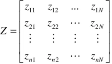
3.1. NONLINEAR REGRESSON MODEL
An arrangement is conformed having a line for each
one of the
n
geometric variables measured for eachsection, and a column for each one of the
N sections. This arrangement is called matrix of
observation X (regresor space).
=
nN n n N Nz
z
z
z
z
z
z
z
z
Z
2 1 2 22 21 1 12 11...
Traditionally, the clustering terminology defines the columns of the matrix of observation X as characteristics or attributes, while the lines are called patterns or objects.
4. FUZZY CLUSTERING LOGIC
It is defined as cluster, the sub-set of data that are
more similar between them than with other data from another sub-set.
There are different types of data association or clustering, one of the most popular is the “Hard clustering” which refers to grouping the data in
specific clusters mutually exclusive (see Figure 3), meaning that a data belongs only to one cluster and not to several clusters at the same time. In figure 3 the data z5 could belong to both clusters
c
1andc
2, this data is not had into account when using the Hard cluster.Figure 3. Data set
(Delf center for System, TU Delft, BABUSKA. R)
It is reasonable to think that in the frontier of two clusters
c
1 andc
2 there are some points that have a degree of belonging in both cluster. The algorithm c-means (Bezdek in Jang, 1997) allows that each pointbelongs to a cluster with certain degree of belonging, so each point belongs to several clusters. This makes
the fuzzy clustering, in some real situations, to be more natural than the Hard clustering.
4.1. Partition Fuzzy
The objective of the clustering is to divide the data set Z =
{
z1,z2,,zN}
inc
clusters (2≤c≤N ),that partitionU =[uik], where uik is the degree of
belonging of the i point to the cluster k. U represents a fuzzy partition if the points fulfil the following conditions:
[ ]
0,1 ∈ik
u 1≤i≤c, 1≤k ≤N, (4.1.1)
∑
= = c i ik u 11 1≤k≤ N (4.1.2)
∑
= < < N k ik N u 10 1≤i≤c, (4.1.3)
Definig the fuzzy partition space as:
[ ] ∀ < < ∀ = ∀ ∈ ℜ ∈ =
∑
∑
= = c i N k ik ik ik cxNfc U u i k u k u N i
M 1 1 , 0 ; , 1 ; , , 1 , 0
4.2. Algorithm Fuzzy C-Means
There are different algorithms for fuzzy clustering, the most used is the “C-Mean” algorithm. This algorithm makes the data partition minimizing the objective function [6]:
(
)
∑∑
= = = c i N k ik m ik d u V U Z J 1 1 2 ,; (4.2.1)
Where:
{
z z zN}
Z = 1, 2,, (4.2.2)
Is the data set to classify.
[ ]
uik MfcU = ∈ (4.2.3) Is the partition matrix Z.
[
v1,v2 ,vc]
,V = n
i
v ∈ℜ (4.2.4) Is the centre vector (clusters) to find.
2 2
i k
ik z v
d = − (4.2.5)
Is the Euclidian norm, distance from the data to the center of a cluster.
[
1
,
∞
)
∈
m
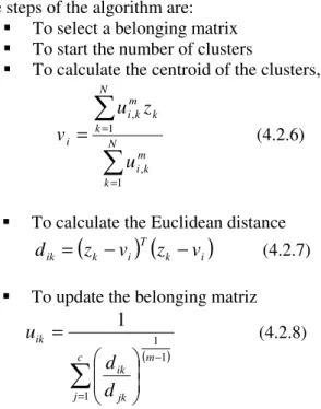
The steps of the algorithm are:
To select a belonging matrix
To start the number of clusters
To calculate the centroid of the clusters,
∑
∑
= = = N k m k i N k k m k i i u z u v 1 , 1 , (4.2.6)To calculate the Euclidean distance
(
) (
k i)
T i k
ik
z
v
z
v
d
=
−
−
(4.2.7)To update the belonging matriz
( )
∑
= −
=
c j m jk ik ikd
d
u
1 1 11
(4.2.8)The equation (4.2.6) gives a value
v
1 that is the weighted average of the data belonging to a cluster, where the weights are the belonging functions.This algorithm presents the following disadvantages:
The final results depend on the final
partition.
The number of cluster is defined at the
beginning of the algorithm
The Euclidean distance method allows
detecting only spherical clusters.
This very last disadvantage is a drawback, because the most ideal shape of data grouping is given by an elipse, so the most appropriated algorithm is the one called “Gustafson-kessel”, because this one looks for hyper ellipsoids clusters, which detect very well the quasi-lineal behaviour of the data.
Figure 4. Clusters of different shape
(Delft centre for System, TU Delft, BABUSKA R)
4.3. Gustafson-kessel (GK) Algorithm
This algorithm is found among the adaptative distance algorithms. This one extends the fuzzy c-means by choosing a different normBi for each
cluster instead of keeping it constant.
(
)
i(
k i)
T i k
ikB
z
v
B
z
v
d
2=
−
−
(4.3.1)Where Bi are the possible optimisation matrixes of
the objective function, and correspond to the covariance of each cluster.
Then, the objective function is defined as follows:
(
)
∑∑
= = = c i kk uikdikBi V U Z J 1 1 2 ,
; (4.3.2)
In order to obtain a viable solution, Bi must be limited somehow. In this case, we will keep its volume constant by fixing the determinant of Bi.
( )
[
]
12 1
det −
= i i i
i F F
B
ρ
(4.3.3)
Where Fi is the covariance matrix for each cluster.
The GK algorithm fits with the purpose of identification because it has the following characteristics:
The cluster dimension comes limited by the
measure of the distance and by the definition of the clusters prototype as a point.
In comparison with other algorithms, GK is
relatively insensitive to the initialization of the partition matrix.
Once we have the groups of data, the next step is to derivate the interference rules which identify a fuzzy model. To achieve that, there are different types like:
Mandami: Fuzzy rules with fuzzy antecedents and fuzzy consequents.
Because the TS fuzzy model is an effective tool for the approximation of nonlinear systems based in the information of inputs and outputs through interpolation of the local linear models, which for this case are determined by the cluster, we use this TS model in the solution of the identification of the model we are looking for.
The solution consists of projecting the belonging of the obtained cluster in the desired space (Figure 5), thus obtaining belonging functions from the cluster.
Figure 5. Extraction of rules by fuzzy clustering
(Delft centre for System, TU Delft, BABUSKA R)
4.4. Takagi-Sugeno Model
In the Takagi-Sugeno model, the consequent rules are function of the inputs:
:
i
R If
x
isAi Then yi = fi(x),i=1,2,....K (4.4.1)Where x∈ℜ is the input variable (antecedent), Ai
is a multidimensional fuzzy set (cluster), yi is the output variable (consequent), Riis the ith rule and K is the number of rules of the rules set.
The consequent function can be linearly expressed as:
i i T
i a x b
y = + (4.4.2)
(4.4.2) in (4.4.1):
:
i
R If
x
isAi Then i iT
i a x b
y = + (4.4.3)
Given the outputs of the individual consequentsyi,
the global output and the Takagi-Sugeno model
(defuzzyfication) is calculated by:
( )
( )
∑
∑
= =
=
Ki i K
i i i
x
y
x
y
1 1
β
β
(4.4.4)
Where
β
i is the commitment degree of theantecedent of the ith rule, calculated as the belonging degree of x in the interior of the Ai
cluster:
( )
x i( )
xi
µ
β
= (4.4.5)Normalising,
( )
( )
∑
= r
j j i i
x w
x w x
h( ) (4.4.6)
So the TS model could be interpreted as a quasi-linear model with dependence on the input x parameter.
( )
(
)
∑
=⋅
⋅
+
=
ri i
T i
i
x
a
x
b
h
y
1 (4.4.7)
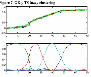
Figures 6 and 7 show an example of a functiony = f(x), represented by four TS rules. The antecedent of each rule defines a valid zone (fuzzy) for the correspondent linear model of the
consequent. The global output function yis
calculated through the weighting of the local linear models.
Figure 6. Takagi-Sujeno fuzzy clustering
Figure 7. GK y TS fuzzy clustering
5. NUMERICAL RESULT
During this work, the toolbox developed by the professor Robert Babuska [13] from the Delft Centre for System and Control was used. This tool was developed to be worked on MATLAB.
Once the information is collected from the matrix of observationsX , is taken to a pre-processing that consists in centering the matrix.
Figure 8. Normalization of a matrix
Where x is the measure of each variable
S is the standard deviation.
The quality of the model is evaluated by calculating the average error (equation (2.3)), its equivalent in the used toolbox, corresponds to the percentile variance accounted (VAF)[13], between the real and the estimated data.
This coefficient is obtained between two signals:
(
)
( )
−− ⋅ =
1 var
2 1 var 1 % 100
y y y
VAF (5.1)
Where the value of VAF will be 100% if both signals are equal. If the values are quite different, the value of VAF will tend to zero.
For each vehicle, the following procedure was followed:
The matrix is normalised.
The matrix is divided into two sections, one for
the identification of the model and the other to carry out the verification of the obtained model.
The real acceleration with the obtained model by
multiple linear regression was plotted [14],[15]. This was also used to determine the ride quality model [16], because of that it will be a reference to validate our results and the obtained result by the fuzzy clustering method.
The VAF coefficient is calculated to determine the accuracy of the model compared with the real data.
The best results were obtained using the toolbox with the following parameters:
FM.c = 12; % number of clusters
FM.m = 2.8; % fuzziness parameter
FM.tol = 0.1; % termination criterion
FM.ante = 2; % 2 - projected MFS FM.cons = 2; % 2 - weighted LS
Where FM is the defined structure by Babuska in MATLAB for the parameters of the toolbox.
In table 3, we present the obtained results with the fuzzy nonlinear regression model and the obtained results with the multiple regression model [16].
Table 3. Results
Item Unidad
Regresión Lineal(%VAF)
Fuzzy Clustering(%VAF)
1 05 76.16 100
2 09 97.52 100
3 10 80.01 95.53
4 12 86.89 100
5 13 87.03 99.17
6 15 78.69 100
7 17 87.19 100
8 19 92.66 100
9 22 86.81 100
10 24 94.7 100
11 34 84.93 100
12 35 70.86 99.07
13 38 77.83 100
15 41 92.5 92.6
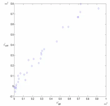
Figure 9 shows the measured data of the acceleration and the model output data obtained by fuzzy clustering for the vehicle 05. It is noticeable that in the table of results there is a VAF of 100%, that corresponds with the line at 45º of the figure and besides produced faithfully the acceleration as it is shown in figure 10.
Figure 9. Plot Yqst vs. Output fuzzy model Vehicle 05.
Figure 10. Real acceleration curve vs. Model curve Vehicle 05.
In table 3 it is observed that the worst VAF coefficient corresponds to the vehicle 40, with a VAF of 92.28. If we plot the data (see figure 12) it can be clearly observed which model did not estimated well a data, leaving this out of the
comparative graphic of 45º (Figure 11). This could be because of tunning problems of the model, either in the sensors installation, different geometric conditions of the rail or the equipment capacity, etc.
Figure 11. Plot Yqst vs. Fuzzy model output. Vehicle 40
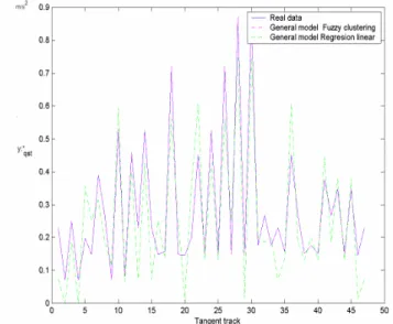
To obtain a general model, all the samples of the 15 vehicles in a matrix were taken, and then a pre-processing consisting of interchanging the files randomly was made. After that, the same process made to the vehicles individually was made and the results were a VAF of 97.35. It can be graphically observed in figures 13 and 14.
Figure 13. Plot Yqst vs. Fuzzy general model output.
Figure 14. Real acceleration curve vs. General model Curve
6. CONCLUSIONS
In this article, the main Fuzzy clustering aspects for the model identification were revised.
Although the obtained results with the linear multiple regression are satisfactory, comparing the obtained results, we find that the quality of the fuzzy model is better in 14 out of 15 analysed vehicles, and only one vehicle of the model of linear multiple regression is better than with the fuzzy model.
We showed that Fuzzy clustering is a good tool to approximate nonlinear functions, specially the Takagi-Sugeno model.
This regression model can be integrated into the process for decision support in maintenance rail-vehicle interface. To reduce the cost associated in the maintenance work, human resources and increase the reliability of system.
Due to the reasons explained before, when it comes to identify a nonlinear model, we recommend the fuzzy model to be used in future implementations among the SPD.
7. ACKNOWLEDGEMENTS
We would finally like to express deep gratitude to EAFIT University, COLCIENCIAS and the Medellín Metro Company for making possible the execution of this document.
REFERENCES
[1] DE VEAUX R, SCHUMI J, SCHWEINSBERG J, UNGAR L Predection intervals for Neural Networks via nonlinear regression
Technometrics, vol.40, Issue 4, 1998 pag 273-282 ISSN:0040-1706 USA
[2] HORNIK K, STINCHCOMBE M, WHITE H Multilayer feedforward networks are universal approximators
Neural Networks Vol. 2, Issue 5,1985 pag 359-366 ISSN:1045-9227
[3] MHASKAR H.N. Neural networks for optimal approximation of smooth and analytic functions Neural computation, vol 8, 1996 pag 164-177 ISSN:0899-7667
[4] CHEN S, BILLINGS S.A. Representation of non-linear system: the NARMAX model
International journal control 49 pag 1012-1032
[5] SPECHT D.F A general regression neural network IEEE transactions on Neural networks, Vol.2 Issue 6 1991
ISSN: 1045-9227
fuzzy models. Published Springer- Berlin- 2001 ISBN 3–540–67369–5
[7] INTERNATIONAL UNION OF RAILWAYS.
UIC CODE 518. Testing and approval of railway vehicles from the point of view of their dynamic behaviour – safety – track fatigue – ride quality. 2nd edition, April 2003. 72 p.
[8] BABUSKA R., Fuzzy modeling for control.
Kluwer Academic publishers. 1998 ISBN:
978-0-7923-8154-9
[9] KUMAR M, STOLL R, STOLL N., A min-max approach to fuzzy clustering, estimation, and identification. IEEE transactions on fuzzy system, Vol 14, No 2, 2006 pp 248-262 ISSN: 1063-6706
[10] HWANG C, CHUNG-HOON RHEE F, Uncertain fuzzy clustering: Intervak type-2 fuzzy approach to C-means. IEEE transactions on fuzzy system, Vol 15, No 1, 2007 pp 107 120. ISSN: 1063-6706
[11] HONDA K, ICHIHASHI H, Regularized linear fuzzy clustering and probabilistic PCA mixture models, IEEE transactions on fuzzy system, Vol 13, No 4, 2005 pp 508-516 ISSN:1063-6706
[12] TAKAGI, T. SUGENO, M. Fuzzy
Identification of systems and its applications to modeling and control. IEEE Transactions on systems, man, and Cybernetics. Vol. SMC-15. 1985. pp.116-132.
[13] BABUSKA R, Fuzzy modeling and identification toolbox
[14] WALPOLE, Ronald E. y MYERS, Raymond H. Probabilidad y estadística. Ed. 4. México : Mc Graw Hill, 1992, 797p. ISBN 968-422-992-5.
[15] KREYSZIG, Edwin. Introducción a la estadística matemática: principios y métodos. México : Editorial Limusa S.A. 1978, 505p.
[16] ZOLTOWSKI B, CASTAÑEDA L,
BETANCOURT G, Monitoreo Multidimensional de la Interfase Vía-Vehículo de un Sistema Ferroviario Congreso Internacional de Mantenimiento – ACIEM – Marzo 2007. Bogotá Colombia
[17] M. ISHIDA, M. AKAMA, K. KASHIWAYA,
A. KAPOOR « The current status of theory and practice on rail integrity in Japanese railways— rolling contact fatigue and corrugations ».
Fatigue & Fracture of Engineering Materials and Structures, Vol. 26. No 10. 2003. pp.909-919.
[18] ZOETEMAN, A. ESVELD, C. « State of the art in railway maintenance management: planning systems and their application in Europe ».
Systems, Man and Cybernetics, 2004 IEEE International Conference on. Vol. 5. 2004. pp.4165-4170.
[19] OTTOMANELLI M, DELL'ORCO M, SASSANELLI D. « A Decision Support System Based on Neuro-Fuzzy System for Railroad Maintenance Planning ».
http://dblp.uni-trier.de
[20] DEBIOLLES A, OUKHELLOU, L. AKNIN, P. « Combined use of partial least squares regression and neural network for diagnosis tasks ».
Pattern Recognition, 2004. ICPR 2004. Proceedings of the 17th International Conference on. Vol. 4. 2004. pp.573-576.
[21] DEBIOLLES A, OUKHELLOU, L. AKNIN, P. « Linear and nonlinear regressions using PLS feature selection and NN on defect diagnosis application».
Int. Conf. On Machine Intelligence ICMI 2005.
[22] CASTAÑEDA L, ZOLTOWSKI B « Diagnostic System for the metro train ».
International Conference on Maintenance
Engineering (ICME), Cheng Du, China. October 15-18, 2006.
[23] CASTAÑEDA L, ŻÓŁTOWSKI B Metoda
środowiskowych badań pojazdu szybowego.
Inżyniera i Aparatura Chemiczna. SIMPress,
Gliwice, Poland. 3 specjalne maj 2006 Pag. 100-104. ISSN 0368 - 0827
[24] CASTAÑEDA L, ŻÓŁTOWSKI B

![Table 1 presents the different estimators considered by the standard. It was necessary to acquire acceleration and forces signals in different parts of the train to calculate the estimators [5]](https://thumb-us.123doks.com/thumbv2/123dok_es/6899122.843412/3.918.480.845.77.396/different-estimators-considered-necessary-acceleration-different-calculate-estimators.webp)