Takagi-Sugeno fuzzy incremental state model for optimal control of a ball and beam nonlinear model

Takagi-Sugeno Fuzzy Incremental State

Model for Optimal Control of a Ball

and Beam Nonlinear Model

Basil M o h a m m e d Al-Hadithi Jose Miguel Adanez and Agustin Jimenez

A b s t r a c t . The optimal control of a ball and beam by an approach based on Takagi-Sugeno incremental state model is proposed. The advantages of incremental state model in comparison with the non incremental one are that the control action cancels steady state errors, the affine terms disappear and incremental state solves the problem of computing the tar-get state, choosing zero as an objective. A generalized version of Takagi-Sugeno identification method is applied. For an optimal control, Linear Quadratic Regulator and optimal state observer are used in each fuzzy rule. Simulation results over the ball and beam nonlinear model show a stable closed loop in the full range, zero steady state error and good transient response.

1 I n t r o d u c t i o n

T h e ball and b e a m system [1] is a classical mechanical system with two degrees of freedom. T h e b e a m rotates, driven by a torque at t h e center of rotation. T h e ball rolls freely in contact with t h e b e a m . In spite of its mechanical simplicity, t h e ball and b e a m system is nonlinear and unstable which presents significant challenges from t h e control point of view.

T h e ball and b e a m is a common didactic plant in m a n y control laboratories [2], as it is nonlinear, unstable, which means t h a t it is difficult t o control, and can be a b e n c h m a r k for testing several advanced control techniques [3].

In [5], an approach developed by the authors is presented to improve the esti-mation of T-S models. The problem is that the original T-S identification method cannot be applied when the triangular membership functions are overlapped by pairs. This restricts the use of this type of membership functions which have been widely used in the controllers design and are popular in industrial applica-tions. The approach, to search for an exact optimal solution, uses the minimum norm method although it increases complexity and computational cost. Another approach was developed in [6], which can be considered as a generalized version of T-S method. This simple method with not much computational cost is based on weighting of parameters. In [7], this T-S identification method was extended to the multivariable case. These methods are characterized by the high accuracy obtained for modelling nonlinear systems in comparison with the original T-S method [4].

Incremental state model is presented in [8] to model multivariable nonlin-ear delayed systems expressed by a generalized version of T-S fuzzy model. The advantages of incremental state model compared with non incremental one has been defined. First, it solves the problem of computing the target state, choosing zero incremental state as an objective. Second, the control action in an incre-mental form is equivalent to introduce an integral action. Third, increincre-mental state model makes the affine terms disappear. A comparative analysis has been developed in [9] between incremental state model and traditional one, the con-trol based on these state models have been developed by a linearized model and applied over a nonlinear model of a wind turbine.

The rest of the work is organized as follows. Section 2 describes ball and beam nonlinear model. The fuzzy T-S model and the fuzzy identification method are described in Sect. 3. In Sect. 4, incremental state model is presented. Optimal state controller and optimal state observer designs are described in Sect. 5. In Sect. 6, the proposed fuzzy optimal controller based on incremental state model is applied to the ball and beam nonlinear model.

2 Ball a n d B e a m Nonlinear Model

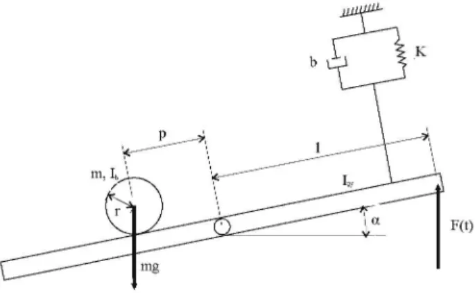
In this work, the AMIRA BW500 (Fig. 1) [1] is used as ball and beam model. The ball position p, the objective system output, would be measured by a camera, therefore the discrete sample time is supposed to be large. The beam angle a would be measured by an incremental encoder, thus it is considered as a measurable internal variable. The system input F is a force produced by a DC motor, which causes the beam to rotate around its center.

The nonlinear differential equations of the ball and beam model [1] are:

m -\—2 ) P + (m r + lb) ~& ~ mpa = mgsm(a) (1)

(mp2 +Ib + Iw) a + (2mpp + bl2) a + Kl2a+

1 .. (2)

Fig. 1. Ball and beam system.

where p is the ball position, a is the beam angle and F is the drive mechanics force. Table 1 summarizes the model parameters and its values.

Table 1. Ball and beam parameters

Parameter

m

9 r h Iw b

K I

Meaning Mass of the ball Gravity

Roll radius of the ball Inertia moment of the ball Inertia moment of the beam

Friction coefficient of the drive mechanics Stiffness of the drive mechanics

Radius of force application

Value 0.025 Kg 9.81 m / s2

0.0f67m

3.516 - f O ^ K g m2

0.09 Kgm2

f.ONs/m 0.001 N / m 0.49 m

Since we consider a as a measurable internal variable, the system is modeled as single-input-single-output (SISO), and the relation between output p and input F is described by two second order differential equations, so the global system is fourth order.

3 Fuzzy Takagi-Sugeno Model and System Identification

3.1 Fuzzy T-S Model

Nonlinear systems can be modelled by T-S model, supposing known a set of measurable nonlinear variables [zi(k), Z2(k),..., zm(k)] of the system. By

system can be defined as follows:

S{ii-im). I f Zi(kj i g Mh a n d _ a n d Zm(kj i g Mi „ t h e n.

y(fc) = at-im) + at-im)y{k -!) + ••• + a^-A^y{k - n) (3)

+ 6(1il'"im)w(A; - 1) + • • • + b^-im)u(k - n)

In each rule, we can transform the difference equation (3) to state model with affine term as follows:

S{ii-im). I f Zi(kj i g Mh a n d _ a n d Zm(kj i g Mi^ t h e n. x(jfe) G 9 T

x(> + 1) = (h-irr,

a0

(ii-im a0

(h-irr,

a0

' UJ-\

• a2

Ul-.-im.)

+

•f f l( i i . . . im

at

—

a^...im

> i

-V

>o-• 0

• 0

. 1 • 0

x(k) +

•6( i i . . . im) "

i{i\—im)

°2

Ai\—im)

l(k) = a!i1-im)+[lO---0]x(k)

u{k)

(4)

In matrix form:

s(h-im). I f Zl(kj i s Mh a n d _ a n d Zm(kj i s Mhr, t h e n.

x(jfe + 1) = of.'1-'"' + A ^ - ^ x ^ ) + B^-A^u{k) (5)

y ( » = a(,i l-i r o )+Cx(A;)

3.2 Estimation of T-S Model Parameters

The identification method of T-S fuzzy models [4] is based on the estimation of the fuzzy system parameters minimizing a quadratic performance index. The traditional T-S identification method [4] fails if the triangular membership func-tions are overlapped by pairs, since the T-S matrix is not of full rank and then it is not invertible [5]. Thus, in [6] a generalized T-S identification was proposed, using a parameters weighting method.

The fuzzy estimation of the output becomes:

= E-"E^

-

(^

...o(*))

£ l = l I™ = 1 (6)

+ a^-im)y(k - n) + 6(1il"'im)w(A; - ! ) + ••• + b^-im)u(k - n)

where

/ ?( < 1-i m ) (*(i!...im)W) =

• ferritin \^m)

J2i11=i---J2iZ=i(Pih(zi) .(!,„ ,{zm))

with /Zjj. (ZJ) being the membership function corresponding to the fuzzy set M*3. It is supposed to have a set of input/output system samples and a first affine linear parameters estimation p° = [a§ a° . . . a° 6° • • • ^n] y which could be obtained by a classical input/output identification of the data, for example with least squares method. This first approximation can be utilized as reference parameters for all the subsystems. Then, the fuzzy model parameters can be obtained minimizing:

r-m ri

2

fc=l

(8)

\Y-XP\\z+12\\Po-P\\ Y X P

where Y are the output data, X are the input/output fuzzy data, PQ are the linear estimated parameters repeated as many times as the number of fuzzy rules (Po = \po,Po, • • • ,Po]), a n (i P are the fuzzy T-S model parameters. The 7 factor represents the degree of confidence of the linear estimated parameters, and it must be adjusted. It should be noted that the matrix Xa is of full rank, even if

the membership functions are triangular overlapped by pairs, which solves the problem where the traditional T-S identification method fails. Thus, the vector P can be computed as:

P — \XaXa) XaYa (9)

4 Incremental State Model

The control method based on traditional state model, can produce steady state errors in presence of disturbances or modelling errors. This problem can be solved by incremental state model [8,9].

Applying the discrete state model described in (5), at the previous sample ( * - l ) :

x(k) = ax + Ax(k - 1) + Bu(k - 1)

y(k - 1) = ay + Cx(k - 1)

Subtracting (10) from (5):

x(k + 1) - x(k) = A (x(k) - x(k -1)) + B (u(k) - u(k - 1))

y{k)-y{k-l) = C{x{k) -x(k-l)) (11)

where the affine terms are cancelled. Defining the incremental state Ax and the incremental input Au as follows:

Ax{k) = x{k) — x{k — 1) Au{k) = u{k) — u{k •

Substituting (12) into (11), it is obtained:

Ax(k + 1) = AAx(k) + BAu(k) y(k) =y(k-l) + CAx(k)

1) (12)

A new state is introduced to complete the formulation, verifying that:

y(k + 1) = y(k) + CAx(k + 1) = y(k) + C (AAx(k) + BAu(k)) (14)

A new expanded incremental state vector xa G 9\(1+n'> is defined, obtaining the

new state model as follows:

(15) y(k+l) '

^x(k+ 1)

y(k =

) =

"1 CA 0 A

1 0 ] " y A

' y(k) ' Ax{k)

(k) 1

x{k)

+

X

CB B

a(k)--Au{k)

' y(k) ' Ax(k)

In matrix notation, the expanded state model becomes:

xa{k + 1) = Aaxa{k) + BaAu{k)

y(k) = Caxa(k)

(16)

Using the method described in Eq. (15) in each fuzzy rule defined by T-S state model (5), an incremental T-S state model can be obtained as follows:

S(ii-im). I f ^ ( f c ) i s Mn a n d . . . a n d 2m(fc) i s Mi™. t h e n :

xa(k + 1) = A^-^Xaik) + B^-^Auik)

y(k) = Caxa(k)

(17)

5 Fuzzy Controller and Observer Design Based

on I n c r e m e n t a l S t a t e Model

5.1 Fuzzy Controller for Zero Steady-State Error

Incremental state feedback control can be designed by any method. In order to calculate the coefficients of the state feedback controller, discrete LQR method is chosen, which allows optimal control weighting the dynamic response and the control action.

The goal is to minimize the cost index J:

J =

fc=0

(xr - xa(k)Y' Q (xr - xa(k)) + Au{kYRAu{k) (18)

If the control objective is to approach a steady state output yr, this is

equiv-alent to achieve the reference expanded state in incremental model [8,9]:

Vr

Axr

Vr 0

Then the control action is described as:

S{ii-im). I f Zl(kj i s Mii a n d _ a n d Zm(kj i s Mi™ t h e n.

Au{k) = K {xar - xa{k)) = K{il-im) Vr ~ v(k)

-Ax{k)

u(k) =u(k - l) + Au(k)

(19)

(20)

It should be noted that the reference expanded state comes naturally without any calculations. Moreover, control action (20) is calculated in incremental form

(19), which is equivalent to apply an integral control action. If the feedback system is stable and the steady state is approached, the controlled system has zero steady state error [8,9].

5.2 Fuzzy Observer for Incremental State Model

In the controller algorithm it is supposed that the output y(k) is measurable, but the incremental state Ax(k) is not directly accessible, then a state observer is required. The state observer is a parallel dynamic system with a correction term that approximates the estimated state to the real one. The fuzzy incremental state observer [8,9], is formulated as follows:

S{ii-im). I f Z i ^ i g Mi i a n d _ a n d Z m ^ i g Mi^ t h e n.

Axe(k + 1) = A{il-im)Axe(k) + B{h-im) Au(k)+

Thus, the expanded estimated state is obtained as follows:

(21)

•^ae\"'j v(k)

Axe(k)

(22)

Matrix H^-A^ e m{nxl) coefficients are obtained by optimal state observer

design [8,9] in each fuzzy rule.

The optimal observer solves the problem of calculating a matrix H which minimizes the cost index J„:

J0(H) = aT (A- HC) (A - HC)T a

It is verified in [8] that for any value of a, it fulfills:

H = ACT(CCT)-1

\/aem

In t h e proposed s t a t e representation C m a t r i x is defined in observable canonical form, therefore it holds t h a t CCT = I, so t h a t :

H = ACT (25)

T h e separation principle holds between optimal observer and control design.

6 Results

T h e ball and b e a m model is defined in continuous time, b u t t h e controller has been developed in discrete time, therefore, a sampler and zero order hold-ing device have been added t o t h e model, with t h e proposed samplhold-ing time

T = 0.05 s. All system variables are supposed t o be ideally measured.

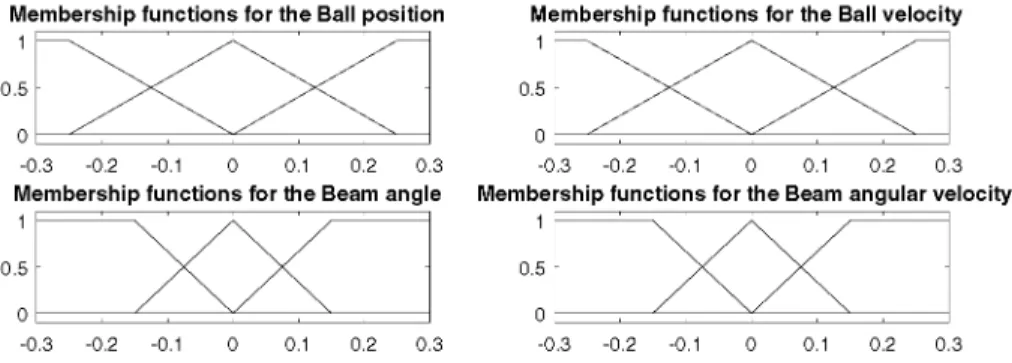
For a generalized T-S identification of t h e system, t h e following weighting factor 7 = 1 0- 1 1 and t h e following membership functions defined in Fig. 2 has

been chosen, obtaining an identification error of 1.6169 • 1 0- 1 1.

Membership functions for the Ball position

1

Membership functions for the Ball velocity

-0.3 -0.2 -0.1 0 0.1 0.2 0.3 -0.3 -0.2 -0.1 0 0.1 0.2 0.3

Membership functions for the Beam angle Membership functions for the Beam angular velocity

1

-0.3 -0.2 -0.1 0 0.1 0.2 0.3 -0.3 -0.2 -0.1 0 0.1 0.2 0.3

Fig. 2. Membership functions of the fuzzy sets.

W i t h t h e generalized T-S identification m e t h o d and Eq. (15), a fuzzy T-S incremental s t a t e model has been obtained:

?(i,1,1,1).

y(k + l) Ax(k+1)

If p(k) is Mi and p(k) is M2 and a(k) is M3 and a(k) is M4 then:

1 3.9181 1 0 0' 0 3.9181 1 0 0 0 -5.7542 0 1 0 0 3.7543 0 0 1 0 - 0 . 9 1 8 1 0 0 0

Axik) + 10"

-0.0502 -0.0502 0.1562 0.1262 -0.0571

Au(k)

y(k) = [ 1 0 0 0 0] Axik)

definite weighting matrices Q = I and R = 1. T h e observer m a t r i x is defined by t h e optimal s t a t e observer m e t h o d [8,9], using Eq. (25). Obtaining:

5(1,1,1,1). ifp^ i s Mi a n d p ^ i s Mi a n d a(j^ i s Mi a n d d^) i s Mi t h e n :

^(1,1,1,1) = 1 0 3 [0.0008 4.0174 3.2390 2.5627 1.9811]

# ( i , i , i , i ) = [3.9181 - 5 . 7 5 4 2 3.7543 - 0 . 9 1 8 1 ] *

W i t h this fuzzy controller and observer design method, t h e global stability cannot be theoretically proved, so it has t o be analyzed a posteriori with t h e simulation results.

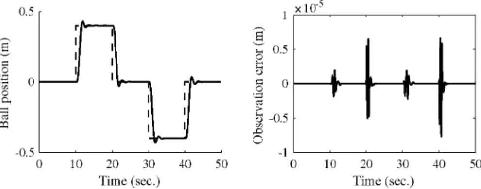
Figure 3, shows t h e ball position and t h e observation error of t h e ball position, when t h e controlled system is subjected t o changes in t h e ball position reference. Moreover, Fig. 4 shows t h e b e a m angle and t h e input force.

xlO

10 20 30 Time (sec.)

50 20 30 40

Time (sec.)

50

Fig. 3. Ball and beam variables: (left) Ball position, (right) Observation error of ball

position.

u

s

-a

3 D-C

0.5

•0.5

m T

10 20 30 40 Time (sec.)

50 10 20 30 40

Time (sec.)

50

In Fig. 3 (left) it can be seen that the system present stable and good tran-sient response and zero steady state error. In Fig. 3 (right) it is shown that the observation error is of small range and tends to zero. In Fig. 4 it can be seen that, the system variables present smooth and stable transient responses. Thus, the controlled ball and beam model has a stable response in the full range of the system, presents a good transient response and zero steady state error.

7 Conclusion

In this work, we have shown the obtained results of T-S incremental state model and optimal state controller and observer, applied in a ball and beam nonlinear model. The advantages of incremental state model over traditional one comes in a natural way and they are that the affine terms disappear, the problem of computing the target state is solved and the control action cancels steady state errors. The optimal controller and observer has been designed in each fuzzy rule, so a suboptimal solution have been found, but easy of calculate and compute. The results show that the ball and beam controlled nonlinear model has a stable behavior, good transient response and zero steady state error on the full range of the ball and beam system.

Acknowledgements. This work is funded by the Spanish Ministry of Economy and