Study of the effects of moving targets in SAR images for their detection.

(1)

UNIVERSIDAD POLITÉCNICA DE MADRID

ESCUELA TÉCNICA SUPERIOR DE INGENIEROS DE TELECOMUNICACIÓN

TRABAJO FIN DE GRADO

(2)

(3)

TÍTULO:

STUDY OF THE EFFECTS OF MOVING TARGETS IN SAR IMAGES FOR THEIR DETECTION

AUTOR:

JULIO ALBERTO GONZÁLEZ MARÍN

TUTOR:

JOSÉ TOMÁS GONZÁLEZ PARTIDA

MIEMBROS DEL TRIBUNAL:

PRESIDENTE: FÉLIX PÉREZ MARTÍNEZ

VOCAL: MATEO BURGOS GARCÍA

SECRETARIO: JOSÉ TOMÁS GONZÁLEZ PARTIDA

SUPLENTE: ALBERTO ASENSIO LÓPEZ

(4)

(5)

UNIVERSIDAD POLITÉCNICA DE MADRID

ESCUELA TÉCNICA SUPERIOR DE INGENIEROS DE TELECOMUNICACIÓN

TRABAJO FIN DE GRADO

(6)

(7)

Abstract

Synthetic Aperture Radar’s (SAR) are systems designed in the early 50’s that are ca-pable of obtaining images of the ground using electromagnetic signals. Thus, its activity is not interrupted by adverse meteorological conditions or during the night, as it occurs in optical systems.

The name of the system comes from the creation of a synthetic aperture, larger than the real one, by moving the platform that carries the radar (typically a plane or a satelli-te). It provides the same resolution as a static radar equipped with a larger antenna. As it moves, the radar keeps emitting pulses every 1/PRF seconds —the PRF is the pulse repetition frequency—, whose echoes are stored and processed to obtain the image of the ground.

To carry out this process, the algorithm needs to make the assumption that the tar-gets in the illuminated scene are not moving. If that is the case, the algorithm is able to extract a focused image from the signal. However, if the targets are moving, they get unfocused and/or shifted from their position in the final image. There are applications in which it is especially useful to have information about moving targets (military, rescue tasks, study of the flows of water, surveillance of maritime routes...). This feature is called Ground Moving Target Indicator (GMTI). That is why the study and the development of techniques capable of detecting these targets and placing them correctly in the scene is convenient.

(8)

Resumen

Los Radares de Apertura Sintética (SAR por sus siglas en inglés) son sistemas dise-ñados a principios de los años 50 que permiten obtener imágenes del suelo usando señales electromagnéticas. Por lo tanto, su actividad no se ve interrumpida por condiciones me-teorológicas adversas o en la noche, tal como si ocurre en los sistemas ópticos.

El nombre del sistema viene de la creación de una apertura sintética, mayor que la real, moviendo la plataforma que lleva al radar (típicamente un avión o un satélite). Proporciona la misma resolución que un radar estático equipado con una antena mayor. Conforme se va moviendo, el radar va emitiendo pulsos cada 1/PRF segundos —la PRF es la frecuencia de repetición de pulsos—, cuyos ecos son almacenados y procesados para obtener la imagen del terreno.

Para llevar a cabo este proceso, el algoritmo necesita hacer la asunción de que los blancos presentes en la escena iluminada no se están moviendo. Si ese es el caso, el algo-ritmo es capaz de extraer una imagen enfocada de la señal. Sin embargo, si los blancos se están moviendo, son desenfocados y/o desplazados de su posición en la imagen final. Hay ciertas aplicaciones en las que es especialmente útil tener información acerca de los blan-cos móviles (militares, tareas de rescate, estudio de los flujos de agua, vigilancia de rutas marítimas...). Esta característica se llamaGMTI —de sus siglas en inglés Ground Moving Target Indicator—. Esta es la razón por la que el estudio y desarrollo de técnicas para ser capaz de detectar estos blancos y colocarlos correctamente en la escena es conveniente.

En este documento han sido detallados varios de los principales algoritmos GMTI usados en sistemas SAR. Se ha creado un simulador para probar las características de cada algoritmo implementado en una situación general con blancos móviles. Finalmente se han realizado pruebas de Monte Carlo, permitiéndonos extraer conclusiones y estadísticas de cada algoritmo.

(9)

Keywords

SAR, GMTI, DPCA, ATI, RDA, CFAR, RCMC, synthetic, aperture, radar, along, track, interferometry, phase, range, Doppler, algorithm, detection, centroid, squint, adap-tive, Monte Carlo, simulation, migration.

(10)

(11)

Index

Abstract _i

Resumen _ii

Keywords _iii

1. SAR PRINCIPLES 1

1.1. Geometry . . . 2

1.2. Beam pattern . . . 3

1.3. Signal . . . 3

1.4. Pulse compression . . . 6

1.5. Window function . . . 6

1.6. Downsampling . . . 6

1.7. Doppler centroid . . . 7

1.8. Signal domains . . . 7

1.9. Algorithms . . . 8

2. RANGE DOPPLER ALGORITHM 9 2.1. Range compression . . . 9

2.2. Azimuth Fourier transform . . . 11

2.3. Range cell migration correction . . . 13

2.4. Azimuth compression . . . 14

2.5. High squint angles . . . 15

2.6. Final result . . . 16

3. MOVING TARGETS 18 3.1. Range movement . . . 18

3.2. Azimuth movement . . . 21

3.3. Fast moving targets . . . 21

4. DETECTION OF MOVING TARGETS 23 4.1. One channel techniques . . . 23

4.2. Displaced Phase Center Antenna . . . 24

4.3. Along Track Interferometry . . . 25

5. SIMULATOR AND IMPLEMENTATION 27 5.1. Raw data simulation . . . 27

(12)

5.3. Multichannel simulation . . . 31

5.4. Detectors implementation . . . 31

5.4.1. Displaced Phase Center Antenna implementation . . . 32

5.4.2. Along Track Interferometry implementation . . . 33

5.4.3. Adaptive Along Track Interferometry implementation . . . 34

5.4.4. Combination of algorithms . . . 35

6. ALGORITHM COMPARISON 36 6.1. Monte Carlo . . . 36

6.2. Simulations and results . . . 36 6.2.1. Simulation 1 - Scenario 1, Gaussian clutter, low target velocities . 37 6.2.2. Simulation 2 - Scenario 1, Gaussian clutter, low target velocities . 39 6.2.3. Simulation 3 - Scenario 1, clutter with scatterers, low target velocities 40 6.2.4. Simulation 4 - Scenario 2, Gaussian clutter, high target velocities . 42

7. CONCLUSSIONS AND NEXT STEPS 44

REFERENCES A

ACRONYMS B

(13)

List of figures

1.1. Image of Brussels obtained with the Sentinel-1 satellite. Source: ESA . . . 2

1.2. SAR system geometry. Source: [1] . . . 2

1.3. Pulses transmitted and echoes received. Source: [1] . . . 4

1.4. Module of the raw data received from one single target . . . 5

1.5. Phase of the raw data received from one single target . . . 5

2.1. RDA steps. Source: [1] . . . 9

2.2. Positions of each target . . . 10

2.3. Raw data matrix . . . 10

2.4. Range compressed signal in the time domain . . . 11

2.5. Range compressed signal in the range-Doppler domain . . . 12

2.6. Range-Doppler matrix after RCMC . . . 13

2.7. Final SAR image . . . 14

2.8. Final SAR image taken with a system with squint angle . . . 16

2.9. Zoom of the samples of a single point target . . . 17

2.10. Profile in one direction of a single point target . . . 17

3.1. Raw data matrix of the six moving targets . . . 19

3.2. Range-Doppler domain matrix of the six moving targets . . . 19

3.3. Final SAR image of the six targets without filtering . . . 20

3.4. Range-Doppler domain matrix of the six moving targets after filtering . . 20

3.5. Final SAR image of the six targets after filtering . . . 21

3.6. Final SAR image of a moving target with azimuth speed . . . 21

3.7. Final SAR image of three moving targets with different speeds . . . 22

4.1. DPCA scheme. Source: [5] . . . 24

4.2. Final SAR image of one single moving target masked by clutter . . . 24

4.3. Result of subtracting the images of both channels . . . 25

4.4. ATI scheme. Source: [5] . . . 26

5.1. Raw data signal with SNR=20 dB . . . 29

5.2. Final SAR image obtained with the RDA from a raw data signal with SNR=20 dB . . . 29

5.3. CA-CFAR scheme. Source: [7] . . . 33

5.4. ATI detections . . . 34

6.1. Simulation 1 graphic results . . . 38

(14)

(15)

List of tables

5.1. DPCA coefficients . . . 32

6.1. Simulation 1 parameters . . . 38

6.2. Simulation 1 table of results . . . 38

6.3. Parameters used in simulations 2 and 4 . . . 39

6.5. Simulation 3 parameters . . . 41

(16)

(17)

Chapter

1

SAR PRINCIPLES

Synthetic Aperture Radars (SAR) [1] are systems designed to obtain two-dimensional images of the ground surface. The term SAR refers to the concept of creating a very long antenna by signal analysis. The relative motion between the antenna and the tar-gets creates coherent signal variations that can be used to obtain, with digital signal processing (DSP), greater synthetic apertures, and therefore, narrower beamwidths and greater resolutions with relatively small antennas (in the order of 1-15m).

SAR systems make images of the earth by pointing a radar beam approximately perpendicular to the sensor’s motion vector, transmitting phase-encoded pulses, recor-ding the radar echoes reflected off the earth surface and processing them. It is an active system, which means that carries its own illumination, working equally well in darkness. Also the common frequencies of electromagnetic waves pass through clouds, precipita-tion and even vegetaprecipita-tion with either little or no deterioraprecipita-tion. These are very good advantages that optical systems do not have.

They are a derivation of the original radar systems which used time delay, antenna directivity and Doppler shifts to measure the range, direction and radial velocity of a target. They were created in the 1950’s by Carl A. Wiley —a mathematician who was working on a correlation guidance system for the AtlasICBM (Intercontinental Ballistic Missile) program in Arizona— as a military reconnaissance tool, solving the need for a 24h, all-weather, aerial remote surveillance device [2]. They also respond to the need of higher resolutions but with smaller antennas than the ones used in real aperture systems.

In 1978, NASA (National Aeronautics and Space Administration) launched the “SEASAT” satellite; the first civilian SAR application [3]. Since that moment, a lot of improvements have been achieved, including multistatic operation, polarimetry, in-terferometry... but most importantly in the digital processes

Recently, April 2014, a promising radar satellite has been launched to space byESA (European Space Agency): the Sentinel-1 [4].

(18)

1.1. GEOMETRY

ETSI-TELECOMUNICACIÓN

Figure 1.1: Image of Brussels obtained with the Sentinel-1 satellite. Source: ESA

1.1. Geometry

The geometry of a typical monostaticSARis the following. The antenna is mounted on a moving platform such as an aircraft or spacecraft and repeatedly illuminates a ground scene on his side.

Figure 1.2: SAR system geometry. Source: [1]

The direction in which the platform is moving is called the azimuth direction, and the perpendicular, the range direction. There are two velocities to contemplate: the platform velocity (Vs) and the beam velocity (Vg). We will consider a flat earth model, in which both velocities are equalVs=Vg=Vr.

(19)

1.2. BEAM PATTERN

The most importantSAR parameter is probably the slant range R from the sensor to the target. In the flat earth model, it takes a hyperbolic form:

R(η) =

q

R2₀+ (Vrη)2 _'_R 0+

(Vrη)2

2R0 (1.1)

η is the azimuth time referenced to the time of closest approach. The last approxi-mation can be made only if a low squint angle is being used.

1.2. Beam pattern

MostSARradar antennas have the following approximate azimuth one-way pattern:

pa(θ) =sinc(0,886×θ

βbw

) (1.2)

whereβbw= (0,886×λ)/La is the azimuth beamwidth andθis the angle measured from boresight in the slant range plane. λis defined as λ=c/f0, beingf0 the central frequency of the radar signal and La is the antenna length along the azimuth direction. The received signal strength is given by the square of pa(θ), because of the two-way

propagation of the radar energy.

wa(η) =pa(θ(η))2 (1.3)

The target is illuminated by the beam center at the "beam center crossing time":ηc. The pattern in the range direction is more diverse and depends on the implementation of the specific system, but it is usually weighted to be higher at larger angles to compensate for the 1/R4 law of the radar equation.

1.3. Signal

The most commonly used pulse in SAR is:

spul(τ) =wr(τ)×cos(2πf0τ +πKrτ2) (1.4)

where wr(τ) = rect(τ /Tr) is a rectangular pulse centered at τ = 0 and of duration Tr. Kr is the linear FM rate of the signal. This signal is chosen because it has very important compression characteristics as we will explain later.

The radar transmits coherent pulses evenly spaced —PRI seconds, the inverse of thePRI is thePRF and is the sampling frequency in the azimuth direction—. Cohe-rency means that the start time and phase of each pulse is carefully controlled; this is important in SAR systems to obtain high azimuth resolution.

The signal received from a single point target (scatterer) at a slant range Ra is:

sr(τ) =A×spul(τ−

2Ra

c ) =A×wr(τ−

2Ra

c )×cos(2πf0(τ−

2Ra

c )+πKr(τ−

2Ra c )

(20)

1.3. SIGNAL

where A models the amplitude of the received signal due to the radar equation, c is the speed of light in the media and2Ra/cis the delay. When the radar is not transmit-ting, it can receive echoes reflected from each scatterer, which are added resulting in a non-recognizable waveform. The process is illustrated in figure 1.3

Figure 1.3: Pulses transmitted and echoes received. Source: [1]

The received signal is demodulated by a quadrature demodulation process. The re-sulting signals of this process can be expressed by the following complex representation:

s0(τ, η) =A0×wr(τ −

2R(η)

c )×wa(η−ηc)×e

−j4πf0R(η)/c_×_ejπKr(τ−2R(η)/c)2 (1.6)

The signal is now sampled. Its bandwidth is |Kr| ×Tr and since it is complex, its sampling rate is:Fr =|Kr| ×Tr×α, whereαis the oversampling factor, usually around 1.4.

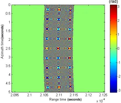
The resulting signal can be considered as two dimensional. Each ground echo is written into one row of SAR signal memory. As the sensor advances more pulses are transmitted and are written into successive rows. A single row can be considered, where echoes from the same transmitted pulse can be found; also a single column can be con-sidered, where echoes from the same slant range from the sensor are found. Arranging the signal in that way seems convenient, as we want to make a two-dimensional image of the Earth surface. This two-dimensional signal is usually called the raw data signal, because it has not been processed yet. An example of a simulated raw data signal from one single target is presented in figures 1.4 and 1.5.

We can observe the module and the phase of 5 seconds of the raw data signal caused by one single target situated at 30 km of the radar track, with zero squint angle. The radar velocity is 250 m/s, the antenna length is 1.5 m and thePRF is 1000 Hz.

It can be observed that while the radar approaches the target, its pulses arrive earlier, and when it moves away, its pulses arrive later; this is called the range cell migration (RCM) because one point target crosses from one range cell to another. Furthermore at the time of closest approach the received energy is higher —this is because this is a zero squint scenario, in which the antenna’s beam center, crosses the target at the time of closest approach—. As we can see, the energy of the target has been spread all over the

(21)

1.3. SIGNAL

two dimensional signal. The main objective of aSAR algorithm is to compress all that energy into one single azimuth and range cell: the one in which the target is located.

Figure 1.4: Module of the raw data received from one single target

(22)

1.4. PULSE COMPRESSION

1.4. Pulse compression

In systems like this one, that require high resolutions, it is needed to carry out a process called pulse compression. Two targets separated less time than the pulse length would not be distinguished, so a shorter pulse is needed or at least it has to be obtai-ned by signal processing. High SNR’s are needed to obtain accuracy; this is done by increasing the pulse length or the peak power. Physical limitations often constrain the peak power, so it is common to use a larger pulse and to compress it later with signal processing.

LinearFM signals can achieve great pulse compressions because their matched filter converts them into a sinc function, which is approximately the shortest possible signal of a given finite bandwidth. A linearFM signal has the following form in the time and frequency domains:

sr(t) =rect( τ Tr)×e

jπKr(t−t0)2 (1.7)

Sr(f) =rect( f

|Kr|Tr)×e

−jπf2_/K

×e−j2πf t0 (1.8)

Applying a matched filter cancels the quadratic phase term of the signal spectrum.

H(f) =rect( f

|Kr|Tr

)×ejπf2/K (1.9)

Sout(f) =rect( f |Kr|Tr

)×e−j2πf t0 (1.10)

The resulting signal in the time domain results in a sinc function, which was our goal. This process of pulse compression will be used in theSAR algorithms.

sout(t) =|Kr|Tr×sinc(|Kr|Tr(t−t0)) (1.11)

1.5. Window function

There is usually a compromise between the resolution of the main lobe and the size of the sidelobes in the signals that we are handling. In the previous expressions we have used a rectangular window. With this window we can achieve very good resolutions, but the sidelobes are usually too large (13 dB below the value of the main lobe). This can cause contamination of bright targets to weaker ones, so usually other windows are used.

The Kaiser window is a very good one because it has a parameter beta with which we can control the size of the sidelobes, but other windows can also be used.

1.6. Downsampling

As a result of the chosenPRF rate (sampling rate in the azimuth direction) and our oversampling factor in the range direction, our signal is oversampled. This decisions are

(23)

1.7. DOPPLER CENTROID

made for designing purposes and affect to the final image. This can lead to situations in which a target is represented by more than one sample in both the range and azimuth directions. If we wanted to detect moving targets, this would affect our capabilities be-cause we would detect a moving target in more than one cell.

A solution to this issue would be the downsampling of our final image. We can calculate the space sampling rate in the azimuth and range direction, and we can also compute the azimuth and range resolution of our image; therefore we can determine the number of samples that represent one target in each direction. Downsampling our image by those factors, we obtain the matrix we wanted.

Finally we have obtained a SAR image in which each target is represented only by one sample, improving our detection capabilities.

1.7. Doppler centroid

One interesting parameter in the SAR signal context is the Doppler centroid. As the radar moves, the signal received from a scatterer suffers a frequency shift in the azimuth direction due to the relative motion between the platform and the scatterer. The Doppler centroid is the azimuth frequency, or Doppler shift, when the point target is the center of the beam (atη=ηc). It is proportional to the rate of change of R(η):

fηc =

2Vrsin(θsq)

λ (1.12)

whereθsq is the squint angle.

We can appreciate that if the squint angle is zero, the Doppler centroid would be zero, but in a more general case it does not have that value. As we are sampling the azimuth at thePRF rate, we can only see the spectrum in the interval [-PRF/2,PRF/2], so in the general case where the Doppler centroid is not zero, we see an aliased version of our centroid, and we have to shift our spectrum to center it at the Doppler centroid. This is an important step in everySAR algorithm because it is necessary to know the exact frequency of the azimuth signal.

1.8. Signal domains

TheSARdata are acquired in the two-dimensional time domain. The data are often transformed into other domains for processing efficiency reasons. The most important domains are the range-Doppler domain and the two-dimensional spectrum.

(24)

1.9. ALGORITHMS

The two-dimensional spectrum is the result of applying a two dimensional DFT to the time domain signal.

1.9. Algorithms

There are many algorithms used to get an image from our original raw data signal. Each step of each algorithm takes advantage of the benefits of each domain, so they are usually changing the signal between different domains. There is a compromise bet-ween efficiency and accuracy. Some algorithms that achieve good accuracy maintaining certain efficiency are the RDA (Range Doppler Algorithm), the CSA (Chirp Scaling Algorithm) and the ωKA(Omega-K) algorithms. TheSPECAN (SPECtral ANalysis) is a very efficient algorithm, used to form images in real time in applications which do not require a lot of precision.

We will now proceed to explain the RDA in the next chapter as it is the one that has been selected to be implemented in our simulator.

(25)

Chapter

2

RANGE DOPPLER ALGORITHM

Figure 2.1: RDA steps. Source: [1] The Range Doppler Algorithm (RDA) [1] is used to

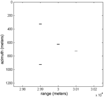
process raw data with the intention of obtaining an ima-ge of the ground being accurate and efficient. The pro-cess is illustrated in figure 2.1. In a low squint scena-rio the azimuth signal and the range signal are almost un-coupled, so we can carry out the processing in each di-rection separately. First of all a range compression is nee-ded. Secondly, an azimuth DFT is done, changing the sig-nal to the range-Doppler domain. In this domain, range cell migration correction (RCMC) is performed with the in-tention of having the energy of targets with the same slant range of closest approach in the same column. Fi-nally an azimuth compression is required to concentrate the energy of each target in its cell. To illustrate this pro-cess a SAR scenario has been simulated, situating only 4 targets at 30km from the radar as we can see in figu-re 2.2; the raw data figu-received can be seen in the figufigu-re 2.3.

As we can see this is a more chaotic image than the raw data from one scatterer, but we can still guess the number of scatterers. This image will be processed in several steps to form a final SAR image of the targets.

2.1. Range compression

As we have seen the first step of this algorithm is the range compression. Our raw data signal was:

s0(τ, η) =A0×wr(τ −

2R(η)

(26)

2.1. RANGE COMPRESSION

Figure 2.2: Positions of each target

Figure 2.3: Raw data matrix

(27)

2.2. AZIMUTH FOURIER TRANSFORM

We can make a DFT to the signal in the range direction and multiply it by the matched filter in the frequency domain.

After that, the signal has the following form in the time domain:

src(τ, η) =A0×pr(τ −

2R(η)

−j4πf0R(η)/c (2.2)

wherepr(τ)is the result of making an inverse discrete Fourier transform (IDFT) of the rectangular windowrect( f

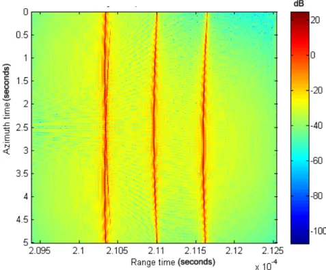
|K|Tr); a sinc function. The result is shown in figure 2.4.

Figure 2.4: Range compressed signal in the time domain

2.2. Azimuth Fourier transform

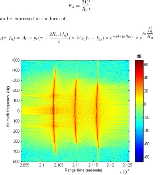
After range compression, the signal is transformed into the range-Doppler domain with the main goal of performing an efficient RCMC. This is done by doing aDFT in the azimuth direction. In this domain, the energy of scatterers at the same slant range of closest approach falls into the same cell, therefore, performingRCMC is much easier in this domain. We can see the result in figure 2.5. The resulting signal, if we do the slant range approximation for low squint cases, is:

Src(τ, fη) =A0×pr(τ −

2Rrd(fη)

c )×Wa(fη−fηc)×e

−j4πf0R0/c_×_e

jπ f_η2R0λ

2V2

(28)

2.2. AZIMUTH FOURIER TRANSFORM

The azimuth phase modulation is now shown in the last exponential term. The signal hasFM characteristics with the azimuth linear FM rate being:

Ka=

2V_r2

R0λ (2.4)

So it can be expressed in the form of:

Src(τ, fη) =A0×pr(τ −

2Rrd(fη)

−j4πf0R0/c_×_e

jπ f_η2

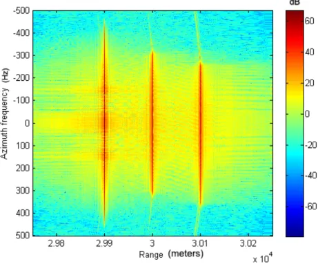
Ka (2.5)

Figure 2.5: Range compressed signal in the range-Doppler domain

A correspondence between time an azimuth frequency is established: fη = −Kaη. As we can see, the two lines representing the two scatterers which have the same slant range of closest approach have fallen in the same region of the image in the range Dop-pler domain.

If we are in a general case, in which the squint angle is not zero, we will have to calculate the Doppler centroid in order to center our spectrum at that point, because the next steps in our algorithm need to know the exact Doppler frequencies.

(29)

2.3. RANGE CELL MIGRATION CORRECTION

2.3. Range cell migration correction

It has been stated before that, due to the movement of the platform, the energy of one scatterer spreads over several range cells. In order to accomplish an effective azimuth compression without defocusing we need them to be at the same column in our matrix. This process is called Range Cell Migration Correction (RCMC). There are several ways to do this, but theRDAuses an interpolation in the range Doppler domain.

First of all we need to know the amount of RCM (Range Cell Migration) of each range cell. We know that R(η) 'R0 + (Vrη)2/(2R0) in the low squint case. So in the frequency domain:

R(f)'R0+

(V rf η/Ka)2

2R0

=R0+

(λfη)2R0

8V2

r

(2.6)

So the amount ofRCM to correct in the low squint case is: (λfη)2R0/(8Vr2). This re-presents the target displacement as a function of azimuth frequency. It is also range variant: near targets suffer more RCM.

Figure 2.6: Range-Doppler matrix afterRCMC

(30)

2.4. AZIMUTH COMPRESSION

making convolutions.

Assuming that theRCMC interpolator is applied accurately, the signal becomes:

Srcmc(τ, fη) =A0×pr(τ −

2R0

−j4πf0R0/c_×_e

jπ f_η2

Ka _(2.7)

In figure 2.6 we can see the result of applying RCMC by an interpolator. We can see that the curves describing the trajectories of the targets in the previous figures have been rectified, so the targets energy is content in a single column.

2.4. Azimuth compression

We saw in the previous section that the data has an azimuth phase modulation. We can apply a matched filter similar to the one applied to compress the data in the range direction.

In this case the filter would be:

Haz(fη) =rect( f

|K|Tr

)×e(−jπfη2/Ka) (2.8)

Figure 2.7: Final SAR image

(31)

2.5. HIGH SQUINT ANGLES

The resulting signal will be of the form:

Sac(τ, fη) =A0×pr(τ −

2R0

c )×Wa(fη −fηc)×e

−j4πf0R0/c (2.9)

Applying anIDFT in the azimuth direction completes the compression. The resul-ting signal is:

sac(τ, η) =A0×pr(τ −

2R0

c )×pa(η)×e

−j4πf0R0/c_×_ej2πfηcη (2.10)

pa is the amplitude of the azimuth impulse response, a sinc function similar topr. The target is now positioned at τ = 2R0/c and η=0, recalling thatη is relative to the time of closest approach. We can see in figure 2.7 the resulting image. The first image of the chapter —with each target placed in its position, figure 2.2— can be recognized. All the graphics shown have their module in a logarithmic scale if not stated otherwise. In this form, the variations are smaller and we can appreciate better the sidelobes of each target.

2.5. High squint angles

With the previous steps we are able to produce a focused image in a low squint scenario. If the antenna squint is higher we have to take into account other effects that are not negligible.

First of all the expression of the range equation should be substituted by a more precise one in all the previous steps.

R(η) =

q

R2₀+ (Vrη)2₌_R 0×

s

1 + (Vrη

R0

)2 ₌_R

0×D(η) (2.11)

which in the range Doppler domain is:

R(fη) =R0× s

1 + (fηλ 2Vr

)2 ₌_R

0×D(fη) (2.12)

So theRCMC should be performed taken this into account. Also the azimuth mat-ched filter has a more precise form:

Haz(fη) =rect( f

|K|Tr)×e

j4πR0D(fη)/λ (2.13)

(32)

2.6. FINAL RESULT

The filter applied in the range Doppler domain is:

Haz(fτ) =ejπfτ2/Ksrc _{where Ksrc}₌ 2V

2

rf04D3

cR0fη2

(2.14)

Figure 2.8 shows the result of applying this considerations into a scenario in which the radar antenna has20° of squint. If these corrections were not made, the target would

appear more defocused.

Figure 2.8: FinalSAR image taken with a system with squint angle

2.6. Final result

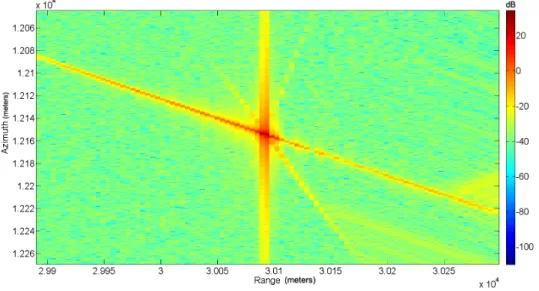
The final result of our algorithm is that we have compressed our raw signal in the range and azimuth direction, placing almost all the power of a target on its correspon-ding cell. The result can be seen in figure 2.9.

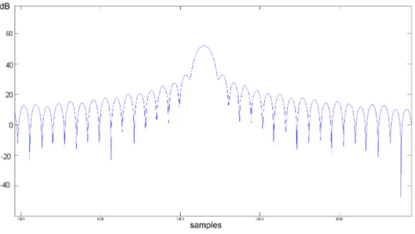
We can also extract the profiles of the target in the range and azimuth directions. Both profiles take the form of a sinc waveform, as we expected. This is because both the azimuth and the range compression lead to a sinc function at the end. We can appreciate that we have achieved a relation between the main lobe and the sidelobes larger than 20 dB. This is because we have windowed our filters.

(33)

2.6. FINAL RESULT

Figure 2.9: Zoom of the samples of a single point target

(34)

Chapter

3

MOVING TARGETS

We have seen that SAR is a coherent technique for imaging the Earth ground that relies on the principle that targets at different distances produce a different phase shift on the received signal. The radar moves along a straight line and the distance to each target varies. Taking into account the expected phase shift for each target, the radar can make an image of the ground.

If the targets are moving, their echoes do not experience the expected phase shift, so the image gets blurred and displaced. We are now going to describe the effects of moving targets in ourSAR images.

In a general scenario in which the target moves in a general direction, it gets both blurred and displaced in azimuth. This is because the movement is a combination of two instantaneous velocities, one in the range direction and the other in the azimuth direction, which lead to two different effects in the final image.

3.1. Range movement

The range movement produces a shift in the Doppler frequency which produces the displacement of the target in the azimuth direction. To illustrate this process, six dif-ferent targets with the same initial position but difdif-ferent range velocities (and with no azimuth velocity) have been simulated.

The images presented in this section are only qualitative, so the quantities of each magnitude are not important and no axes are shown.

In the raw data image (figure 3.1) we can see that initially the energy of the six targets falls into the same positions of the matrix, but as time passes they diverge in different cells. It is interesting also to observe the signal in the range Doppler domain. In figure 3.2 we can observe that targets with different velocities experience different Doppler shifts. Target three is the only one that is not moving.

(35)

3.1. RANGE MOVEMENT

Figure 3.1: Raw data matrix of the six moving targets

(36)

3.1. RANGE MOVEMENT

Figure 3.3: FinalSAR image of the six targets without filtering

If we do not filter the signal in this domain we can conserve all the targets in the final SAR image as we see in figure 3.3. So, it is not convenient to filter the image if we want to detect moving targets in the final image because we would eliminate them. Nevertheless if we decide to filter it with the goal of reducing our signal noise, we would only conserve targets with no movement, with very slow range velocities or the aliased versions of targets with high range velocities. Figures 3.4 and 3.5 illustrate this process.

Figure 3.4: Range-Doppler domain matrix of the six moving targets after filtering

(37)

3.2. AZIMUTH MOVEMENT

Figure 3.5: FinalSAR image of the six targets after filtering

3.2. Azimuth movement

On the other hand we can study targets with azimuth velocities only. The main con-sequence of this type of movement is the blurring of the target in the azimuth direction. In figure 3.6 we can see the consequences of a target moving in this direction. This effect is produced because a mismatch in the azimuthFM rate of the received signal and the one of the matched filter. The larger the speed, the larger the mismatch and therefore more defocus in the azimuth direction is caused.

Figure 3.6: FinalSAR image of a moving target with azimuth speed

3.3. Fast moving targets

(38)

3.3. FAST MOVING TARGETS

It is also interesting to observe the effects of the magnitude of the velocity; speci-fically in the range speed case. In figure 3.7 we can see the final SAR image of three targets taken during four seconds of illumination time. Target one is still, target two moves at 5 m/s and target three moves at 30 m/s. The targets have been marked in the image; in blue where they appear, and in black where they should appear.

It can be noticed that target one is correctly situated and focused. Target three is almost well focused —a certain mismatch can be appreciated— but, as expected, it has suffer an azimuth shift due to its speed. Finally the effects of fast moving targets on SAR images can be appreciated with target number two. This target follows the black line labelled with a ‘2’, but due to its speed, it travels through several resolution cells during the illumination time, so besides the azimuth shift, this target suffers a pronounced defocus. This effect is a problem when we are trying to detect fast moving targets; their energy spreads over several resolution cells and the detection is more complicated.

Figure 3.7: FinalSAR image of three moving targets with different speeds

It is interesting for certain applications to know that you have a target in your image which is moving, and even more interesting to know the real position of that target. But before trying to guess where the target is, it is important to detect it, so different techniques have been developed to try to detect the presence and the number of moving targets inSAR images.

(39)

Chapter

4

DETECTION OF MOVING TARGETS

The detection and relocation of moving targets is a desirable feature ofSARradars. They were not designed with that purpose, but in certain applications (for example military, rescue tasks, study of the flows of water, surveillance of maritime routes...) it would be very interesting to detect the position of moving targets and the parameters of that movement (velocity and direction).

With that purpose several algorithms with different approaches have been designed. This chapter is based on theory and concepts gathered from references [8], [9], [10], [11], [12], [13] and more not mentioned.

4.1. One channel techniques

These techniques only use one channel, so the signal is received only with one anten-na. There are different approaches to achieve the detection. For example: filtering the clutter region in the range Doppler domain, so only targets with large velocities remain in the image.

These techniques can be very useful for detecting targets with large radial velocities, but they are useless with slow targets, because they are masked by the clutter. For de-tecting these types of targets it is convenient to use a multichannel approach, in which several antennas are used to receive your signal.

(40)

4.2. DISPLACED PHASE CENTER ANTENNA

4.2. Displaced Phase Center Antenna

Figure 4.1: DPCA scheme. Source: [5]

Displaced Phase Center Antenna (DPCA) is a mul-tichannel technique that uses two or more antennas to obtain two or more images of the same portion of te-rrain at different instants of time. We can then fil-ter these images applying a high pass filfil-ter in or-der to obtain an image of the moving targets, era-sing the static ones. The more antennas we have, the more images and samples we have, and therefo-re we can achieve a high pass filter of higher or-der.

The high pass filter is created by adding the different images multiplied each of them by a coefficient. For exam-ple if we only have two antennas, we deduct one image from the other. If we have three images we can deduct the second one multiplied by two from the first one and after

that, add the last one. The result is an image in which we only have the moving tar-gets and the random noise, independent in each image, so now we only have to detect the moving targets. In figure 4.2 we can see a SAR image in which a random clutter has been generated along with a moving target. Figure 4.3 is the result of subtracting the corresponding image from the second channel; we can see that the target is revealed.

Figure 4.2: FinalSAR image of one single moving target masked by clutter

We can apply a threshold to the image and decide that we have a target when the module of the sample is greater than that. This approach is not good when we have se-veral types of clutter; it is more efficient to adopt an adaptive approach, with a varying threshold.

(41)

4.3. ALONG TRACK INTERFEROMETRY

Figure 4.3: Result of subtracting the images of both channels

In the Constant False Alarm Ratio (CFAR) approach [6], the value of the threshold is a function of the adjacent cells; in particular of their energy. The process to decide if a sample has a target for the CA-CFAR (cell averaging CFAR) technique is explained in the implementation section.

This CFAR technique is optimized for a scenario with clutter that can be modeled as random white Gaussian noise. There are CFAR techniques that are optimized for other types of noise, for discontinuities in the properties of the clutter or for very close targets, and depending on the statistical characterization of the clutter it would be convenient to use one or another.

4.3. Along Track Interferometry

(42)

4.3. ALONG TRACK INTERFEROMETRY

Figure 4.4:ATI scheme. Source: [5]

After that, a filter has to be applied to the interferogram. It can be a phase filter, a module filter, or a combination of both criteria; the implementation of the filter is decision of the designer. Adaptive approaches can also be made with this technique, varying the filter depending on the adjacent cells.

The filtering is done by calculating a threshold. This threshold would separate the complex chart into two different zones, the one which contains the real line would be the one corresponding to the static targets, and the other, containing the rest of the chard would be assigned to the moving targets. Every sample falling in the moving targets region would be labeled as a moving target.

(43)

Chapter

5

SAR SIGNAL SIMULATOR AND

ALGORITHM IMPLEMENTATION

Having comprehended the basic ofSARimaging and the main detection algorithms, it becomes necessary to develop a simulator to implement these techniques. This simu-lator serves as a tool to polish the algorithms prior to include them into a real system.

This simulator has been created using the software Matlab. This software allows us to implement the algorithms with a very high level programming language, so with a few lines of code you can start running very complicated algorithms; this is very useful for our purpose.

5.1. Raw data simulation

The first step of the algorithm is to create the raw data signal, captured by the radar antenna, for a specific scenario. The scenario is given in the form of several sin-gular scatterers, which represent single points of the space in which the radar signal is reflected. A scatterer is defined giving its initial position, its speed and its reflectivity. For a given scenario you can create as many scatterers as you want. Almost any object and form can be simulated by several scatterers adopting the form of the object, the more scatterers you use the more accurate is the simulated signal, but the simulation last more.

Due to the high speed of the electromagnetic waves, in the great majority of sce-narios there are only a few microseconds between the transmission of the signal and its reception, so the platform has not time to move very much during that time. To simplify the simulation, the “stop-and-go” assumption —which assumes the platform as still while the radar is waiting for the echoes— is made. This is not accurate for scenarios with faster platforms or greater delays of the signal, but in a scenario with a plane acting as platform it is a reasonable assumption.

(44)

5.1. RAW DATA SIMULATION

the contribution of each scatterer, therefore we can simulate the signal produced by each scatterer and sum them coherently just before reaching the antenna, simplifying the simulation process.

So now we only have to take into account the transmitted signal and the transfor-mations it suffers for being reflected by a certain scatterer for a given platform position: first of all the signal is attenuated because of the distance from the radar to the scat-terer, also the radiation pattern of the radar antenna filters the signal twice (once at transmission and once at reception), besides the signal, due to the unknown delay and the process of demodulation used, is phase shifted and lastly the scatterer reflects only a part of the incident electromagnetic wave.

Regarding the clutter —the background in our image, the still scatterers that are not targets—, it can be simulated in different ways. In our implementation we use two approaches. One way to do it is to simulate it as many still scatterers, at least one per resolution cell, with random reflectivity. Each scatterer tries to represent the whole signal that the scatterers present in that resolution cell would produce. This is a very slow way to produce clutter, because we have to calculate the raw data for each of these scatterers. A faster way to do it is adding some Gaussian noise to the final SAR ima-ges produced by both channels. The mean of the module of the samples of that noise should be the expected reflectivity of the clutter. This is faster because we can compute random numbers in Matlab very quickly.

For efficiency reasons the raw data signal is simulated directly in its demodulated, complex and sampled (afterA/D converter) form. We also have to limit the number of samples simulated to the segment that interests us. If we do not do so, there would be a large number of samples with zero value corresponding to the moments in which there are not any echoes arriving to our antenna.

Now we arrange each of the segments that we have selected for each 1/PRF time in one row of a matrix, obtaining the raw data matrix.

To try to simulate all the effects that happen in the physical world we can also add noise. The developed simulator adds to this matrix a white, Gaussian noise with null mean. The variance of the noise is given by the desired SNR which is defined as the ratio of the energy of all the simulated samples by the energy of all the noise samples in our matrix. After that, the desired algorithm would be applied to the simulated raw data. It has to be highlighted that clear images can be obtained by this method of simulating noise even withSNRequal to zero; this is because the RDAalgorithm filters the samples in the frequency domain, compressing the targets energy and spreading the noise.

In figure 5.1 and 5.2 we can see a simulated raw data signal with a SNR of 20 dB and the image after the algorithm has been applied. As predicted the target is clearly visible and almost no sign of noise is shown in the final image.

(45)

5.1. RAW DATA SIMULATION

Figure 5.1: Raw data signal withSNR=20 dB

(46)

5.2. RDA IMPLEMENTATION

To sum up, the steps of the simulation would be:

Define the parameters of the scenario: define the portion of terrain to image, define the radar properties (frequency, speed, initial position, the characteristics of the signal, SNR at the receptor, beamwidths of the antennas...) and the scatterers present at the scene (defining for all of them their initial position, their speed and their reflectivity).

For each 1/PRF time calculate the position of the platform and the position of each scatterer, then calculate the signal contributions of each scatterer at the receiver input, taking into account the geometry of the scenario (position of each element and the radar pointing direction) and the reflectivities, and sum each contribution to form a row in the raw data matrix.

We continue doing this to simulate for as much time as we want, updating the positions of the radar and the moving scatterers.

Finally we proceed to add the noise and the clutter, if it has not been simulated as scatterers, and we can now apply the desired algorithm to the raw-data as if it had been obtained by a real radar.

5.2. RDA

implementation

Now it is time for the SAR algorithm to act on the raw-data. The Range Doppler Algorithm (RDA) has been chosen for its implementation on our simulation. This al-gorithm has been selected because it is simple to understand and to implement. The process has already been described; here the peculiarities of this implementation of the algorithm are described.

First of all we have to make the range compression. To do so, the samples of each row are transformed into the frequency domain (making aDFT), where they are multiplied by samples of the adapted filter. Returning to the time domain (with anIDFT) we have obtained our compressed signal.

This second step is optional, but becomes necessary in scenarios with high squint angles. It is performed in the range Doppler domain. To transform our signal into this domain we have to transform each of our columns into the frequency domain (with a DFT). It is called the Secondary Range Compression (SRC), because it tries to correct the residual coupling between the range and the azimuth by doing another range compression. A filter is implemented in this domain.

After that we have to do the RCMC, which is done also in the range Doppler domain. We have to interpolate the samples of each column to correct the misa-lignment of the targets due to the movement of the platform, so an interpolator has to be implemented. The chosen way to do it has been a sinc interpolator, which is the one which shows the best performance with signals samples almost at Nyquist rates (which is likely our case). To perform this in an efficient way it has been created a matrix with only some samples of the sinc function in the form of vectors called kernels. When it is necessary a value of the sinc function, the

(47)

5.3. MULTICHANNEL SIMULATION

nearest kernel of our matrix is chosen so we do not have to evaluate the function for every interpolation.

Now we have to make the azimuth compression. We take advantage of being in the range Doppler domain to multiply each of the columns of our matrix by the adapted filter.

Finally if we perform aIDFT in order to go back to the time-time domain we can see that we have each of our targets compressed in single points.

The range and azimuth corresponding to each of the samples has to be calculated for the final representation of theSAR image.

5.3. Multichannel simulation

We have derived a process to extract a SAR image from simulated data, if we wanted to simulate the different images of multichannel radar we would have to generate multiple raw-data matrix and to apply the RDAto each of them. In our simulator the only effects that we have taken into account for the different received signals are the different positions of each of the antennas and the different random noise captured, considering negligible other effects (random variable conditions of the propagation of the signal, variations on the reflectivity...). So the steps to simulate multiple antennas would be as follows:

Simulate the scenario and simulate the received signal for one antenna applying later the algorithm as previously stated.

Simulate everything again for the other antennas but with one particularity. The image should be the same if the targets are not moving but if they are moving, that displacement should be reflected in our raw-data, so we have to simulate the scenario with a delay. This delay would be equal to the distance between the antennas divided by the speed of the platform; this is because the antennas are aligned in the along-track direction, so one antenna would be occupying the same space as the previous one when that time has passed. The noise would be different as this is a different realization, but the clutter should remain equal in both images, as it represents the non-moving background.

Finally we have obtained two (or more) images that reflect the different positions of the moving targets with the same clutter and have different noise added.

5.4. Detectors implementation

Until now we have derived a way of simulating the different signals obtained by a multichannel SAR. It is time to implement different kinds of moving target detectors to provide our radar with a GMTI mode.

(48)

5.4. DETECTORS IMPLEMENTATION

to have one sample per resolution cell. In this way, as explained in chapter 1, section 1.6, we obtain images in which each resolution cell is represented only by one sample, improving our detection performance —we would only detect in the ideal case each target one time. After performing this process, the algorithms can be applied.

5.4.1. Displaced Phase Center Antenna implementation

This detector tries to use the different images obtained to cancel the clutter present in ourSAR image as explained before. This is done by using a high pass filter. In our simulator this filter has been implemented applying the coefficients specified in this ta-ble to each of the channels. These coefficients correspond to the binomial coefficients (algebraic expansion of the powers of a binomial).

Channel N° 1 2 3 4 5 6 1 Channel No clutter supression 2 Channels 1 -1

3 Channels 1 -2 1 4 Channels 1 -3 3 -1 5 Channels 1 -4 6 -4 1 6 Channels 1 -5 10 -10 5 -1

Table 5.1: DPCA coefficients

We can see in table 5.1 that we need more than one antenna to achieve some clutter suppression. With more antennas we achieve more abrupt filters and, therefore, better clutter cancellation, but two antennas are enough to obtain very good results. It can be seen that the coefficients in each row of our table sum zero. Doing this we cancel the static samples in our image, leaving only the moving ones. We now have to apply and algorithm to distinguish our targets from the residual clutter and the signal noise, and theCFAR family of algorithms seems a very good option.

As we said in the previous section, there are severalCFAR algorithms, and each of them is optimized for a different situation. We have selected the CA-CFAR approach, because it is optimized for random white Gaussian noise and we have simulated our clutter with these characteristics.

This approach works as follows: First you select a window around your sample, then you calculate the mean energy of all the samples falling into that window without including the sample that you are analyzing and maybe the adjacent samples (the pa-rameter M specifies how many) if you think that they might be contaminated by the virtual target. After that, you multiply that by a factor (parameter T) that depends on the desired false alarm ratio, obtaining your threshold. Finally you compare your threshold with the energy of the considered cell, being able to determine if there is a target. In figure 5.3 the process is schematized.

(49)

Figure 5.3:CA-CFAR scheme. Source: [7]

This detector should be applied in our final SAR image in both directions (range and azimuth), determining that there is a moving target in the selected cell only if it has been determined in the two cases. Another implementation (which has been named DPCA-2D) calculates the threshold with the samples around our potential target, so we have to select a bidimensional window instead of two one dimensional ones.

These approaches can be considered as adaptive, because the selected threshold is a function of the adjacent cells, so it considers only the local characteristics of the image instead of global ones.

5.4.2. Along Track Interferometry implementation

In this implementation only two channels are required. One of the final images obtained is multiplied by the complex conjugate of the second one, leading to an inter-ferogram. As we said when this detector was explained, the interferogram can provide information of the movement of the target in the phase, so a filter in the form of two thresholds is applied to distinguish moving targets from static ones.

(50)

Figure 5.4:ATI detections

therefore, lowering the detection rate— then, it is multiplied by the parameter T. The root square of the result is the chosen threshold.

This process is made for each sample present in the image. Figure 5.4 is the result of plotting each of the samples and the filter in the complex plane.

As we can see almost all of the samples fall near the real line, a couple of them are at other angles. In the image we have seven correct detections, five false alarms, and four not detected targets.

This technique is not adaptive, because it bases its decisions considering the global image —it does not make local decisions— , but the technique can be adapted to create an adaptive one explained in the next section.

5.4.3. Adaptive Along Track Interferometry implementation

An adaptive approach has also been implemented. The essence of the detector is not changed at all; the only thing that is changed is the module threshold. The process is as follows: First of all we select a sample to analyze the presence of a moving target in it; we also select a bidimensional window around that sample and proceed to calculate the module threshold in the same way that we did in the non-adaptive implementation but only taken into account the samples inside our window. Finally we apply the thresholds to our sample deciding if it corresponds to a moving target or not.

(51)

This technique is presumably more efficient than the non-adaptive one, because it adapts to the different types of clutter that we will encounter within the same image. So it will give us a better performance in detecting moving targets, reaching lower false alarm ratios.

5.4.4. Combination of algorithms

One last idea to consider is the combination of algorithms. We would mark a de-tected target only if it has been dede-tected by both algorithms. With this technique we achieve better false alarm ratios; the drawback is that we may lose some targets.

(52)

Chapter

6

ALGORITHM COMPARISON

In this section it is explained how the performance of each algorithm has been measured. Monte Carlo tests have been done, simulating hundreds of different SAR images and applying the algorithms to them.

6.1. Monte Carlo

The process is as follows: A SAR image of a scenario with random moving targets, random clutter and random noise is obtained. It is important to randomize the speed, position and clutter of our images to contemplate every possible situation, so the con-clusions we derive are as general as possible.

Each of the detection algorithms is applied to the image to try to detect the targets. We can know where the targets appear in theSARimage because we know the parame-ters (speed, position, reflectivity...) of each of them, so we can check if an algorithm has succeed or not. Finally the number of false alarms, detections and not detected targets is calculated.

We perform this process as many times as we want, the more simulations we do, the more accurate we are with our conclusions of the algorithm, because we contemplate more situations and the law of large numbers comes into play. When we finish we can compute the false alarm ratio and detection ratios of each algorithm.

We can perform simulations varying the parameters of the algorithms; we can also vary the mean reflectivity of the targets, their range of speeds or the mean clutter reflectivity. This will lead to different false alarms and detection ratios, because each algorithm behaves differently in different situations.

6.2. Simulations and results

Several simulations have been made. They have been separated in simulations with low target velocities and simulations with large target velocities; this is important

(53)

6.2. SIMULATIONS AND RESULTS

cause the algorithms respond in a different way. Here, the parameters of the two imple-mented scenarios are shown.

◦ Scenario 1

Minimum target speed: 1.41 m/s (5 Km/h)

Maximum target speed: 11.7 m/s (42.12 Km/h)

Number of simulations: 10000

Mean target reflectivity: 5m2

Mean number of targets: 7 (The number of targets in each simulation follows an exponential distribution)

Range resolution: 5 m

Azimuth resolution: 0.5 m

Ground distance to center of scene: 30 Km

Scene width: 500 m

Scene length: 250 m Antenna length: 1 m

PRF 1500 Hz

Antennas separation: 1 m Simulation duration: 1 s Central frequency 9 Ghz Radar height: 1 Km Radar speed: 250 m/s Squint angle: 0 °

SNR: 30 dB

Elevation beamwidth: 180 ° Azimuth beamwidth: 1.7 °

◦ Scenario 2

Minimum speed: 11.7 m/s (42.12

Km/h) Maximum speed: 33.3 m/s (120Km/h)

The other parameters for this scenario are the same as the ones above.

Below, some simulations made in each of the scenarios with different parameters are presented. The results of each algorithm and the combination of algorithms are shown —in all of our simulations we have also combined the ATI-adaptive approach with the DPCA and the DPCA-2D—. The results caused by the combination are not commented, but it can be noticed that the false alarm ratio is always improved and the detection ratio is impaired.

6.2.1. Simulation 1 - Scenario 1, Gaussian clutter, low target velocities

These simulations have been done using the parameters specified in the scenario 1. The clutter has been simulated adding the same Gaussian noise to both channels as specified in the raw data implementation.

(54)

ATI

Angle1 = 10 (Phase threshold)

Angle2 = 1 (Samples with lower phases do not intervene in the decision on the module threshold) T = 5 (Factor of the threshold)

DPCA

M = 1 (number of neighbors not taken into account)

Window Size = 20 (Size of the selected window)

T = 50 (Factor of the threshold) DPCA-2D

T = 8000 (Factor of the threshold)

Window Size = 10 (Size of the selected window in each dimension) M = 1 (number of neighbors not taken into account)

ATI-ADAPTIVE Window Size=6 (Size of the selected window)

T = 3 (Factor of the threshold) Angle1 = 10 (Phase threshold)

Angle2 = 0 (Samples with lower phases do not intervene in the decision on the module threshold)

Table 6.1: Simulation 1 parameters

And the results for each algorithm are represented in figure 6.1:

Figure 6.1: Simulation 1 graphic results

Algorithm Detected False alarm ratio

ATI 54 % 1977×10−6

DPCA 56 % 2420×10−6

DPCA-2D 13 % 433×10−6

ATI-ADAPTIVE 68 % 3879×10−6

ATI-ADAPTIVE &DPCA 47 % 1141×10−6

ATI-ADAPTIVE &DPCA-2D 12 % 263×10−6

Table 6.2: Simulation 1 table of results

As we can see theDPCA-2D has a very low detection rate. This is because we have selected a high threshold factor T= 8000 (39 dB above the mean energy), leading to

(55)

very low detection rates and low false alarm ratios.

Regarding the ATI algorithms we can try to lower the thresholds to achieve bet-ter detection rates at expense of increasing the false alarm ratio. Taking into account these considerations another simulation has been made changing the parameters of the algorithms.

6.2.2. Simulation 2 - Scenario 1, Gaussian clutter, low target velocities

This simulation is the same as the previous one but changing the parameters used for each detector, which are represented in table 6.3. The results for each algorithm are represented in figure 6.2.

ATI

Angle1 = 10 Angle2 = 1 T = 5

DPCA

M = 1

Window Size = 10 T = 50

DPCA-2D

T = 150

Window Size = 4 M = 0

ATI-ADAPTIVE

Window Size=6 T = 2 )

Angle1 = 10 Angle2 = 1

Table 6.3: Parameters used in simulations 2 and 4

(56)

ATI 62 % 1368×10−6

DPCA 75 % 1710×10−6

DPCA-2D 64 % 5774×10−6

6.2.3. Simulation 3 - Scenario 1, clutter with scatterers, low target velocities

Other type of clutter has been tested in this simulation. Before, we were working with a clutter simulated as random Gaussian white noise added to both channels. Now we simulate it as the other way described in the raw data simulation: as still scatterers distributed around the scene. At least one scatterer per resolution cell has to be simu-lated (with random position and reflectivity) to obtain realistic results, but a density parameter has been implemented, just in case the simulation last too much. A density of 0.8 (80 % of the resolution cells have a target) has been chosen for this simulation. Different simulations were performed varying the parameters of the algorithms. One combination which obtained good results was the represented in table 6.5.

(57)

ATI

Angle1 = 10 Angle2 = 4 T = 1

DPCA

M = 1

Window Size = 10 T = 40

DPCA-2D

T = 45

Window Size = 4 M = 0

ATI-ADAPTIVE

Window Size=10 T = 1

Angle1 = 10 Angle2 = 3

Table 6.5: Simulation 3 parameters

And the results for each algorithm are represented in figure 6.3 and table 6.6.

ATI 63 % 3258×10−6

DPCA 69 % 1295×10−6

DPCA-2D 75 % 2235×10−6

(58)

we have to simulate 1292 scatterers for the clutter. The time spent simulating all the scatterers is very large and not practical, because we want to do a lot of simulations, so this has been the only simulation performed with this type of clutter.

6.2.4. Simulation 4 - Scenario 2, Gaussian clutter, high target veloci-ties

This simulation has been performed with the second scenario, the one with faster targets. It has to be noticed that the effects described in chapter 3 section 3.3 and shown in figure 3.7 occur in these simulations; therefore it has to be expected a degradation in the false alarm ratio.

The parameters used in this simulation for each algorithm are the same as the ones used in the second simulation, represented in table 6.3 and the results are expressed in figure 6.4.

It can be appreciated in general a degradation of the results. This is because the target’s energy has spread among several resolution cells, therefore, using our previous detectors, there is no way to say that the detections are several targets or one single fast target. Before applying the algorithms we state that each target is in the cell in which it has more energy in the finalSARimage. When we apply the detection algorithms to that cell, the adaptive threshold is increased, because of this leakage of energy to other cells, so it is possible that we do not detect targets in any cell. This is what happens in theDPCA-2D algorithm, in which both the false alarm ratio and the detection ratio have been lowered by a lot.

In theATI algorithms, we can see that the detection rate has remained almost the same. This is because the adaptive threshold in less important in this algorithm, being more important the phase threshold. We can also see that the false alarm ratio has been increased.

A solution to the problem of the increased threshold would be to increase the para-meter M of the algorithms —the number of neighbors not taken into account to calculate it— so we do not take into account the contaminated cells. With this approach we take the risk of not being as adaptive as we could, because these neighbors are the ones which give us more information. This could lead to several detections for one target, as it occurs in theATI algorithms.

A solution of the problem of several detections for one target is to consider the detected target and the adjacent detections as one single target applying clustering techniques. By doing this we are risking to treat two near moving targets as one single moving target.

(59)

ATI 68 % 3755×10−6

DPCA 63 % 3704×10−6

DPCA-2D 13 % 627×10−6