Contact map prediction based on cellular automata and protein folding trajectories

Texto completo

(1)Contact Map Prediction based on Cellular Automata and Protein Folding Trajectories. Nestor Milciades Diaz Mariño. Supervisor: Ph. D. Irene Tischer. Thesis submitted for the degree of Doctor in Engineering – Emphasis Computing Science. Universidad del Valle Engineering Faculty School of Systems Engineering and Computation October 2019.

(2) Copyright 2019 Nestor Diaz.

(3) Abstract. In Structural Bioinformatics, it is necessary to know the protein’s tertiary structure because its specific shape is central in its interaction with binding molecules. Being experimental tertiary structure determination a highly expensive process, computational protein structure prediction becomes an alternative option aimed toward cost and technical limitations reduction. In the last decade, residue-residue protein contact prediction (PCP) has taken broad consideration. Currently, PCP has become a common subtask of computational structure prediction. Residue-residue interactions can constraint the space. of. possible. protein. conformations,. improving. protein. structure. determination. Despite the recent improvements in PCP, the high rate of false positive predicted contacts hinders the applicability of existing PCP tools. To reduce the false positive rate in PCP, we developed a novel approach based on cellular automata (CAs), which determines residue-residue contacts that are likely to be actual contacts. Our approach exploits the local interactions found in protein contact maps and the iterative refinement provided by CAs. Our CAs were identified using a parallel genetic algorithm which used for training the PSICOV data set (150 proteins). To benchmark our approach, we used the CASP12 data set (Critical Assessment of Techniques for Structure Prediction, year 2016). Our best CA outperformed the ten PCP tools compared in the benchmark. However, a more.

(4) detailed analysis using non-parametric Friedman’s statistical test revealed that our tool does not excel the performance of prominent PCP tools such as MetaPSICOV and RaptorX-Contact. Although our CA-based approach for PCP was successful, the precision for long-range contacts (sequence separation > 24 amino acids) was hard to improve. To enrich local interactions, we proposed a multiclass contact map representation that can improve long-range PCP. Our multiclass contact map was obtained using a large-scale comparison of decision trees. The next step to follow is to reformulate our CA-based approach to incorporate multiclass contacts and repeat the overall process to obtain a new PCP tool..

(5) Table of Contents. Table of Contents ................................................................................................................. i List of Tables .......................................................................................................................v List of Figures .................................................................................................................... vi List of Annexes .................................................................................................................. ix Chapter I. Introduction .........................................................................................................1 1.. Thesis Overview ..........................................................................................5. 2.. References ....................................................................................................7. Chapter II. Referential Framework ......................................................................................9 1.. Glossary .....................................................................................................10 Inter-Residue Contact. ...................................................................10 Contact Range. ...............................................................................10 Sequence Separation. .....................................................................11 Contact Map. ..................................................................................12 Reference Databases. .....................................................................13 Template Based Modeling and Prediction. ....................................13 Free Modeling. ...............................................................................13 Correlated Mutation. ......................................................................13 Direct Coupling Analysis. ..............................................................15 Mutual Information. .......................................................................16 Critical Assessment of Protein Structure Prediction (CASP). .......16. i.

(6) 2.. State of the Art ...........................................................................................17 2.1. Evaluation Protocol in CASP.........................................................17. 2.2. Performance Measures in CASP12................................................18. 2.3. Target Proteins in CASP12 ............................................................21. 2.4. Top Predictors in CASP12 .............................................................23 MetaPSICOV .................................................................................24 DeepFold_ Contact, iFold_1, and naive ........................................27 RaptorX-Contact ............................................................................28 MULTICOM-CONSTRUCT .........................................................29 PConsC31 and PCons-net ..............................................................30 FALCON_COLORS ......................................................................32 IGBTeam........................................................................................32. 3. Cellular Automata and PCP .......................................................................33. 4. Conclusions ................................................................................................36. 5. References ..................................................................................................37. Chapter III. GACAI-PCP: Cellular Automata based Tool for Contact Map Prediction ...44 Abstract ......................................................................................................44 1.. Introduction ................................................................................................44. 2.. Materials and Methods ...............................................................................47 2.1.. Initial Conditions Dataset ..............................................................47. 2.2.. Cellular Automata Identification Framework ................................49 2.3. Genetic Algorithm for Identification of CAs that evolve Contact Maps .................................................................................49. ii.

(7) 2.4.. Density Classification Task as Benchmark for GACAI-PCP ........51. 3.. Discussion ..................................................................................................52. 4.. Conclusion .................................................................................................55. 5.. References ..................................................................................................56. Chapter IV. Contact Map Prediction based on Cellular Automata ....................................58 Abstract ......................................................................................................58 1.. Introduction ................................................................................................59. 2.. Materials and Methods ...............................................................................63. 3.. 2.1.. Databases and Training Data Sets..................................................63. 2.2.. Initial Conditions Generation.........................................................64. 2.3.. Standard Tools ...............................................................................72. 2.4.. CA-based PCP Method Description ..............................................72. Prediction Results ......................................................................................76 3.1.. Validation Data Set ........................................................................76. 3.2.. PCP-CA Model 1 ...........................................................................76. 3.3.. Prediction Example using PCP-CA ...............................................79. 3.4.. PCP-CA Evaluation .......................................................................80. 4.. Discussion ..................................................................................................82. 5.. Conclusion .................................................................................................84. 6.. References ..................................................................................................85. Chapter V. Multiclass Protein Contact Maps ....................................................................89 Abstract ......................................................................................................89 1.. Introduction ................................................................................................90. iii.

(8) 2.. 3.. Methods......................................................................................................92 2.1. Contact Ranges Combinations .......................................................94. 2.2. Datasets Generation .......................................................................96. 2.3. Decision Trees Building and Evaluation .......................................97. 2.4. Top Models Selection ....................................................................98. 2.5. Top Decision Trees Comparison .................................................100. Results ......................................................................................................104 3.1. Contact Refinement .....................................................................105. 4. Conclusions ..............................................................................................108. 5.. References ................................................................................................109. Chapter VI. Conclusions and Future Work......................................................................112 References ............................................................................................................115. iv.

(9) List of Tables. Chapter II. Referential Framework Table 1. Consolidated results in CASP12 official residue-residue contact predictions. .. 20 Table 2. Top 10 predictors CASP12 by an average of performance measures. ............... 25 Chapter IV. Contact Map Prediction based on Cellular Automata Table 1. All performance measures for predictors MetaPSICOV and RaptorX-Contact. 71 Table 2. PCP-CA rule description. ................................................................................... 77 Table 3. Precision by target/predictor CASP12 top 10 plus PCP-CA, for full list contacts and medium/long range sequence separation. .................................................................. 81 Table 4. Average precision for all predictors at several sizes of list of contacts for all target in CASP12. ............................................................................................................. 83 Chapter V. Multiclass Protein Contact Maps Table 1. Average rankings of DTs for top contact range combinations. ........................ 103 Table 2. MCC for each protein trajectory in the test set for contact refinement. ........... 107 Table 3. Wilcoxon test for contact refinement comparison. ........................................... 108. v.

(10) List of Figures. Chapter I. Introduction Figure 1. Project breakdown structure. ................................................................................3 Chapter II. Referential Framework Figure 1. Native structure for protein 1vii. ........................................................................12 Figure 2. Four contact maps for protein 1vii, contact range 8 Å. ......................................14 Figure 3.Native structure and contact map for protein 1vii. ..............................................15 Figure 4. CASP12 PCP targets. First half. .........................................................................23 Figure 5. CASP12 PCP targets. Second half. ....................................................................24 Figure 6. Proposed pipeline for PCP training and CA-based PCP prediction. ..................37 Chapter III. GACAI-PCP: Cellular Automata based Tool for Contact Map Prediction Figure 1. RaptorX-Contact predicted contact map and actual contact map for target protein T0900 (CASP12). ..................................................................................................47 Figure 2. Pipeline for the generation of the dataset of initial conditions. ..........................48 Figure 3. Genetic Algorithm Process for CA identification. .............................................50 Figure 4. Examples of Moore’s CA neighborhood. ...........................................................53 Figure 5. Performance of the five CAs on the CASP12 evaluation dataset. .....................53 Figure 6. Dominance graph analysis with statistical significance comparison by Friedman’s test and post-hoc Nemenyi’s test. ...................................................................55 Chapter IV. Contact Map Prediction based on Cellular Automata. vi.

(11) Figure 1. MetaPSICOV2 predicted contact and actual contact map for target protein T0866 (CASP12). ..............................................................................................................62 Figure 2. Dominance graph for top 10 contact predictors in CASP12, FM targets, top L/2 contacts, full + medium sequence separation, and precision as performance measure. ....67 Figure 3. Dominance graph for top 10 contact predictors in CASP12, FM targets, top L contacts, full + medium sequence separation, and precision as performance measure. ....68 Figure 4. Dominance graph for top 10 contact predictors in CASP12, FM targets, FL, full + medium sequence separation, and precision as performance measure. ..........................70 Figure 5. Dominance graph for top 10 contact predictors in CASP12, FM targets, FL, full + medium sequence separation, and accuracy as performance measure. ..........................71 Figure 6. Pipeline for a conventional PCP approach. ........................................................74 Figure 7. Pipeline for CA-based PCP. ...............................................................................75 Figure 8. PCP-CA Neighborhood. .....................................................................................76 Figure 9. Examples of transitions in the PCP-CA rule. .....................................................78 Figure 10. Contact map predicted by PCP-CA / MetaPSICOV2 for CASP12 target protein T0891. ....................................................................................................................79 Figure 11. Dominance graph for top 10 contact predictors in CASP12 plus PCP-CA for CASP12 targets, full list of contacts predicted, full + medium sequence separation, and precision as a performance measure. .................................................................................82 Chapter V. Multiclass Protein Contact Maps Figure 1. Method RoadMap. Three phases, inputs/outputs, and processes. ......................94 Figure 2. EM clustering of DTs performance measures for 413 contact ranges combinations. .....................................................................................................................99. vii.

(12) Figure 3. Frequencies by rule ranges in the dataset. ........................................................101 Figure 4. Nemenyi’s test results.......................................................................................103 Figure 5. The rule in a 2-state contact map vs. 4-state contact map for Model 1. ...........104 Figure 6. Average results for contact map refinement. ....................................................106. viii.

(13) List of Annexes. Annex 1: Generic framework for mining cellular automata models on protein-folding simulations (Published Paper). Annex 2: GACAI-PCP: Cellular Automata based Tool for Contact Map Prediction (Published Paper). Annex 3: Data mining approach to improve protein contact maps (Submitted Paper). Annex 4: Mining Stochastic Cellular Automata to Solve Density Classification Task in Two Dimensions (Submitted Paper).. ix.

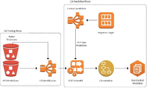
(14) Chapter I. Introduction. Proteins are a primary component of the vital processes for all kind of living beings, including the human being. The native structure of a protein determines the biological function that it will fulfill, and for this reason, it is necessary to know this structure. For several decades, multidisciplinary researchers have been working on methods that allow predicting or identifying a near-native structure for a protein from its amino acid sequence only. Despite all existing approaches to protein structure prediction, the problem remains unsolved, given the low quality of predicted structures especially for proteins with few homologs. In the last decade, residue-residue contacts have become a common source of information about constraints in the space of possible conformations(Ovchinnikov et al., 2018). Contacts stabilize protein folds, at all levels including short range interactions as well as long range. The high rate of false contacts that predictors usually produce (Kosciolek & Jones, 2014), is the topic addressed in our approach. Our solution exploits the mechanism based on local information that cellular automata (CAs) provide. Our CA-based approach improves the performance of residue-residue contact prediction. CAs fit in the task related to improving the full list of contacts predicted because they can generate global coordination from local information only. CAs do not require global control and computation is done from a set of local transitions.

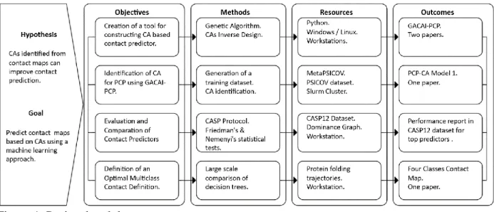
(15) defined in a small window around each cell of the contact map. Chapter II introduces the reader to the concepts related to protein contact map prediction (PCP) and CA. A CA in 2D arranges information in a matrix similar to a contact map. However, they provide two complementary features: 1) a set of local transitions, called rule; 2) and the capability to evolve the initial matrix state using the CA rule. Our approach requires to identify the rule of a CA able to evolve an initial predicted contact map to a more realistic one. In this thesis, we develop the hypothesis that CAs can improve predicted contact maps. However, the CAs modeling must be accomplished by a machine learning approach because the mechanism able to evolve a predicted contact map into a closer to the real one, is unknown. In the context of our approach, the main goal was to predict contact maps with better accuracy. As mentioned above, one current issue in protein contact prediction (PCP) is the high proportion of false positives (FP), so that our approach was focused in the reduction of FP to improve accuracy. In Figure 1, we use a project breakdown structure (Becker et al., 2014) to depict how the thesis development was structured. To accomplish our main goal of predicting contact maps, we developed four specific objectives, and for each one, we mention in Figure 1 the methods, the resources, and the outcomes. The first specific objective was the implementation of a genetic algorithm (GA) that models CAs for PCP. The GA task is to design a CA from the information provided by pairs of initial configurations (IC) – final configurations (FC), this kind 2.

(16) of approach is called inverse design (Back et al., 2005). An IC is the initial state or initial prediction, and the FC is the desired final global state where the GA must identify the CA rule that evolves the IC to the desired state or improved prediction. We describe the software architecture of our approach in (Díaz & Tischer, 2016) (Annex 1 “Generic framework for mining cellular automata models on proteinfolding simulations”). The specific details of the GA for PCP are described in Chapter III “GACAI-PCP: Cellular Automata based Tool for Contact Map Prediction” and was published in (Diaz & Tischer, 2019).. Figure 1. Project breakdown structure.. The thesis was organized in a way that objectives are accomplished through the methods, which utilize the resources to achieve the outcomes that support the hypothesis about the use of CAs in PCP. Further, we showed that the software framework could solve diverse problems related to the inverse design of CAs, such as the density classification task. 3.

(17) (DCT) (De Oliveira, 2014). Our results for DCT are described in Annex 4 “Mining Stochastic Cellular Automata to Solve Density Classification Task in Two Dimensions.” The second specific objective involved the generation of the training dataset comprised of ICs obtained from MetaPSICOV (Buchan & Jones, 2018) predictions and their native contact maps (desired final state). MetaPSICOV was the best option, as we concluded through the statistical comparison of the top predictors that we describe in Chapter III. The set of protein sequences used for training was the one described in (Jones et al., 2012). The identification of CAs is a computationally expensive task; therefore, it was necessary to run the GA in a highperformance computing cluster. The third specific objective aims for the evaluation of PCP results by following the CASP (Critical Assessment of Protein Structure Prediction) protocol (Monastyrskyy et al., 2011). The validation dataset contains the target proteins published for CASP round 12 (CASP12). For a more detailed comparison of our predictor and the CASP top-10, we propose a graphical tool called Dominance Graph that displays the rankings and dominance relationships for predictors in an all vs. all comparison. The details of the results and the comparison with the top-10 predictors for the best identified CA are described in Chapter IV. The last specific objective opens the way to a complementary approach in contact map prediction. The binary definition of contacts in traditional approaches is an inherent source of complexity for PCP. The binary definition (contact / no – 4.

(18) contact) implies that several inter – secondary structure interactions are hard to predict because these are scarce in the contact map. As a complement to the work with binary contact maps, we developed a large – scale comparison of multiclass contact maps that convey richer information for scarce contacts. These results were submitted to the Journal of Machine Learning Research under the title “Data mining approach to improve protein contact maps.” We are currently developing an algorithm to generate ICs for optimal multiclass contact map representation because none of the existing predictors is compatible with our proposed definition. In this thesis, we explored the use of CAs to improve PCP, and satisfactorily proved that its characteristic emergent global coordination was helpful to reduce the excessive proportion of FP that the state of art predictor MetaPSICOV produces.. 1.. Thesis Overview. Chapter II starts with a description of the relevant concepts in PCP and CAs. Then we survey the results for PCP in CASP12, we select and describe the top-10 predictors. The chapter concludes, showing the relationship between CAs and PCP. Chapter III describes our approach for inverse design of CAs, the CA definition we used, and preliminary results. Finally, we compare our identified CA for PCP with other CAs that use traditional neighborhoods instead of the machine learning designed neighborhood of our approach.. 5.

(19) In Chapter IV, we describe, analyze, and survey our best CA in the context of the top-10 predictors defined in Chapter II. In particular, we focused our analysis on Friedman’s framework and Nemenyi’s tests and dominance graphs. Chapter V reports our approach to find an optimal definition of multiclass contact map. Our optimal multiclass definition was selected from a set of plus four – hundred combinations of contact ranges. We evaluated each candidate multiclass definition using decision trees and performance measures adapted for this problem. Finally, Friedman’s and Nemenyi’s tests allowed us to select an optimal definition. In Chapter VI, we resume the main contributions of this thesis and indicate further work. Annex 1 contains our published paper “Generic framework for mining cellular automata models on protein-folding simulations,” which describes the software architecture at the core of our approach. Annex 2 comprises our published paper “GACAI-PCP: Cellular Automata based Tool for Contact Map Prediction.” GACAI-PCP is our GA designed to identify CAs for PCP. In Annex 3, we include our submitted paper “Data mining approach to improve protein contact maps,” which describe the methods and results of our approach for multiclass contact map definition.. 6.

(20) Annex 4 contains our submitted paper “Mining Stochastic Cellular Automata to Solve Density Classification Task in Two Dimensions,” which describes our solution to DCT that allowed us to tune the parameters for GACAI-PCP.. 2.. References. Back, T, Breukelaar, R, & Willmes, LBT-UPP. (2005). Inverse Design of Cellular Automata by Genetic Algorithms: An Unconventional Programming Paradigm. In Unconventional Programming Paradigms (pp. 161–172). Springer. Retrieved from http://dx.doi.org/10.1007/11527800_13 Becker, M, Schütt, B, & Amini, S. (2014). Proposal Writing for International Research Projects: A Guide for Teachers. Buchan, DWA, & Jones, DT. (2018). Improved protein contact predictions with the MetaPSICOV2 server in CASP12. Proteins: Structure, Function and Bioinformatics. http://doi.org/10.1002/prot.25379 De Oliveira, PPB. (2014). On Density Determination With Cellular Automata : Results, Constructions and Directions. Journal of Cellular Automata, 9(5–6), 357–385. Diaz, N, & Tischer, I. (2019). GACAI-PCP : Cellular Automata based Tool for Contact Map Prediction. In 17th LACCEI Latin American and Caribbean Conference for Engineering and Technology (pp. 1–5). Díaz, N, & Tischer, I. (2016). Generic framework for mining cellular automata models on protein-folding simulations. Genetics and Molecular Research, 15(2), 1–16. http://doi.org/10.4238/gmr.15028654 Jones, DT, Buchan, DW a, Cozzetto, D, & Pontil, M. (2012). PSICOV: precise structural contact prediction using sparse inverse covariance estimation on large multiple sequence alignments. Bioinformatics (Oxford, England), 28(2), 184–90. http://doi.org/10.1093/bioinformatics/btr638 Kosciolek, T, & Jones, DT. (2014). De novo structure prediction of globular proteins aided by sequence variation-derived contacts. PLoS ONE, 9(3), 1–15. http://doi.org/10.1371/journal.pone.0092197 Monastyrskyy, B, Fidelis, K, Tramontano, A, & Kryshtafovych, A. (2011). Evaluation of residue–residue contact predictions in CASP9. Proteins, 79(Suppl 10), 119–125. http://doi.org/10.1002/prot.23160.Evaluation. 7.

(21) Ovchinnikov, S, Park, H, Kim, DE, DiMaio, F, & Baker, D. (2018). Protein structure prediction using Rosetta in CASP12. Proteins: Structure, Function and Bioinformatics, 86(July 2017), 113–121. http://doi.org/10.1002/prot.25390. 8.

(22) Chapter II. Referential Framework. Protein contact prediction (PCP) is a research area which originates at least four decades ago. The first approach that exploits the benefits of contact prediction is the one described in (Tanaka & Scheraga, 1975). Tanaka and Scheraga propose a 3-step algorithm for protein folding, where each step incorporates information related with short, medium and long contact ranges, respectively. Later, Gromiha and Selvaraj make an extended review (Gromiha & Selvaraj, 2004), where they consolidate several decades of knowledge about inter-residue contacts and their relevance in protein structure studies. Nowadays, an important quantity of research groups is working in PCP, some in standalone predictors and others in pipelines of native protein structure predictors where PCP has an important role. Two main approaches allow classifying the best contact predictors (Sun, Huang, Wang, Zhang, & Shen, 2015): mutual information (MI) and evolutionary coupling (EC). Since 1996, the Critical Assessment of Structure Prediction (CASP) has given special attention to PCP in its biennial competition (Monastyrskyy, D’Andrea, Fidelis, Tramontano, & Kryshtafovych, 2015).. After several years of. development, EC has become perhaps the approach with the most significant improvements in the CASP competition..

(23) Even though the improvement in average precision is vast, PCP requires further advancement. In CASP12 (2016), the performance was around twice as good as the results in CASP10 (2014), but the overall precision is still under 50% (Schaarschmidt, Monastyrskyy, Kryshtafovych, & Bonvin, 2017). In this thesis, we propose and test some novel algorithms based on cellular automata which allow us to improve PCP precision by adding a new prediction layer to the results of wellknown efficient predictors (e.g., MetaPSICOV (Buchan & Jones, 2018), PSICOV (Jones, Buchan, Cozzetto, & Pontil, 2012), and EvFold (Morcos et al., 2011)). Our approach uses cellular automata as the core for machine learning of rules for PCP refinement. In this chapter, we describe the conceptual framework for PCP (as glossary) in the section 1. We describe the state of the art in section 2 and a statistical analysis of contact predictors performance in section 3. In section 4 we describe how PCP is related to cellular automata. Finally, we draw conclusions in section 5.. 1. Glossary Inter-Residue Contact. The inter-residue contact defines the closeness between a pair of residues of a protein by specifying a contact range. It allows identifying structural characteristics of a tertiary structure of a protein. Inter-residue contact is synonymous of residue-residue contact (RRC). Contact Range. The contact range is generally a sphere placed in an atom of a residue’s backbone and if the same atom of another residue of the protein is found 10.

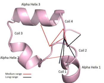
(24) inside this sphere the two residues are in contact. In PCP, predictors use carbon alpha (Cα) or carbon beta (Cβ) as reference atoms for contact analysis. The common contact range is 8 Å, and for CASP evaluation, the reference atom is the Cβ (Cα for glycine). In some cases, the contact range may also be based on the centroid of the residue or the mass center of the side chain. Sequence Separation. In PCP, the sequence separation between a pair of residues is a relevant factor in the precision evaluation because medium and long ranges are the hardest targets for prediction, although they are crucial for providing structural constraints (Monastyrskyy et al., 2015). For evaluation purposes there are three sequence separation ranges (Holland, Pan, & Grigoryan, 2018): short-range, for sequence separation greater than five and smaller than twelve residues; mediumrange, for separation greater than eleven and below twenty-four residues; and longrange separation for pairs of residues with separation above twenty-three. PCP performance evaluation excludes sequence separation inferior to six residues because contacts at this range are situated mostly inside secondary structure elements (Monastyrskyy, D’Andrea, Fidelis, Tramontano, & Kryshtafovych, 2014). In Figure 1 we show examples of contacts for protein 1vii, at medium and long range separations. In Figure 1, medium-range contacts define contacts between secondary structure elements: Coil 1 – Alpha helix 2; Coil 2 – Alpha helix 3; and Coil 2 – Coil 4. At long-range sequence separation contacts appear for Coil 1 – Coil 4 and Coil 2 – Coil 4.. 11.

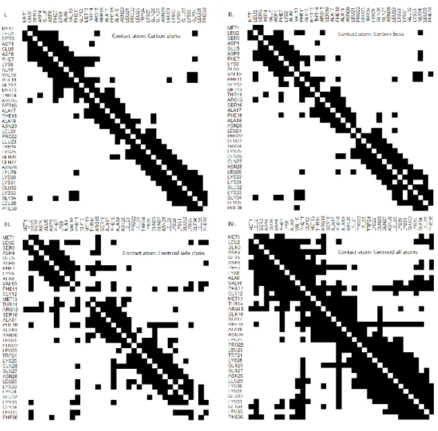
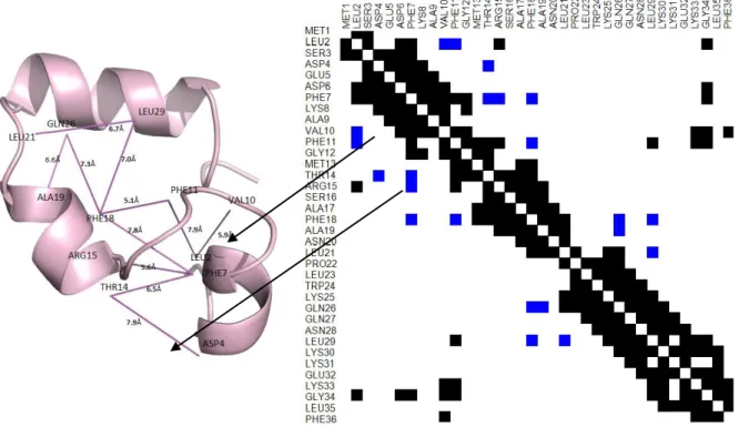
(25) Figure 1. Native structure for protein 1vii. The figure displays contacts in the contact range 8 Å for medium and long-range sequence separation. Lines indicate contacts (i.e., gray for medium-range and black for long-range). Contact Map. A contact map (CM) is a binary matrix that in row i denotes which residues of the protein are in contact range of residue i. In Figure 2, we display four contact maps for protein 1vii. This protein has a sequence of thirty-six amino acids, so its contact map is a binary matrix of size 36 × 36. Each panel in Figure 2 is a contact map that exemplifies the differences between four common definitions of contact range. Panels I and II of Figure 2, based on the Cα and Cβ atoms, respectively, are among the more popular contact range definitions. Currently, the de facto standard is the contact range definition using Cβ atoms and a threshold of 8 Å, because the predictors that participate in CASP competitions, or that at least use CASP targets and evaluation methodology as a benchmark, require to use it. In Figure 3, we show the Cβ contact map at 8 Å threshold for protein 1vii and its 3D native structure. In the native structure, residues in contact are shown linked by a straight line. Arrows in Figure 3 connect contacts for residues VAL10-LEU2 and THR14-ASP4, whose contact distance is 5.9 Å and 7.9 Å, respectively. 12.

(26) Reference Databases. Reference databases are sets of protein sequences that are used commonly in sequence analysis in PCP. Some reference databases are: PDB70 that is constructed from PSI-BLAST (Altschul et al., 1997) alignments of sequences extracted from the Protein Data Bank (PDB) with sequence similarity inferior to 70%; Uniref100 (Suzek, Wang, Huang, McGarvey, & Wu, 2015) that provides clusters of sequences extracted from UniProt Knowledgebase (Bateman et al., 2017) where of a number of repeated subsequences, only one unique sequence is stored to avoid redundancy. Uniref70, Uniref50 and Uniref20 contain the same sequences as Uniref100 but they are grouped at 70%, 50% and 20% of sequence identity. Template Based Modeling and Prediction. Some protein structures are modeled using as initial structure another protein structure. In prediction, many predictors require homolog structures to make a precise approximation of the desired structure. Free Modeling. Free modeling (FM) is a category of prediction used to indicate that a protein lacks a template or homolog structure to be used in structure prediction or any other kind of analysis. Prediction in the FM situation is hardest because Multisequence Alignments (MSAs), sequence-related data and local structure information provide important support for prediction. Correlated Mutation. Correlated Mutation is one of the most import concepts for the current success of contact prediction. The idea behind it is that there is a relationship between sequence mutations and structure, where a mutation drives to a correlated mutation because of physical constraints (Göbel, Sander, Schneider, & Valencia, 1994). Several methods integrate this concept and are categorized into two 13.

(27) main approaches: Direct Coupling Analysis (DCA) and Mutual Information (MI) explained next.. Figure 2. Four contact maps for protein 1vii, contact range 8 Å. Panel I. Distances were calculated for atom Cα of each residue pair. Panel II. Distances were calculated for atom Cβ of each residue pair. Panel III. Distances were calculated for the centroid of the residue side chain for each residue pair. Panel IV. Distances were calculated for the centroid of all the residue atoms for each residue pair.. 14.

(28) Figure 3. Native structure and contact map for protein 1vii. Contacts with a sequence separation greater than six residues and below 12 residues are shown in blue. Direct Coupling Analysis. DCA is a method for extracting information from sequence related data (Morcos et al., 2011). DCA allows inferring contacts based on amino acid composition at some sites of the protein sequence. DCA is one of the main approaches used by successful predictors. This kind of approach is useful, when it is able to discern where correlations are caused by direct relationships between amino acids and not by indirect inference. Message-passing DCA (mpDCA) is an important example of the DCA category. mpDCA locally uses MI and later applies a statistical model that incorporates frequency of amino acids at specific positions and direct couplings for those amino acids (Weigt, White, Szurmant, Hoch, & Hwa, 2009). mpDCA implements a message-passing approach to reduce computational complexity, but it is still an expensive method. Mean field DCA (mfDCA) is a. 15.

(29) computationally more efficient approach for DCA (Morcos et al., 2011). mfDCA reduces the computational cost by using analytical methods instead of the iterative one used in mpDCA. mfDCA is implemented by the open source Freecontact (Kaján, Hopf, Kalaš, Marks, & Rost, 2014). Freecontact offers an additional implementation for PSICOV (Jones et al., 2012), which is a DCA based method that uses sparse inverse covariance based on the lasso concept for neighborhood selection in sparse matrices (Meinshausen & Bühlmann, 2006). Other approaches such as plmDCA (Ekeberg, Lövkvist, Lan, Weigt, & Aurell, 2013), GREMLIN (Kamisetty, Ovchinnikov, & Baker, 2013) and CCMpred (Seemayer, Gruber, & Söding, 2014), include pseudolikelihood optimization as the core to avoid spurious indirect correlations. Mutual Information. Mutual Information (MI) (Martin, Gloor, Dunn, & Wahl, 2005), implements the concept that the identity of an amino acid in a position is able to predict which amino acid will be in another position. We mention two approaches for MI, row-column weighting (RCW) (Gouveia-Oliveira & Pedersen, 2007) and average product correction (APC) (Dunn, Wahl, & Gloor, 2008). Critical Assessment of Protein Structure Prediction (CASP). CASP is a well-established biennial competition that focuses on diverse problems in the field of protein structure. In its website (predictioncenter.org), there is information about all competitions held since 1994 (CASP1). Currently, CASP develops five prediction categories: template-based modeling, ab-initio modeling, contact prediction, refinement, and data assisted modeling. In the PCP category, predictors are applied to a protein sequences dataset of unknown structures, and assessors, chosen. 16.

(30) specifically for each competition, perform the evaluation. The evaluation protocol implies to select a top of residues pairs in contact. The top may be selected in dependence of the length (L) of the protein sequence. Evaluators commonly use the top 10, top L/5, top L/2, L and full list (FL) of predicted contacts to assess a predictor. To differentiate best predictions, the result for each pair of residues in contact must have a probability for such contact, which is defined by the predictor itself. Higher probability indicates a better likelihood for that pair of residues to be in contact in the native structure.. 2. State of the Art In this section, we describe and compare the top contact predictors using the results of CASP12 because this round is the last one with full results published until now. The next round of the competition (CASP13) is scheduled to run from April 2018 to December - 2018 and the full results will be published later.. 2.1. Evaluation Protocol in CASP As predictors based on machine learning advance in quality performance, the. CASP evaluation protocol includes measures that are very common in machine learning. Precision, recall, Matthews correlation coefficient (MCC) and area under the precision-recall curve (AUC_PR) were used in CASP11 (Kryshtafovych, Monastyrskyy, & Fidelis, 2016). Predictors are evaluated in two ways: reduced list (RL) and full list (FL) (Monastyrskyy et al., 2015). RL evaluation ensures that all. 17.

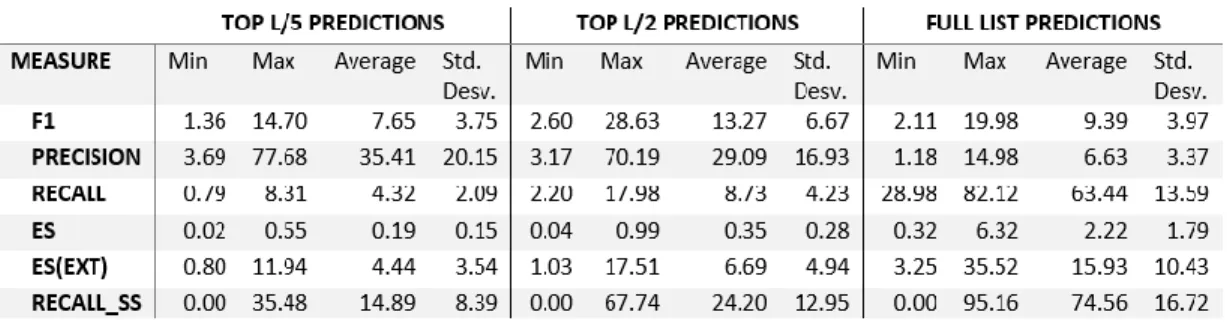
(31) predictors are assessed on the same quantity of contacts. The typical RL sizes are top-5, top-10, top L/5, top L/2, top L and top 2L (Adhikari, Nowotny, Bhattacharya, Hou, & Cheng, 2016), where L is the length of the protein sequence.. 2.2. Performance Measures in CASP12 The performance measures that evaluators selected in CASP12 were:. precision (Equation 1), harmonic mean (F1) (Equation 3), recall (Equation 2) and a pair of measures for entropy: ES (Equation 4) and ES_ext (Equation 4). Entropy measures try to capture the dispersion of predicted contacts along the overall structure (Schaarschmidt et al., 2017). Alternative adaptations of precision, F1 and recall that try to incorporate the probability associated for a predictor to each RRC predicted were also included. Being based on probabilities, these measures are skewed by the training data and the scoring method used for each predictor, so we are excluding those measures in our analysis. This topic was addressed previously by Jinbo Xu from the RaptorX-Contact team (S. Wang, Sun, & Xu, 2018) in a Web entry. (http://ttic.uchicago.edu/~jinbo/WhyF1probIsIncorrect.htm,. November 2018). 𝑇𝑃. 𝑝𝑟𝑒𝑐𝑖𝑠𝑖𝑜𝑛 = 𝑇𝑃+𝐹𝑃 , 𝑇𝑃: 𝑇𝑟𝑢𝑒 𝑝𝑜𝑠𝑖𝑡𝑖𝑣𝑒𝑠; 𝐹𝑃: 𝐹𝑎𝑙𝑠𝑒 𝑝𝑜𝑠𝑖𝑡𝑖𝑣𝑒𝑠. 𝑟𝑒𝑐𝑎𝑙𝑙 = 𝐹1 =. 𝑇𝑃 𝑃. , 𝑃: 𝑁𝑢𝑚𝑏𝑒𝑟 𝑜𝑓 𝑐𝑜𝑛𝑡𝑎𝑐𝑡𝑠 𝑖𝑛 𝑡ℎ𝑒 𝑝𝑟𝑜𝑡𝑒𝑖𝑛.. 2×𝑝𝑟𝑒𝑐𝑖𝑠𝑖𝑜𝑛×𝑟𝑒𝑐𝑎𝑙𝑙 𝑝𝑟𝑒𝑐𝑖𝑠𝑖𝑜𝑛+𝑟𝑒𝑐𝑎𝑙𝑙. 𝐸𝑆 = 100 ×. (3). 𝐸𝑛𝑡𝑟𝑜𝑝𝑦|0−𝐸𝑛𝑡𝑟𝑜𝑝𝑦|𝐶 𝐸𝑛𝑡𝑟𝑜𝑝𝑦|0. (4). 18. (2). (1). visited:.

(32) 𝐸𝑛𝑡𝑟𝑜𝑝𝑦|0: 𝑒𝑛𝑡𝑟𝑜𝑝𝑦 𝑜𝑓 𝑡ℎ𝑒 𝑝𝑟𝑜𝑡𝑒𝑖𝑛 𝑤𝑖𝑡ℎ𝑜𝑢𝑡 𝑑𝑖𝑠𝑡𝑎𝑛𝑐𝑒 𝑟𝑒𝑠𝑡𝑟𝑖𝑐𝑡𝑖𝑜𝑛𝑠 𝑖𝑚𝑝𝑜𝑠𝑒𝑑 𝑏𝑦 𝑐𝑜𝑛𝑡𝑎𝑐𝑡𝑠. 𝐸𝑛𝑡𝑟𝑜𝑝𝑦|𝐶: 𝑒𝑛𝑡𝑟𝑜𝑝𝑦 𝑜𝑓 𝑡ℎ𝑒 𝑝𝑟𝑜𝑡𝑒𝑖𝑛 𝑤𝑖𝑡ℎ 𝑎 𝑠𝑒𝑡 𝑜𝑓 𝑟𝑒𝑠𝑡𝑟𝑖𝑐𝑡𝑖𝑜𝑛𝑠 𝑑𝑒𝑓𝑖𝑛𝑒𝑑 𝑏𝑦 𝑝𝑟𝑒𝑑𝑖𝑐𝑡𝑒𝑑 𝑐𝑜𝑛𝑡𝑎𝑐𝑡𝑠. 1. 𝐸𝑛𝑡𝑟𝑜𝑝𝑦|𝑥 = 𝑁 ∑𝑁 𝑖=1 𝐻𝑖 , 𝑁: 𝑠𝑒𝑞𝑢𝑒𝑛𝑐𝑒 𝑙𝑒𝑛𝑔ℎ𝑡, 1. 𝐻𝑖 = 𝑁−1 ∑𝑁 𝑗=1,𝑗≠𝑖 log (𝑢𝑖𝑗 − 𝑙𝑖𝑗 ), 𝑢𝑖𝑗 : 𝑢𝑝𝑝𝑒𝑟 𝑙𝑖𝑚𝑖𝑡, 𝑙𝑖𝑗 : 𝑙𝑜𝑤𝑒𝑟 𝑙𝑖𝑚𝑖𝑡. (5). 𝑢𝑖𝑗 = 8 Å, 𝑓𝑜𝑟 𝑐𝑜𝑛𝑡𝑎𝑐𝑡𝑠 𝑢𝑖𝑗 = {. 5.54 Å × 𝑁 0.34 Å, 𝑓𝑜𝑟 𝑛𝑜𝑛 𝑐𝑜𝑛𝑡𝑎𝑐𝑡𝑠 𝑖𝑛 𝐸𝑆 3.8 Å × 𝑁, 𝑓𝑜𝑟 𝑛𝑜𝑛 𝑐𝑜𝑛𝑡𝑎𝑐𝑡𝑠 𝑖𝑛 𝐸𝑆_𝑒𝑥𝑡. 𝑙𝑖𝑗 = 3.2 Å Some other measures applied by assessors in CASP 12 can be used only for FL contacts because true negatives (TN) and false negatives (FN) need to be known. TN is the number of non-contacts pairs that are not listed in the predictions file. FN is the number of true contacts that are not predicted. One of these measures is the Matthews correlation coefficient (MCC) (Equation 6). MCC is useful when we have predictions with binary decisions (e.g., contact vs. non-contact) because it recognizes biases to contacts or non-contacts predictions. MCC has values in the range [-1,1], where a value closer to zero indicates randomness in the predictions. MCC identifies a fully correct predictor at value 1, and a predictor that just makes all wrong predictions at value -1. 𝑀𝐶𝐶 =. 𝑇𝑃×𝑇𝑁−𝐹𝑃×𝐹𝑁 2. √(𝑇𝑃+𝐹𝑃)×(𝑇𝑃+𝐹𝑁)×(𝑇𝑁+𝐹𝑃)×(𝑇𝑁+𝐹𝑁). At. CASP12. (6). official. results. web. page. (predictioncenter.org/casp12/rrc_avrg_per_target_results.cgi, visited: March 2018),. 19.

(33) we can obtain the results for predictions on 38 targets. The results are consolidated in Table 1. We can appreciate that precision is greater for the RL’s L/5 and L/2 than for the FL, which means that more contacts on RL are real contacts that in FL. However, recall in RL points out that the overall rate of predicted contacts covered by predictors is low for both top L/5 (average recall = 4.32%) and L/2 (average recall = 8.73%). By comparing recall and precision for RL in Table 1 we conclude, that a better choice is using RL predictions for top L/2 since recall for L/2 is twice as big as recall for L/5. This means that by losing about 6% in precision, we can obtain 100% more TP. For FL predictions, quite the opposite occurs (bigger recall, smaller precision), the reason behind this issue is that even when the average recall is greater than 60%, there is an excessive number of FP that reduces the average precision to less than 7%. From Table 1 we deduce that in PCP there is room for improvement specifically in approaches that make predictions with a lower proportion of FP. Table 1. Consolidated results in CASP12 official residue-residue contact predictions. Scores belong to sequence separation at medium and long range.. A few years ago, (Kim, DiMaio, Wang, Song, & Baker, 2014) found that it is possible to model protein topology with one TP for every twelve residues in the protein. Developing this conception with a recall of around 8% is enough to achieve. 20.

(34) this amount of contacts. However, this is only possible with high precision since in an actual application of contact predictions to protein structure modeling the researcher can no discriminate true contacts from FP. In Table 1 with RL truncated at L/2, the average recall is above 8% while average precision is below 30%, which implies that around two of three contacts predicted are FP. For FL predictions, the situation for structure modeling is the opposite, because average recall is above 60% and average precision is inferior to 7%. Therefore, for FL is very hard to pick the real contacts from the set of predictions. We think that novel approaches could be able to increase the balance in predictions, that is, keeping the recall rate but improving precision. In the published results for PCP in CASP12 (Schaarschmidt et al., 2017), assessors performed a similar experiment where they used the contact predictions submitted and analyzed the impact of several RL sizes in structure modeling. They observed that in some cases RL top L/5 provide scarce TP to enhance structure modeling. For results with predictors such as RaptorX-Contact and MetaPSICOV at L/2, L, 1.5L and 2L sizes of RL, the improvements are largest. For predictions at RL top 3L, there is no improvement or even modeling is worse than without contact information. We believe that this is due to the fact that the number of FP increases with the list size.. 2.3. Target Proteins in CASP12 Targets in CASP are classified into three groups: Template-Based Modeling. (TBM), Free Modeling (FM), and TBM with hard to discover templates (TBM/FM).. 21.

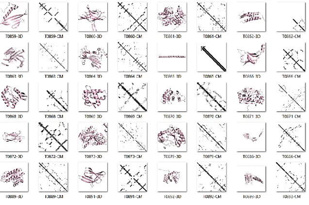
(35) For contact predictor evaluations it is more interesting to assess performance in FM targets, because in the absence of templates, contacts can provide us with constraints to explore the conformational space (Schaarschmidt et al., 2017). FM targets in the CASP12 dataset have low similarity. We try to use FastaHerder2 (Mier & Andrade-Navarro, 2016) to cluster sequences by similarity and size but it was not possible to obtain clusters because there are vast differences for all instances in the dataset. The full dataset has high variability in sequence length (standard deviation: 78.73 amino acids), with a minimum and maximum sequence size of 66 and 356 amino acids, respectively. In Figures 4 and 5 we show 3D structures for targets in CASP12. For each target, we show the cartoon representation and its CM. We notice that there are many differences between targets, which allow us to say that, as benchmark dataset, CASP12 targets are illustrative for the main protein families defined in SCOP (Andreeva et al., 2008). For top L/5, L/2 and FL contacts, the minimum for precision belongs to target T0863 which is the largest protein in the dataset and an all-α protein. This target was hard to predict because it has many α-helix/α-helix contacts at long sequence separation. RaptorX-Contact (S. Wang et al., 2018) and MetaPSICOV (Buchan & Jones, 2018) were the best predictors that succeeded predicting a few of these contacts (recall for secondary structure contacts (recall_ss) 13.15% and 10.810%, respectively). The protein with best predictions was the α+β target T0886, that has a more elongated structure. The average for FL precision, recall and recall_ss were 13.36%, 67.9%, and 83.2%. Recall and recall_ss indicate us that almost every. 22.

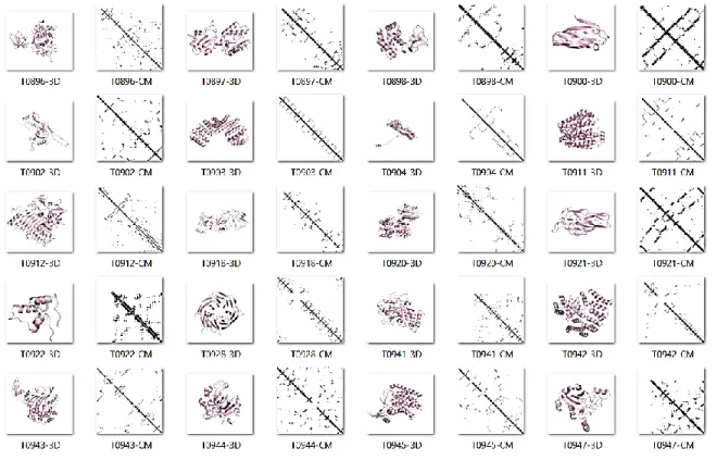
(36) predictor was able to predict many contacts in the protein, though the low precision is the result of many FP. For the top L/5 and L/2 contacts, the precision is greater because the list of predictions only includes some of the contacts that are more likely to be real contacts.. Figure 4. CASP12 PCP targets. First half. For each target, we display the 3D structure with a cartoon representation followed by its contact map.. 2.4. Top Predictors in CASP12 We used prediction results from the official CASP12 results web page. (predictioncenter.org/casp12/rrc_avrg_per_target_results.cgi, visited: November 2018) to select the top 10 predictors. From this top 10 we tried to identify the best predictors that would be an appropriate base for our novel predictor. The ranking. 23.

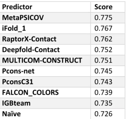
(37) score we applied was the average of F1, precision, recall, ES, ES_ext, MCC, recall_SS, MCC_SS y AUC_PR. To calculate the score, we scaled every measure by dividing it by its maximum value. Finally, the average was penalized by the proportion of targets submitted for the competition (for full submissions there is no penalization). In Table 2 we show the top 10 predictors ranked by our score.. Figure 5. CASP12 PCP targets. Second half. For each target, we display the 3D structure with a cartoon representation followed by its contact map. MetaPSICOV MetaPSICOV (Jones, Singh, Kosciolek, & Tetchner, 2015) combines predictions from three coevolution methods: PSICOV (Jones et al., 2012), mfDCA (Kaján et al., 2014) and CCMpred (Seemayer et al., 2014). MetaPSICOV performed as one of the top predictors by precision in RL top L/5 in CASP11 (Monastyrskyy et al.,. 24.

(38) 2015). In MetaPSICOV2 the pipeline uses MSAs from the reference databases PDB70, Uniref20, and Uniref100. The first step is to obtain alignments for the protein sequence against PDB70 using HHblits where subsequences with similarity greater than 98% are treated as template-based prediction and subsequences with lower similarity are handled as single domains. In the second step, MetaPSICOV2 tries to build a new alignment against Uniref20, and if the number of hits is below 2.000, a new alignment using JackHMER against Uniref100 is realized, followed of a new run of HHblits on this last result. The following steps are the same as for the previous version: local and global sequence features, coevolution scores, MI scores, and contact potential for columns i and j in the alignment. Table 2. Top 10 predictors CASP12 by an average of performance measures. The scores were reported in CASP12 website. Predictor MetaPSICOV iFold_1 RaptorX-Contact Deepfold-Contact MULTICOM-CONSTRUCT Pcons-net PconsC31 FALCON_COLORS IGBteam Naïve. Score 0.775 0.767 0.762 0.752 0.751 0.745 0.743 0.739 0.735 0.726. Local sequence features are calculated in three windows centered at positions i, j and (i+j)/2 and include amino acid composition in each window position; secondary structure probabilities; and solvent accessibility. Coevolution scores are. 25.

(39) obtained from PSICOV, mfDCA, and CCMpred. Two MI (Mutual Information) scores are used as defined in (Dunn et al., 2008). An averaged contact potential for columns i and j in the alignment is also incorporated. The last local features are associated with sequence separation for amino acids i, j at several ranges of separation. Global sequence features are calculated for the whole sequence and MSAs, including amino acid composition, secondary structure composition, average solvent accessibility, sequence length score, alignment size score, score for number of effective sequences in the MSAs, global average Shannon entropy. A set of 624 sequences extracted from the PDB with length in the range [50, 500] residues was used as input for training prediction models. Sequences were selected with identity lower than 25%, resolution at 1.5 Å and proteins that had similarity with proteins in PSICOV dataset (Jones et al., 2012) were identified and removed. The PSICOV dataset (150 proteins) and an additional dataset of 434 proteins with resolution at 2.0 Å and sequence length in the range [50, 400] residues were used for testing. In both, training and test datasets, overlapping sequences were excluded using HHsearch (Söding, 2005). MetaPSICOV uses the training dataset to build a new training dataset with the big set of features described above. This dataset of features (672 features × 634 proteins) is the input for the first stage of contact prediction. The training of the prediction model for this stage is realized using an architecture based on a feedforward neural network (two hidden layers), using for testing a subset of 10% of the initial training set.. 26.

(40) The contact map obtained by the first stage of training is reprocessed in the second stage by extracting an 11 × 11 window centered at positions i, j. The set of features described for the first stage is recalculated removing the window centered at position (i+j)/2 and expanding the windows around positions i and j. This new dataset of features (731 features × 634 proteins) is treated in the same way as in the first stage creating a new prediction model. DeepFold_ Contact, iFold_1, and naive The DeepContact Framework (Liu, Palmedo, Ye, Berger, & Peng, 2018) provides the architecture that is used for three predictors in the top 10 in Table 2: iFold_1, DeepFold_Contact and naive. The feature set used by DeepContact is similar to the one used by MetaPSICOV. The differences are that local features are calculated pairwise instead of windows around amino acids i and j and that there is no global score for sequence length. The features are used to create a training dataset from a subset extracted from the ASTRAL reference database (Chandonia, 2004) filtered at 40% of sequence identity. iFold_1, DeepFold_Contact and naive follow the prediction pipeline specified by DeepContact, but there are some differences in parameters and datasets. For training, DeepContact splits the training dataset into three bins: 80% for the training of prediction models, 10% for testing, and 10% for validation. To ensure data independence, all the sequences that belong to a superfamily are assigned to the same bin. Therefore, sequences in different bins can share only class and fold. The architecture used for training the prediction models implements convolutional 27.

(41) neural networks (CNN). CCN are widely used for image processing, speech recognition, drug design and genetic code analysis (Lecun, Bengio, & Hinton, 2015). In DeepContact, CNN are used in a two-fold way: Processing contact maps converted to images (2D features) and extracting statistical information related to amino acids (1D features). Deepfold_Contact implements an extra step that identifies domains and obtains MSAs using HHblits and JackHMMER. Naive does not identify domains and trains the prediction model on a separate dataset. iFold_1 generates a first MSA by means of HHBlits and if the MSA’s size if less than 1,000 sequences, it generates a larger alignment using JackHHMer. RaptorX-Contact RaptorX-Contact (S. Wang et al., 2018) is another predictor in our top 10 (Table 2), it is one of the first predictors to depend on deep learning for training PCP models, and it was already ranked in the top 10 in CASP11 (Monastyrskyy et al., 2015), just as MetaPSICOV. RaptorX-Contact implements an architecture similar to the one defined by DeepContact: one CNN for 1D features and another one for 2D features. The main feature in the design of RaptorX-Contact is considering the contacts as part of a whole (contact map) that are related to each other in contrast to many predictors that perform predictions for each possible amino acid pair in the protein sequence as if they were not part of a bigger structure.. 28.

(42) RaptorX-Contact was trained on a PDB25 subset that is obtained by removing any sequence with E-value < 0.1 when compared with the testing dataset. The testing data set included 150 Pfam families, CASP11 proteins, CAMEO proteins and a dataset of nonredundant membrane proteins. The training dataset size was 6300 proteins, and more than 400 proteins were used for testing. The first step of the training process converts 1D sequence features to a 2D representation. This 2D representation is used as input for a CNN which is fed to the 2D CNN. Finally, the previous 2D CNN includes as input 2D predictions for MI and a contact potential derived from CCMpred. For training, the dataset is divided into small bins of proteins of similar size and a few iterations are performed on each bin. The output of the last CNN is the probability for each residue pair to be in contact. During prediction, RaptorX-Contact generates four MSAs for each target using the reference database Uniprot20 (versions November-2015 and February2016) and E-values 0.001 and 1. The four predictions (one for each MSA) are averaged to obtain the final prediction. The in-house predictor RaptorX-Property (S. Wang, Li, Liu, & Xu, 2016) predicts local sequence features (secondary-structure, solvent accessibility, and disorder regions) and tries to model interrelationships between adjacent properties and sequence-structure. MULTICOM-CONSTRUCT The fifth predictor in our top 10, MULTICOM-CONSTRUCT, is part of a family of predictors that includes MULTICOM-NOVEL and MULTICOM-CLUSTER (Adhikari, Hou, & Cheng, 2018). MULTICOM-NOVEL integrates DNCON contact 29.

(43) predictions (Eickholt & Cheng, 2013) as the core of its pipelines. DNCON implements several sets of deep belief networks (DBN) that train models for several sequence window sizes in the range [7, 19] of residues. DNCON assembles the trained DBN using boosting and the set of features includes only sequence related and local features and excludes correlated mutations information. As in other approaches, DNCON centers windows on residues i and j and computes features such as secondary structure, sequence profile, solvent accessibility and a set of less common features derived from the statistical characterization of residues proposed by Atchley et al. (Atchley, Zhao, Fernandes, & Druke, 2005). For prediction, MULTICOM-CONSTRUCT generates MSAs using HHblits (reference database Uniprot20) and JackHMMER (reference database Uniref90) iteratively by relaxing parameters until the alignment reaches 2.5L sequences. MULTICOM-CONSTRUCT uses these MSAs as input for CCMpred, PSICOV, and FreeContact and then combines the predictions in the same way as for MetaPSICOV. PConsC31 and PCons-net PConsC31 and PCons-net are the next two predictors in our top 10 (Table 2). They are implemented based on PConsC2 (Skwark, Raimondi, Michel, & Elofsson, 2014) and PConsC3 (Skwark, Michel, Menéndez Hurtado, Ekeberg, & Elofsson, 2016).. 30.

(44) PConsC2 performs sixteen predictions for each input sequence, eight predictions using PSICOV and eight predictions using plmDCA, based on eight MSAs generated by HHblits and JackHMMER. The sixteen DCA predictions are integrated using the concept of neighborhood and that the contacts or non-contacts depend on the frequency of contacts/non-contacts in a 2D window with sizes in the range from 3 × 3 up to 11 × 11. PConsC2 trains prediction models using a deep learning approach of three layers of random forest with one hundred trees and integrates secondary structure prediction, solvent accessibility and sequence profiles using the PSICOV dataset. PConsC3 uses for training the PSICOV dataset extended with 30 small families. The testing dataset was the same of PConsC2. PConsC3 uses HHblits on Uniprot20 to generates MSAs for DCA using plmDCA and GaussDCA (Baldassi et al., 2014). For local and sequence related features PConsC3 relies on PhyCMAP (Z. Wang & Xu, 2013) that uses MI to estimate the contact probability of an amino acid pair and includes secondary structure and a distance statistical potential. PhyCMAP implements a prediction model supported on random forest and integer linear programming, which is less sensitive to the size of the MSAs. PConsC3 also integrates solvent accessibility and secondary structure using an algorithm analogous to CNN but replacing neural nets by random forest. The individual contact pair predictions are consolidated in a 2D 11 × 11 window. PConsC31 is the same as PConsC3 but using the best MSA generated by PConsC2.. 31.

(45) PCons-net is a combination that takes PConsC3 predictions as input for PConsFold, a pipeline for 3D structure prediction that uses the Rosetta folding protocol (Leaver-Fay et al., 2011) which refines a protein structure from short fragments. FALCON_COLORS FALCON_COLORS (Zhang et al., 2016) is the eighth predictor in our CASP12 top 10. FALCON_COLORS main difference is that it implements a special method (low-rank and sparse decomposition) to remove indirect coupling from correlation matrices obtained by using MI and mfDCA. FALCON_COLORS estimates parameters for low-rank and sparse decomposition using the PSICOV dataset. IGBTeam IGBTeam (Magnan & Baldi, 2014) is our ninth predictor and is another example of the success of deep learning, combining DCA information (CCMpred and FreeContact), in PCP. IGBTeam complements DCA with two in-house predictors for solvent accessibility (ACCpro) and secondary structure (SSpro). Considering the top 10 predictors described above, we want to emphasize the role of CCMpred and FreeContact for DCA prediction, the use of HHblits and JackHMMER for MSAs, the deep learning related approaches for training models used by every predictor in our CASP12 top 10 except FALCON_COLORS, and finally the importance of secondary structure and solvent accessibility which are used in. 32.

(46) almost every predictor. In Chapter IV, section 2.2, we analyze the performance of the ten predictors.. 3. Cellular Automata and PCP. A cellular automaton (CA) (Bhattacharjee, Naskar, Roy, & Das, 2018) provides us with a way to represent discrete dynamical models that allows depicting interconnections that affect the state of a system. The discrete space of a CA can be a matrix of finite integer values (states), and the interconnections of the system that it implements are expressed in terms of a window around each cell (neighborhood) in the matrix. CAs were devised by John von Newmann in the 1950s and have been since then widely studied and used in several knowledge domains. Wolfram (Wolfram, 2002) developed an extensive study on CAs dynamics for the simplest kind of CA: a matrix of 1 row × N columns; two states; neighborhood of radius 1 (size 3). Wolfram’s findings are well known, especially his behavior classification for dynamics in CAs. Bioinformatics and protein related phenomena have several successful cases in which CAs have been used to model dynamic behavior. A full recount of several applications related to genomics and proteomics was made by Chaudhuri et al. in a book that intends to summarize the application of CA models for biomolecules (Chaudhuri, Ghosh, Dutta, & Choudhury, 2018). Although there are no known applications of CA models in PCP, there are some interesting CAs that are used in proteomics. In (Chopra & Bender, 2007) Chopra and Bender designed a CA to. 33.

(47) predict secondary structure, using a genetic algorithm (GA). The GA was employed in the design of the CA because the rule that governs the secondary structure classification for a residue requires deep knowledge about how the values of the cell in a window of the sequence determine the secondary structure of each cell. The CA used by Chopra and Bender has a window of radius 5 (size 11) in a matrix of 1 row × L columns and three states (i.e., helix, beta sheet, and coil). The initial state for the matrix is assigned by DSSP (Kabsch & Sander, 1983) and propensities derived from Chou-Fasman parameters (P. Y. Chou & Fasman, 1974). The GA optimizes the weight associated with each neighbor in the window. In contrast to any other classification model, a CA achieves the final prediction after a successive application of the rule for several iterations, which allows the emergence of global implicit coordination and transference of information for the whole matrix. Chaudhuri et al. describe in (Chaudhuri, Parimal Pal Soumyabrata, Dutta, & Choudhury, 2018) a CA for modeling protein chains which uses a binary matrix of size 1 row × 8L columns. Each amino acid is represented by eight cells. For the CA representation of a protein, a set of sixty-four rules can be applied, and several features can be extracted from the evolution (iterative application of a rule) of the CA. The protein representation and the set of rules comprise a framework for analysis and experimentation of sequence manipulation. The analysis of binary patterns that emerge in the CA evolution allows obtaining measures for homogeneity, correlation, contrast, and entropy. The details of the CAs used by Chaudhuri et al. are described in (Ghosh, Maiti, & Chaudhuri, 2014).. 34.

(48) Neural-CA (Varela & Santos, 2018) is a very interesting approach that merges CAs and neural networks. Varela and Santos use a matrix 2D where each amino acid occupies the center of the edges in a unit cubic so that every amino acid has twelve neighbors. The neural-CA defines its states according to the hydrophobic polar (HP) model and uses evolutionary algorithms to optimize the neural-CA parameters. The neural-CA rule considers the energy landscape instead of the local spatial relationships in traditional CAs. The main aim of this approach is to create a framework for protein folding. However, the published tests only train models for specific targets, and their generalization capability is undetermined. Diao et al. describe an approach to predict the topology of transmembrane proteins in (Diao et al., 2008). This approach combines protein pseudo amino acid composition (K. C. Chou, 2011) with CAs. The representation of amino acids uses a binary chain of five bits and the CA’s matrix size is 1 row × 5L columns. This approach predicts the segment class in three categories (α-helix, β-strand, and non-trans membrane). The prediction process involves evolving the CA for twenty-six iterations to obtain a matrix of 26 rows × 5L columns (1 initial row plus 25 evolved rows). Lempel-Ziv complexity and pseudo amino acid composition are used to characterize the class for each segment. We hypothesize that CAs are able to evolve PCP from predictors such as CCMpred, FreeContact, and MetaPSICOV obtaining predictions with a less FP proportion. The idea is that a contact map is analogous to a 2D lattice of a CA with binary states and that we can learn the window (neighborhood) that defines. 35.

(49) interaction for contacts in the contact map and that the CA rule can evolve an initial contact map, predicted for CCMpred or any other predictor, towards a more nativelike contact map. To identify the CA’s neighborhood and rule, we have developed previously a GA (Díaz & Tischer, 2016) which we tested identifying a CA to reproduce a contact map folding trajectory from protein 2f4k. In Figure 6 we present a high-level representation of the pipeline for training and PCP based on CAs.. 4. Conclusions. We examined CASP12 results and selected a top 10 of predictors that were reviewed. The set of predictors that we selected represents the state of the art in PCP; we observe that every predictor in Table 2 shares these characteristics: 1. MSAs are generated using HHblits and JackHMMER adjusting parameters and selecting reference databases to optimize results. 2. Correlated mutations are fundamental for every predictor, though are used in diverse ways in each prediction pipeline. CCMpred and FreeContact are the main tools that predictors use to obtain MI or coevolution predictions. 3. Secondary structure, solvent accessibility, and sequence profiles provide complementary information to enhance PCP. 4. Sequence windows or contact map 2D windows allow predictors to consolidate profiles of features and to integrate patterns associated with contact identification.. 36.

(50) 5. Machine learning is the core for PCP models training. Deep learning and neural nets are the most popular approaches that predictors use in their training process.. Figure 6. Proposed pipeline for PCP training and CA-based PCP prediction. Structure modeling can be improved by using contact predictions. However, the current results require to improve the fraction of FP to allow modelers to enrich their result with information about real contacts.. 5. References. Adhikari, B., Hou, J., & Cheng, J. (2018). Protein contact prediction by integrating deep multiple sequence alignments, coevolution and machine learning. Proteins: Structure, Function and Bioinformatics, 86(June 2017), 84–96. https://doi.org/10.1002/prot.25405. 37.

(51) Adhikari, B., Nowotny, J., Bhattacharya, D., Hou, J., & Cheng, J. (2016). ConEVA: a toolbox for comprehensive assessment of protein contacts. BMC Bioinformatics, 17(1), 517. https://doi.org/10.1186/s12859-016-1404-z Altschul, S., Thomas, M., Alejandro, S., Zhang, J., Zhang, Z., Miller, W., & Lipman, D. (1997). Gapped BLAST and PSI-BLAST: a new generation of protein database search programs. Nucleic Acids Research, 25(17), 3389–3402. Andreeva, A., Howorth, D., Chandonia, J. M., Brenner, S. E., Hubbard, T. J. P., Chothia, C., & Murzin, A. G. (2008). Data growth and its impact on the SCOP database: New developments. Nucleic Acids Research, 36(SUPPL. 1), 419–425. https://doi.org/10.1093/nar/gkm993 Atchley, W. R., Zhao, J., Fernandes, A. D., & Druke, T. (2005). Solving the protein sequence metric problem. Proceedings of the National Academy of Sciences, 102(18), 6395–6400. https://doi.org/10.1073/pnas.0408677102 Baldassi, C., Zamparo, M., Feinauer, C., Procaccini, A., Zecchina, R., Weigt, M., & Pagnani, A. (2014). Fast and accurate multivariate Gaussian modeling of protein families: Predicting residue contacts and protein-interaction partners. PLoS ONE, 9(3), 1–12. https://doi.org/10.1371/journal.pone.0092721 Bateman, A., Martin, M. J., O’Donovan, C., Magrane, M., Alpi, E., Antunes, R., … Zhang, J. (2017). UniProt: The universal protein knowledgebase. Nucleic Acids Research, 45(D1), D158–D169. https://doi.org/10.1093/nar/gkw1099 Bhattacharjee, K., Naskar, N., Roy, S., & Das, S. (2018). A survey of cellular automata: types, dynamics, non-uniformity and applications. Natural Computing, 8, 1–29. https://doi.org/10.1007/s11047-018-9696-8 Buchan, D. W. A., & Jones, D. T. (2018). Improved protein contact predictions with the MetaPSICOV2 server in CASP12. Proteins: Structure, Function and Bioinformatics. https://doi.org/10.1002/prot.25379 Chandonia, J.-M. (2004). The ASTRAL Compendium in 2004. Nucleic Acids Research, 32(90001), 189D–192. https://doi.org/10.1093/nar/gkh034 Chaudhuri, Parimal Pal Soumyabrata, G., Dutta, A., & Choudhury, S. P. (2018). Cellular Automata (CA) Model for Protein. In A New Kind of Computational Biology (pp. 291–325). Singapore: Springer. Chaudhuri, P. P., Ghosh, S., Dutta, A., & Choudhury, S. P. (2018). A New Kind of Computational Biology. Singapore: Springer. https://doi.org/10.1007/978981-13-1639-5. 38.

(52) Chopra, P., & Bender, A. B. T.-I. S. B. (2007). Evolved cellular automata for protein secondary structure prediction imitate the determinants for folding observed in nature. In Silico Biology, 7(1), 87–93. Chou, K. C. (2011). Some remarks on protein attribute prediction and pseudo amino acid composition. Journal of Theoretical Biology, 273(1), 236–247. https://doi.org/10.1016/j.jtbi.2010.12.024 Chou, P. Y., & Fasman, G. D. (1974). Prediction of Protein Conformation. Biochemistry, 13(2), 222–245. https://doi.org/10.1021/bi00699a002 Demšar, J. (2006). Statistical comparisons of classifiers over multiple data sets. Journal of Machine Learning Research, 7(1), 1–30. https://doi.org/10.1016/j.jecp.2010.03.005 Diao, Y., Ma, D., Wen, Z., Yin, J., Xiang, J., & Li, M. B. T.-A. A. (2008). Using pseudo amino acid composition to predict transmembrane regions in protein: cellular automata and Lempel-Ziv complexity. Amino Acids, 34(1), 111–117. https://doi.org/10.1007/s00726-007-0550-z Díaz, N., & Tischer, I. (2016). Generic framework for mining cellular automata models on protein-folding simulations. Genetics and Molecular Research, 15(2), 1–16. https://doi.org/10.4238/gmr.15028654 Dunn, S. D., Wahl, L. M., & Gloor, G. B. (2008). Mutual information without the influence of phylogeny or entropy dramatically improves residue contact prediction. Bioinformatics, 24(3), 333–340. https://doi.org/10.1093/bioinformatics/btm604 Eickholt, J., & Cheng, J. (2013). A study and benchmark of DNcon: a method for protein residue-residue contact prediction using deep networks. BMC Bioinformatics, 14(Suppl 14), 1–8. https://doi.org/10.1186/1471-2105-14-S14-S12 Ekeberg, M., Lövkvist, C., Lan, Y., Weigt, M., & Aurell, E. (2013). Improved contact prediction in proteins: using pseudolikelihoods to infer Potts models. Physical Review E, 87(1), 1–19. Retrieved from http://pre.aps.org/abstract/PRE/v87/i1/e012707 Ghosh, S., Maiti, N. S., & Chaudhuri, P. P. (2014). Cellular automata model for protein structure synthesis (PSS). Lecture Notes in Computer Science (Including Subseries Lecture Notes in Artificial Intelligence and Lecture Notes in Bioinformatics), 8751, 268–277. https://doi.org/10.1007/978-3-31911520-7_28. 39.