Analysis of the influence of different variables on the impacts related with the envelope of buildings for residential use, with estimation of the interaction of the user

Texto completo

(1)Analysis of the influence of different variables on the impacts related with the envelope of buildings for residential use, with estimation of the interaction of the user.. Huedo Dorda, Patricia1, López-Mesa Belinda2, Mulet Elena1 1. Departamento de Ingeniería Mecánica y Construcción Universitat Jaume I, Castellón de la Plana, Spain 2. Universidad de Zaragoza, Spain. ABSTRACT There is an important mismatch, or gap, between the predicted and actual measurements of the impacts that are produced during the life cycle of buildings. This work aims to establish which variables exert a greater or lesser influence on the environmental impacts throughout the life cycle of the building and the weight of the user in the variation in heating consumption from. 1.

(2) information found in the literature and from data on real measurements of heating consumption in buildings.. The results show that, without taking the user into consideration, the climatic zone is the variable with the greatest influence, since it accounts for over 80% of the variation in heating consumption in the use phase. However, on analysing the influence of the user in zones with a continental climate, the results varied with respect to the predicted value from 5% in the case of low energy users up to more than 53% when they are high energy users. This means that the weight of high energy users in heating consumption is 35% and the relative weight of the climatic zone predicted by the regression model obtained with the energy simulation programs is reduced from 80% to 54%.. Key words: construction; environmental impact; LCA; gap; envelope.. 1. Introduction Policymakers are aware that one of the main ways of reducing energy consumption is to increase energy efficiency in the building sector (Allouhi et al., 2015). Designers find themselves before the increasingly more pressing obligation to provide data on the environmental impacts deriving from buildings and to justify with greater precision the use of building materials and solutions with a low environmental impact. The designer has to overcome the difficulty of combining two different but closely-linked scenarios: he/she needs to know to what extent the materials or the construction solutions used for the building are respectful to the environment and at the same time to what extent they are capable of guaranteeing a reduction in the energy. 2.

(3) demand, while maintaining the conditions of comfort of the building throughout the life thereof (Huedo et al., 2015). In the literature there are a number of studies based on Life Cycle Analysis (LCA) that have yielded accurate data on the weight of the impacts of each of the phases within the life cycle of a building, taking into account the envelopes and the emissions and consumptions of the HVAC installations (Gonzalo et al., 2000; Mithraratne and Vale, 2004; Alías and Jacobo, 2008; Gustavsson and Joelsson, 2009; Zabalza et al., 2009; Verbeeck and Hens, 2009; Ortiz et al., 2009; Ruá et al., 2010; Alonso et al., 2010; Estress Consultores, 2010; Wadel et al., 2011; IyerRaniga and Wong, 2012; Villar-Burke et al., 2014). Nevertheless, given the number of variables that come to bear on this relation and the widely varying results offered by these studies, more data are needed to develop models that make it possible to establish this link with greater precision. Although LCA is a rigorous method that studies the environmental impacts throughout the whole cycle, there is an important gap, or mismatch, between the predicted and actual measurements of the impacts that occur. The inaccuracy of the predictions in the different phases of the life cycle may be due to different factors that have been analysed in the literature (Norford et al., 1994; De Wit, 1995; Macdonald et al., 1999; UNE-EN 832/2000; Haas and Biermayr, 2000; De Wit, 2001; Menezes et al., 2011; Sendra Salas et al., 2013; López-Mesa et al., 2013a, 2013b; Wilde, 2014; Burmn et al., 2014; Nan Li et al., 2015; Blázquez et al., 2015, Xexakis and Dobbelsteen, 2015; Herrando et al., 2016;. Dronkelaar et al., 2016. This gap not only. affects new building projects, but also occurs in the predictions that are made regarding existing buildings before and after being refurbished, in which neither the expectations concerning energy savings nor the term calculated to amortise the investment are met López-Mesa et al., 2013a.. 3.

(4) On the one hand, the gap may be due to causes that can be attributed to the actual prediction methodology employed, since LCA studies on buildings have often had to simplify the method used and also carry out adaptations and approximations when it comes to working with the data available in the sources of information (Ecoinvent, Buwal 250, Idema, Ivam etc.) KTH et al., 2010). Moreover, the environmental impact inventories in the LCA require a high level of information about materials and processes, which may not be available for a wide range of situations. Likewise, it is difficult to calibrate the environmental impacts produced during the use phase because there are many variables involved in this stage that are not always taken into consideration by simulation software (EnergyPlus, Ecotect, eQues, Lider, Calener, etc.), and basically affect the conditions of usage of each (Huedo, 2014). Nan Li et al. attribute this discrepancy to the occupancy data or to the conditions of the building chosen as a reference (Nan Li, 2025). Hence, after analysing the causes of the gap they focused on developing systems with which to achieve a better calibration of the reference model. Other authors such as Blazquez et al. (2015) consider that the divergences between actual and simulated results are due to uncertainty and the lack of information about the usage and operating conditions. Likewise, Xexakis and Dobbelsteen claim that the performance of a building is affected by a large number of interconnected para meters that vary according to the type, construction, location and, above all, the user's way of life, which is one of the most unpredictable variables (Xexakis and Dobbelsteen, 2015). In this same line, several studies such as Wilde (2014) and Hernado et al.,(2016) claim that the average difference between the predicted and the actual consumption of residential buildings stands at around 30%, and also analyses a number of different factors that can be responsible for this mismatch. Wilde places special emphasis on the impact of the outdoor climate and concludes that the maximum variation. 4.

(5) occurs in the presence of extreme outdoor temperatures, whereas the gap is considerably lower if the outside temperature is between 16oC and 18oC, which is when it is not necessary to use heating or air conditioning (Wilde, 2014). Lopez-Mesa et al. measured the energy behaviour of some dwellings in a block of apartments on the Girón residential estate in Zaragoza before and after being refurbished and compared the data obtained by means of simulation software with the real measurement of the consumptions. This study revealed that after refurbishment the expected energy savings did not occur. Thus, they concluded that this mismatch in the predictions was due to two remarkable suppositions: in some cases, the energy consumption increased by far less than was expected due to the fact that the energy habits of the owners varied following the refurbishment, thereby allowing them to gain increased thermal comfort in their homes. In other cases, the researchers found that the conditions of use varied depending on the socio-economic level of the user, observing that users often did without an adequate level of thermal comfort so as to match their energy consumption to their purchasing power. In some social sectors financial savings prevailed over comfortable living conditions in situations of true “energy poverty” (Lopez-Mesa et al., 2013b). From all the above it is obvious that to be able to determine the energy and environmental behaviour of our buildings it would be essential to monitor them under real living conditions. But even so, measuring real data for a building does not imply that the same results are to be found in other similar buildings. Nevertheless, the designer must be able to ensure, in the initial stages of the design, the environmental requirements of the Regulations are complied with by maintaining the required level of comfort, when real measurements are still not available.. 5.

(6) As we understand it, in order to aid the designer, it would be useful to know which variables can exert a greater or lesser influence on the production of environmental impacts throughout the life cycle of the building and to explore the extent to which the transversal interaction of the user with these variables could help to calibrate the gap between the prediction and the actual measurement of the impacts that are produced. Thus, in view of the difficulty involved in predicting the impacts and establishing the environmental benefits that require the selection of certain alternatives in the design in both new and refurbished buildings, this work considers it important to analyse those aspects that can affect the appraisal of the environmental impact of the building by exploring how the user's behaviour influences the outcome.. 2. Aims. The aim of this work is to use a multiple linear regression model to investigate which of the explanatory variables involved in the design phase can exert a greater or lesser influence on the production of environmental impacts throughout the life cycle of the building. It also seeks to estimate the weight of the users by considering them as a variable that modifies the predicted values and, therefore, the weight of the different variables. The specific aims are: -. To estimate the weight of the climatic zone, the orientation and the type of façade, roof and carpentry employed in the envelope in the impacts of the use phase.. -. To establish a preliminary estimation of the influence of the user's behaviour on the impact on the consumption of heating energy.. 6.

(7) -. To estimate the saving that can be achieved in water consumption and waste generation depending on the type of envelope that is chosen.. With these data the aim is to help reduce the gap between the predicted and real measurements of the impacts produced by selecting construction solutions with a low environmental impact that improve the conditions of comfort of the dwellings, both in new and in refurbished buildings, while calibrating the uncertainty due to user interaction.. 3. Description of the prediction model used. In previous studies a model for predicting the impacts caused by the envelope throughout its life cycle was obtained (Huedo et al., 2016a). This model was developed by applying a simplified LCA method for a single-family terraced house with 180 alternatives for the design of the envelope combined with two climatic zones and two orientations. In order to obtain the impacts of the manufacturing stage, the TCQ2000 tool was chosen, and more specifically its environmental management module TCQGMA, since it is a software application that is readily available due to the existence of agreements allowing it to be used by students and researchers at low cost. Moreover, this program has already been used by several different authors (Zabalza et al., 2009; Ortiz et al., 2009; Estress Consultores, 2010; Wadel et al., 2011; Iyer-Raniga and Wong, 2012; Villar-Burke et al., 2014). The impacts in the use phase were obtained by means of the energy simulation tools LIDER and CALENER, which made it possible to calculate the energy consumptions and CO2 emissions, as these tools ensure compliance with the requirements set out in the Documento. 7.

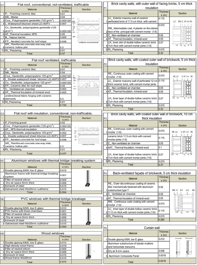
(8) Básico de Ahorro de Energía del Código Técnico de la Edificación en España (CTE, 2006) (Energy Saving Basic Document in the Spanish Technical Building Code. These same software tools were also used in some of the research studies mentioned above (Zabalza et al., 2009; Ortiz et al., 2009; Ruá et al., 2010). In developing this model, when it came to applying the LCA methodology, a set of standard methodologies published by Technical Committee 350 of the European Committee for Standardisation (CEN/TC 350) were taken into account. These are outlined below. The case study chosen for use in this model was a single-family terraced house that has two floors and an usable floor area of 93.5 m2 (Figures 1 and 2).. Figure 1. Section of the dwelling used as a case study. Figure 2. Plan views of the dwelling used as a case study. A functional unit of 1m2 of usable floor area and a useful lifespan of the building of 50 years were chosen. In this case the explanatory variables were taken as being each of the construction assemblies that make up the envelope (a type of roof C, a type of façade F and a type of carpentry H). Table 1 shows three assemblies that are most commonly employed for the building envelope and which were chosen for this study. Each construction assembly is designated with a capital letter that indicates the class (C = roof, F = façade and H = carpentry) and their numerical index that indicates the type of building assembly (Huedo et al., 2016b).. 8.

(9) C1. Flat roof, conventional, not-ventilated, trafficable Material. Thicknes s (m) 0.01 0.04. 1 P_ Finishing ceramic tiles 2 MA_ Mortar 2 3 Csa_ Polypropylene geotextile (125 gr/m ) 4 I_ Waterproof bitumen sheet LO-40/FV. 0.000128 0.007. Cs_Geotextile, polypropylene geotextile (125 2 5 gr/m ) 6 AT_Thermal insulation XPS 7 B_ Vapour barrier. 0.000128 0.05 0.005. 8 FP_ Aerated concrete for roof slope SR_ Reinforced concrete one-way slab, 9 ceramic hollow plot 10 RI_ Plastering Total C2. 0.048 0.3 0.01 0.47. 1 P_ Finishing ceramic tiles 2 MA_ Mortar 2 3 Csa_ Geotextile, polypropylene 125 gr/m 4 I_ Double waterproof sheet bitumen LO-40/FV 2 5 Cs_ Geotextile, polypropylene 125 gr/m 6 FP_ Ceramic tiles for roof slope 7 C_ Ventilated air chamber of mineral 8 AT__ Thermal Insulation pp y wool unidirectional fabric forging with ceramic 9 elements 10 RI_Plastering Total. Thicknes s (m) 0.01 0.04. 6 FP_ Aerated concrete for roof slope. 0.048. SR_ Reinforced concrete one-way slab, 7 ceramic hollow plot 8 RI_ Plastering Total. H2. Double glazing 6/6/6, low E glass PVC frame with three chambers Filler of neutral silicon Dry air space 6mm thick Ironwork of steel Galvanized steel 40x20mm subframe Total. 1 2 3 4 5 6. Material Double glazing 6/6/6, low E glass High density wood frame Filler of neutral silicon Dry air space 6mm thick Ironwork of steel Wood frame 40x20mm Total. 0.015. 0.05 0.05. Brick cavity walls, with coated outer wall of brickwork, 10 cm thick insulation Thicknes s (m). 0.3 0.01. 4 AAT_ Thermal Insulation, mineral wool. 0.1. 0.437. LH_ Inner layer of double hollow ceramic brick 0.07 5 7cm thick with cement mortar joints (1:6) 6 RI_ Plastering 0.015 Total 0.37. Section. 0.012. F4. 0.001. Thicknes s (m) 0.012 0.001 0.005 0.006 0.015 0.015 0.054. Thicknes s (m) 0.012 0.019 0.005 0.006 0.015 0.015 0.072. Thicknes s (m). RE_ Outer discontinuous coating of ceramic tiles mechanically fastened with aluminium 1 substructure type T 2 C_ Ventilated air chamber. Section. 3 AT_ Thermal Insulation of mineral wool RM_ Continuous outer coating with cement 4 mortar (1:6) LC_ Inner layer of double hollow ceramic brick 5 11.5 cm thick with cement mortar joints (1:6) 6 RI_ Plastering Total. Section. 0.02 0.05 0.05 0.015 0.115 0.015 0.265. Curtain wall. F5 Material Section. 0.115. Back-ventilated façade of brickwork, 5 cm thick insulation Material. 0.005 0.006 0.015 0.015 0.054. Section. 0.015. 0.05. Thicknes s (m). Section. 0.115. ceramic brick 11.5 cm thick with cement 2 mortar joints (1:6) 3 C_ Non-ventilated air chamber. Wood windows. H3. F3. Material RE_ Continuous outer coating with cement 1 mortar _ (1:6) y. 0.000128 0.05. PVC windows with thermal bridge breakage Material. 1 2 3 4 5 6. Section. Aluminium windows with thermal bridge breaking system Material Double glazing 6/6/6, low E glass Aluminium frame with thermal bridge breaking system Filler of neutral silicon Dry air space 6mm thick Ironwork of steel Galvanized steel 40x20mm subframe Total. Thicknes s (m). LH_ Inner layer of double hollow ceramic brick 0.07 5 7cm thick with cement mortar joints (1:6) 6 RI_ Plastering 0.015 Total 0.32. 0.3 0.01 0.725. Thicknes s (m) 0.02. Section. Brick cavity walls, with coated outer wall of brickwork, 5 cm thick insulation. RE_ Continuous outer coating with cement 1 mortar (1:6) LC_ Exterior masonry wall of perforated 12 cm 2 thick ceramic brick, with cement mortar joints 3 C_ Non-ventilated air chamber 4 AT_ Thermal Insulation, mineral wool. 0.000128 0.35 0.003 0.005. 0.002 0.007. 2 3 4 5 6. F2. Material. 0.000128 0.007. 1 P_Finishing gravel 2 2 Csa_ Polypropylene geotextile (125 gr/m ) 3 AT_ XPS thermal insulation 2 4 Csa_ Geotextile, polypropylene 125 gr/m 5 I_ Double waterproof sheet bitumen LO-40/FV. 1. Section. Brick cavity walls, with outer wall of facing bricks, 5 cm thick insulation. Thicknes Material s (m) LC_ Exterior masonry wall of ceramic 0.115 1 perforated brick of 11.5 cm thick, with cement 0.015 RM_ Intermediate coat. A plaster on the interior 2 face of the principal with cement mortar (1:6) 3 C_ Non-ventilated air chamber 0.05 0.05 4 AT_ Thermal Insulation, mineral wool LH_ Inner skin of double hollow ceramic brick 0.07 5 7cm thick with cement mortar joints (1:6) 6 RI_ Plastering 0.015 0.32 Total. Flat roof with insulation, conventional, non-trafficable. Material. H1. F1. Flat roof ventilated, trafficable Material. C3. Section. 1 Double glazing 6/8/6, low E glass. Thicknes s (m). Section. 0.012. Aluminium substructure of tubular mullions 2 and horizontals transoms 3 Dry air 8 mm space. 0.008. 5 Aluminium Composite Panel. 0.0018. Total. 0.0218. Table 1. Characterisation of the construction assemblies assessed. 9.

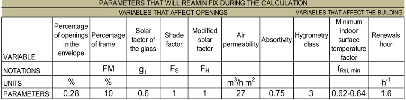
(10) The calculations were performed by combining, in each alternative, a type of roof, a type of façade and a type of carpentry, in a climatic zone and an orientation. For the purposes of this study, to be able to obtain comparable results, two climatic zones were selected: B3 and E1. Climatic zone B3 has a temperate and humid climate with a mean annual temperature of around 17.8°C, while climatic zone E1 has a cold dry climate, with a mean annual temperature of about 12.2°C. Likewise, the calculations were performed in two orientations: North-east (NE) and South-east (SE). Table 2 shows all the explanatory variables that were taken into consideration. Construction assemblies of the envelope Variable Roof system Façade system Notations. C1. C2 C3. F1. F2. F3. F4. F5. Carpentry system H1 H2 H3. Units. m2. m2. m2. m2. m2. m2. m2. m2. m2. Climatic zones B3 E1. Orientations NE. SE. m2. Table 2. Explanatory variables Altogether 45 combinations of construction assemblies were evaluated in two orientations and two climatic zones each, that is, a total of 180 options. The other parameters, as regards openings and with regard to the building, are taken as fixed, with the values shown in Table 3. PARAMETERS THAT WILL REAMIN FIX DURING THE CALCULATION VARIABLES THAT AFFECT OPENINGS. VARIABLE. Percentage Solar of openings Percentage factor of in the of frame the glass envelope. FM. NOTATIONS UNITS PARAMETERS. % 0.28. % 10. g. Shade factor. FS. VARIABLES THAT AFFECT THE BUILDING. Minimum Modified indoor Air Hygrometry Renewals solar Absortivity surface permeability class hour factor temperature factor. FH. f Rsi, min 3. 0.6. 1. 1. m /h m 27. 2. 0.75. 3. 0.62-0.64. h-1 1.6. Table 3. Parameters that were taken as fixed. 10.

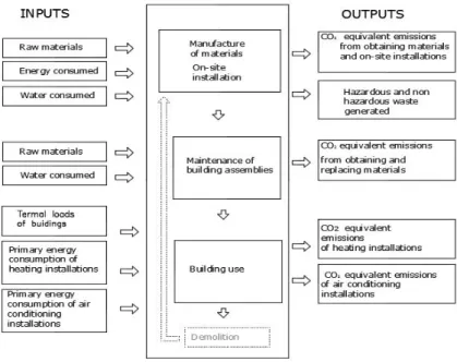
(11) In order to calculate the impacts, all the energy and material inlets and outlets were identified together with the emissions generated for each of the phases to be assessed, as can be seen in Figure 3.. Figure 3. Diagram of the inventory analysis. In the manufacturing and installation phase, the data concerning the constitutive materials (density, thickness, specific weight) were obtained from the CTE catalogue of construction assemblies and the environmental and costs data were obtained from the BEDEC (2013) database. The impact in the manufacturing phase was obtained using the TCQ2000 (2013) tool. The impact during the maintenance phase, on the other hand, was obtained by assigning a reconditioning factor, RF, to each of the constituent elements, depending on the number of times. 11.

(12) that material would have to be replaced throughout the lifespan of the building (Hernandez Moreno, 2011). The impact in the use phase was obtained by introducing the data on the 180 design options outlined earlier into LIDER (2011) and then calculating with CALENER (2011). The impacts evaluated by this model are:. - The global warming potential or greenhouse effect emissions shows the total greenhouse gas emissions in CO2 equivalent emissions per m2 of usable floor space in the building resulting from the production and transformation of the construction materials during the manufacturing and maintenance phase and the consumption of the installations during the use phase related to the construction solutions employed in the building envelope. Unit of measurement: CO2 equivalent emissions/m2. - The primary energy consumption per m2 of usable floor area of the building due to the production and transformation of construction materials during the manufacturing and maintenance phase, as well as the consumption of the installations in the building during the use phase related with the building solutions used in the building envelope. Unit of measurement: kWh/m2. - Water consumption is the amount of fresh water consumed per square metre of usable floor area of the building, taking into account all the water consumed in the manufacturing of materials and their on-site installation. Unit of measurement: m3/m2. - Waste generated in Kg/m2 of usable floor area of the building, taking into account the hazardous and non-hazardous waste generated in the manufacturing and installation phase, including packaging waste. Unit of measurement: Kg/m2. The results obtained in the use phase were taken to produce the following equations with which to predict the impact from the explanatory variables shown in Table 2.. 12.

(13) Thus, for example, bearing in mind that three types of roof have been considered, if the hot flat roof C1 is part of a construction solution, then the number 1 will appear in the corresponding box and box C2 will have a 0. The other construction assemblies are coded in the same way. ∈. ,. 23.6924 0.49 1. 18.06 3. 0.05. 0.07 2. 0.20 1. 2.31 4. 0.84 3. 2.28 2. 2.62 1 1. 0.67 2. ∈ 1.5787 2. 4.66 3. 116.4009 3.21 2. 0.01. 89.40 3 1.44 1. 0.03 2. 0.10. 6.2829 18.65 3 0.01 0.46 2 0.48 1. 0.08 1. 0.27 2. 0.23 2. 1.37 4. ∈ 1.27 1. 0.30 1. ∨ 1.49 3. 1.45 2. 12.73 4. ∈ 5.54 4. 1.44 1. 5.36 3. 6.02 3. 0.08 2. 12.93 2 3. 5.81 2. 0.09 1. 14.32 1. 5.78 1 4. 4. Methodology. The equations that predict the impact of the use phase according to the explanatory variables will be used to evaluate the relation between each of the explanatory variables under consideration and the dependent variables, which are the impacts under evaluation. The next step is to take into account the fact that, as pointed out in some studies, user intervention can act as a effect-modifying variable. Therefore, an analysis will be performed to detect the interaction of the user with the independent variables and with the impacts, based on the data collected from the literature. Finally, the results will be analysed. A diagram showing the methodology to be followed can be seen in Figure 4, where the work tasks described in this paper are highlighted in bold type.. 13.

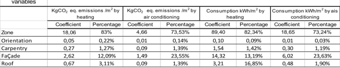
(14) 1st Phase: application of simplified LCA methodology. 3rd Phase: appraisal of results. 2nd Phase: Obtaining the multiple linear regression modelling. 1. Aim and scope 2. Analysis of inventory 3. Impact assessment 4. Interpretation of results. Study of the influence of each variable Analysis to detect the user interaction. Conclusions. Figure 4. Diagram of the application of the methodology The next section shows the results obtained.. 5. Results 5.1. Estimation of the weight of the climatic zone, the orientation and the solutions used in the envelope in the impacts of the use phase These equations allow us to determine the contribution of each of the variables in the process of obtaining the impact. Table 4 shows the resulting coefficients for each of the explanatory variables and the percentage that shows the extent of the influence which each of these variables exerts on the value of the impact. The value of the coefficients is the difference between the maximum and the minimum values of each of the coefficients of the explanatory variables.. Explanatory variables. Dependent variables = impacts produced during the use phase per m2 of usable surfase area of the dwelling KgCO2 eq. emissions /m 2 by heating. KgCO2 eq. emissions /m 2 by air conditioning. Coefficient. Consumption kWh/m 2 by heating. Consumption kWh/m 2 by ais conditioning. Coefficient. Percentage. Percentage. Coefficient. Percentage. Coefficient. Percentage. Zone. 18,06. 83%. 4,66. 73,53%. 89,40. 82,34%. 18,65. 73,24%. Orientation Carpentry FaÇade Roof. 0,05 0,27 2,62 0,67. 0,22% 1,27% 12,09% 3,11%. 0,01 0,09 1,49 0,09. 0,14% 1,39% 23,55% 1,39%. 0,10 1,54 14,32 3,21. 0,09% 1,42% 13,19% 16,85%. 0,01 0,30 6,02 0,48. 0,03% 1,19% 23,63% 1,90%. Table 4. Extent of the contribution made by each variable to the impacts of the use phase. 14.

(15) As can be seen, the variable that has most influence on the variation of the CO2 equivalent emissions is the climatic zone, and the weight of the zone is greater in heating (about 83%) than in air conditioning (about 73%). The variable with the second highest weight is the type of façade, which has more influence on the demand for air conditioning (23%) than for heating (12%). The other variables in the regression model have a much lower weight.. 5.2. Weight correction based on the estimation of the user effect. As pointed out in the introduction, the mean value of the gap is around 30% in buildings for residential use. Hence, one option to reduce the gap between the calculated data and the real behaviour of the building would be to correct the value of the results using data from the literature in order to obtain a range, and then adjust the weights in accordance with the following equation: IR = IE + 30% IE. [5]. where IR = Real Impact IE = Estimated Impact. In the introduction it was also stated that the gap between the actual and the calculated impacts is variable and largely depends on the climatic zone. Its maximum value is obtained in extreme outdoor temperatures and it is considerably lower if the outdoor temperature is between 16oC and 18oC (Wilde, 2014b).. 15.

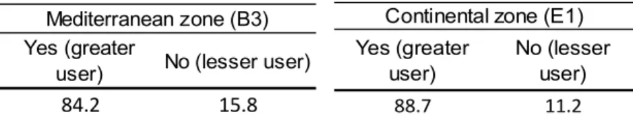
(16) Moreover, under certain circumstances, the variation between the real and the predicted consumption is only 5%, since the user with low purchasing power lives below the required conditions of comfort, in a state of “energy poverty” (López-Mesa et al.,2013a). In order to reduce the gap between the estimated impact and the actual value of the impact due to the energy consumption on heating an analysis was performed to determine the interaction of a new variable (effect-modifying variable), in this case the influence of the user (Iu) on the relationship between two variables: climatic zone and energy consumption. For this purpose, two strata of the explanatory variable “climatic zone” were considered (B3 and E1) depending on the outdoor temperature.. 1. First, the average monthly temperatures were obtained for each of the climatic zones, according to data published in the Guía técnica de Condiciones climáticas exteriores de Proyecto (Technical Guide to Outdoor Climatic Conditions of the Project) (IDAE, 2010).. Mediterranean zone (B3) January. 10.4. February. 11.0. March. 13.2. April. 16.1. May. 18.9. June. 23.2. July. 25.2. August. 25.7. September. 23.1. October. 19.7. November December. 14.1. 10.2. Continental zone (E1) January. 6.3. February. 6.7. March. 9.9. April. 13.5. May. 16.0. June. 21.1. July. 23.0. August. 23.4. September. 20.4. October. 16.3. November December. 9.8. 5.9. Table 5. Mean monthly temperature by climatic zones. 2. The next step was to establish the percentage of users with higher energy demands (“high energy users”) and those with lower energy demands (“low energy users”), depending on the number of homes that do not fulfil the conditions of comfort required in winter for each climatic zone, based on the results of surveys published by the INE (Spanish National Institute of Statistics) (INE, 2008) (Table 6).. 16.

(17) Mediterranean zone (B3) Yes (greater No (lesser user) user). 84.2. 15.8. Continental zone (E1) Yes (greater user). No (lesser user). 88.7. 11.2. Table 6. Percentage of high and low heating energy users by purchasing power As has already been said, previous studies reveal that users mainly switch on the heating when the outdoor temperature drops below 17°C. Thus, the data in Table 5 were used to calculate the percentage of days where there is a demand for heating and this was applied to the percentage of high and low energy users in Table 6, the result being the data shown in Table 7. This analysis has made it possible to obtain a range of percentage values (mu) that indicate the interaction of the user in each climatic zone depending on the outdoor temperature and the user's purchasing power.. User intervention. ZONE E1: Continental climate annual % user mu Total intervention by temperature percentage m u 0 outdoors < 17. % users (higher or lower energy users owing to their purchasing power). YES. NO. YES (greater user). 56,1. 32,6. 88,8. No (lesser user). 7,1. 4,1. 11,2. Total percentage m u. 63,2. 36,8. 100,0. ZONE B3: Mediterranean climate User intervention. annual % user mu Total intervention by temperature percentage m u 0 outdoors < 17. % users (higher or lower energy users owing to their purchasing power). SI. NO. YES (greater user). 43,8. 40,4. 84,2. No (lesser user). 8,2. 7,6. 15,8. Total percentage m u. 52,0. 48,0. 100,0. Table 7. Incidence factor (mu) of high and low energy users in each climatic zone according to the outdoor temperature. 17.

(18) These results can be explained by the interaction phenomenon, since the intensity of the relation between user and energy consumption is modified by the outdoor temperature and by the user's purchasing power. Once the incidence factor (mu) is known from the information in the statistical databases and from the climatological behaviour, we need to know how the consumption will vary with respect to that predicted by the model (Equation 3). The factors taken into consideration are: -. User intervention only takes place if the outside temperature is below 17°C.. -. Over a period of one year, a user intervention that was not predicted by the model will be taken into account, with values of 7.1% for the low energy users and 56.1% for the high energy users. -. The value of the intervention of the low energy (poorer) user Iund with respect to the estimated impact (IE) is Iund = 5% IE, obtained from the actual measurements published by Lopez-Mesa et al. (2013b).. -. The mean value of the gap between the actual and the predicted values is, without differentiating between types of user, 30%.. -. Thus, the value of the high energy (wealthier) user's intervention Iud has been calculated by comparing the mean value of the gap with the average of the intervention of the type of user, in accordance with the following equation:. 0.3 IE =. .. .. ,. [6]. 7.1 (0.05 IE) + 56.1 Iud = 30 IE. 18.

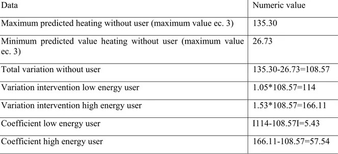
(19) Hence, the value of Iud that corresponds to a high energy (wealthier) user is Iud = 52.8% IE.. We know that the gap is produced between the values 0.05 , 0.528. , and therefore, by. substituting these values in Equation [5], we see that the real impact of heating consumption is equal to the expected impact from the model, adjusting it between those values, as indicated in Equation [7]. IR = IE + 0.05,0.53 IE. [7]. This equation allows us to adjust the real heating consumption depending on the estimated impact and on the interaction of the variable Iu (user intervention), the value of which can be chosen depending on the user's purchasing power.. 5.3. Estimation of the weight of the explanatory variables that take the user intervention into account in the heating consumption. Table 7 shows the weight of each of the explanatory variables used in the regression model without taking into account the intervention of the user. As the variation interval of the heating consumption according to the type of user behaviour has already been analysed in the previous section, the weights of all the explanatory variables have been recalculated, with the inclusion of the user. Table 8 shows the coefficients obtained for a low energy and a high energy user.. 19.

(20) Data. Numeric value. Maximum predicted heating without user (maximum value ec. 3). 135.30. Minimum predicted value heating without user (maximum value 26.73 ec. 3) Total variation without user. 135.30-26.73=108.57. Variation intervention low energy user. 1.05*108.57=114. Variation intervention high energy user. 1.53*108.57=166.11. Coefficient low energy user. I114-108.57I=5.43. Coefficient high energy user. 166.11-108.57=57.54. Table 8. Obtaining the coefficients of user intervention for heating consumption in the continental climate zone. Table 9 shows the influence of all the variables obtained in the regression model taking into account the influence of the user as an effect-modifying variable. Weight of the variables in heating consumption. Zone E1, continental climate Low energy user High energy user Explanatory Weight Explanatory variable Coefficient (%) variable Coefficient Weight (%) Zone 89.4 78.4% Zone 89.4 53.8% Orientation. 0.1. 0.1%. Orientation. 0.1. 0.1%. Carpentry. 1.54. 1.4%. Carpentry. 1.54. 0.9%. Façade. 14.32. 12.6%. Façade. 14.32. 8.6%. Roof. 3.21. 2.8%. Roof. 3.21. 1.9%. Low energy user. 5.43. 4.8%. High energy user. 57.54. 34.6%. Table 9. Degree of contribution of each variable to heating consumption in climatic zone E1. 20.

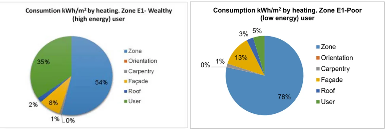
(21) As can be seen in Table 9, the weight of the high energy users in heating consumption is 35% and the relative weight of the climatic zone predicted by the regression model obtained from the energy simulation programs drops from 80% to 54%.. If the results in Table 9 are compared, it can be seen that the interaction of the user modifies the weight of the other variables; hence, if the user has a heavy demand for energy, the influence of the climatic zone changes from 78% to 54%. The influence of the envelope on the energy consumption of the building in the use phase has also been calculated, the result indicating that the weight of the envelope has twice as much effect when the user is a low energy consumer (Figure 5).. Consumption kWh/m2 by heating. Zone E1-Poor (low energy) user 3% 5% Zone 0%. 1%. 13%. Orientation Carpentry Façade 78%. Roof User. Figure 5. Weight of the explanatory variables in the impact due to the energy consumption by heating in the supposed case of intervention by a low energy and high energy user. Likewise, the results obtained have allowed us to determine the proportion represented by the impacts that occur at the beginning of the life cycle of the building due to the manufacturing and installation of the materials with respect to both the impacts produced during the maintenance. 21.

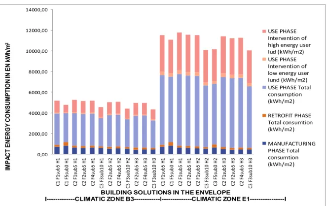
(22) phase as a result of refurbishment and the impacts produced mainly by the heating and air conditioning installations, taking into account the user interaction (Figure 5). It has been shown that during the use phase, the intervention of a high energy user can increase the estimated value of the impact by about 50%, the weight of the user being 35% of the total for the use phase. A low energy user, however, modifies the predicted impact by barely 5% (López-Mesa et al., 2013b).. 14000,00. USE PHASE Intervention of high energy user Iud (kWh/m2) USE PHASE Intervention of low energy user Iund (kWh/m2) USE PHASE Total consumption (kWh/m2). 10000,00. 8000,00. 6000,00. 4000,00. RETROFIT PHASE Total consumtion (kWh/m2). 2000,00. C2 F4sub5 H3. C3 F3sub10 H3. C2 F2sub5 H3. C2 F1sub5 H3. C3 F5sub0 H2. C2 F1sub5 H2. C3 F3sub10 H2. C2 F2sub5 H1. C2 F1sub5 H1. C1 F5sub0 H1. C1 F1sub5 H1. C2 F4sub5 H3. C3 F3sub10 H3. C2 F2sub5 H3. C2 F4sub5 H2. C3 F3sub10 H2. C2 F2sub5 H2. C2 F4sub5 H1. C3 F3sub10 H1. C2 F2sub5 H1. C2 F1sub5 H1. C1 F5sub0 H1. 0,00. C1 F1sub5 H1. IMPACT ENERGY CONSUMPTION IN EN kWh/m2. 12000,00. MANUFACTURING PHASE Total consumtion (kWh/m2). BUILDING SOLUTIONS IN THE ENVELOPE I-------------CLIMATIC ZONE B3------------I--------------CLIMATIC ZONE E1----------------I. Figure 6. Comparison of the impact due to the energy consumption on heating throughout the life cycle of the building, taking into consideration the interaction of the user in the use phase If we analyse the results obtained in zone E1, orientation NE, the difference between the primary energy consumptions deriving from the combination C1F5H1 (11222.00 kWh/m2) and those related to the combination C3F3H3 (9773.1 kWh/m2) over a period of 50 years, with a high. 22.

(23) energy user, is 1448.09 KWh/m2, that is to say, 12.90% less consumption of primary energy over 50 years, depending on the combination that is chosen (Figure 6). In this same climatic zone and orientation, the difference between the CO2 equivalent emissions related to C1F5H1 (2497.04 kg CO2eq.) and those related to combination C3F3H3 (2097.11 kg CO2eq.) is (399.93 kg CO2eq.), that is to say, 16.01% less CO2 equivalent emissions, depending on the combination that is chosen.. 5.4. Impact of the envelope on water consumption and waste generation It has also been observed that other impacts related with the envelope, such as water consumption and waste generation, occur mainly in the initial phases of the life cycle and have a lesser effect in the maintenance and use phases. These impacts basically depend on the building solutions evaluated and do not vary according to the climatic zone or the user. - With regard to water consumption, the difference between the solution that consumes the least water, C2F5H1 (0.01 m3), and the solutions that consume the most water, C1F1H1 or C3F1H1 (0.05m3), is 0.04 m3 of water per m2 of usable floor area, which amounts to 80% less water. In general more water is consumed by combinations that use concrete or mortar in the implementation phase, whereas less water is consumed by the combinations that make use of prefabricated solutions (Figure 7).. 23.

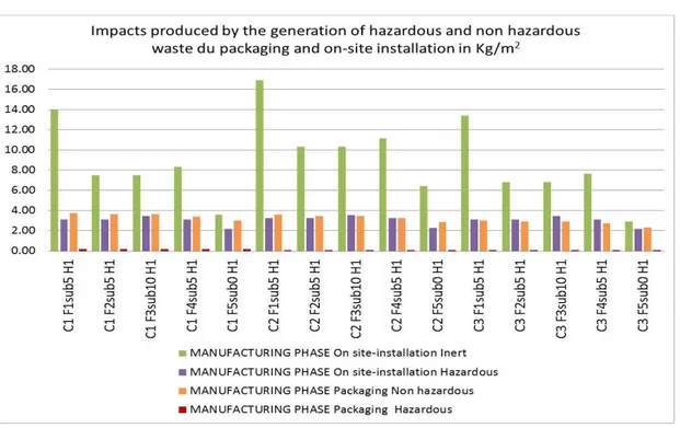
(24) Wate consumption in m3 by usable surface of dwelling. 0.06. 0.05. 0.04. 0.03. 0.02. 0.01. C3 F5sub0 H3. C3 F4sub5 H3. C3 F2sub5 H3. C3 F3sub10 H3. C3 F1sub5 H3. C2 F5sub0 H3. C2 F4sub5 H3. C2 F2sub5 H3. C2 F3sub10 H3. C2 F1sub5 H3. C1 F5sub0 H3. C1 F4sub5 H3. C1 F2sub5 H3. C1 F3sub10 H3. C1 F1sub5 H3. C3 F5sub0 H2. C3 F4sub5 H2. C3 F2sub5 H2. C3 F3sub10 H2. C3 F1sub5 H2. C2 F5sub0 H2. C2 F4sub5 H2. C2 F2sub5 H2. C2 F3sub10 H2. C2 F1sub5 H2. C1 F5sub0 H2. C1 F4sub5 H2. C1 F2sub5 H2. C1 F3sub10 H2. C1 F1sub5 H2. C3 F5sub0 H1. C3 F4sub5 H1. C3 F2sub5 H1. C3 F3sub10 H1. C3 F1sub5 H1. C2 F5sub0 H1. C2 F4sub5 H1. C2 F2sub5 H1. C2 F3sub10 H1. C2 F1sub5 H1. C1 F5sub0 H1. C1 F4sub5 H1. C1 F2sub5 H1. C1 F3sub10 H1. C1 F1sub5 H1. 0.00. Figure 7. Comparison of the impact generated by the water consumption of the different construction solutions in the manufacturing phase These data do not seem to be significant compared with the mean water consumption per inhabitant and day in Spanish homes, which is around 154 litres [43 45]. Nevertheless, water has an economic, social and environmental value, and therefore any public or private intervention must take this threefold dimension into account. - As regards the generation of inert and non-hazardous waste, the solutions that combine a lightweight façade with an inverted roof C3F5 are those that generate less waste (Figure 8). The difference between the solution that generates the most waste, C2F1H1 (23.75kg), and the solution that generates the least waste, C3F5H1 (7.43kg), is 16.32 kg, that is, 68.7% less. In absolute terms, adopting solution C3F5H1 yields a saving of 16.32 kg (0.016 metric tons) of inert and non-hazardous waste per m2 of usable floor area in the manufacturing phase.. 24.

(25) Figure 8. Comparison of the impact due to the waste generated by the different building solutions 6. Conclusions The regression model has allowed us to establish the weight of each of the explanatory variables in the impact due to the heating consumption related with the building envelope during the use phase in two different scenarios: one of them under the assumption of a low energy user, with low purchasing power, and the other, under the assumption of a high energy user with relatively high purchasing power. It is observed that the influence of some variables such as the climatic zone plays a very important role in the result. The weight of the envelope is also important although some elements used in it, such as the roofs, do not give rise to such notable alterations in the consumptions as the façades. The results obtained show that, on analysing the influence of the user on heating consumption in continental climate zones, they vary with respect to the predicted value, from 5% when the. 25.

(26) user is not very energy demanding up to over 53% when they are very high energy users. This means that the weight of the high energy users on the heating consumption is 35% and the relative weight of the climatic zone predicted by the regression model obtained by the energy simulation programs decreases from 80% to 54%. Water consumption also displays important relative variations depending on the type of envelope, whereas the generation of inert waste shows significant variations in the manufacturing and installation phase. Nevertheless, in all cases the interaction of the user may be concealing the result by substantially modifying the value of the impact during the use phase. As a general conclusion, it could be said that the designer can help contribute to reducing the actual impact throughout the life cycle of both new and refurbished buildings without diminishing the required conditions of comfort by making an appropriate choice of building solutions that help lessen the impacts. The gap between prediction and actual measurement of the impacts produced can be reduced by taking into account user interaction and selecting alternative types of envelope that help reduce the energy demand of the building regardless of the intervention of the user. Acknowledgments The authors gratefully acknowledge the financial support from the Spanish Ministry of Economy and Competitiveness, project BIA2013-44001-R: Integrated design protocol for social housing retrofit and urban regeneration.. 26.

(27) References Alías, H., Jacobo, G. Construcción sostenible. Materiales de construcción energética y ambientalmente eficientes en el nordeste de Argentina. Ciudades para un futuro más sostenible. 2008, Boletín CF+S 3 5. 2008, ISSN: 1578-097X. Alonso, C., Oteiza, I., García, J. Criterios para la reducción de emisiones de gases de efecto invernadero en el proyecto de fachadas de edificios de Viviendas. In II Congreso Nacional Investigación en Edificación. ISBN: 978-84-2844-693-8. Madrid, 2010. Allouhi, A., El Fouih,Y., Kousksou,T., Jamil, A., Zeraouli, Y. Mourad, Y. Energy consumption and efficiency in buildings: current status and future trends. Journal of Cleaner Production. 2015, Volume 109, 16, pp 118–130 Blázquez, T.; Suárez, R.; Sendra, J. J. Towards a calibration of building energy models: A case study from the Spanish housing stock in the Mediterranean climate. Informes de la Construcción. 2015, 67, 540: e128, doi: http://dx.doi.org/10.3989/ic.15.081. Burman, E.; Mumovic, D.; Kimpian, D. Towards measurement and verification of energy performance under the framework of the European directive for energy performance of buildings. Energy. 2014, 77, 153 e163. Dronkelaar, C.; Dowson, M.; Spataru, C.; Mumovic, D. (2016). A Review of the Regulatory Energy Performance Gap and Its Underlying Causes in Non-domestic Buildings. Frontiers in mechanical engineering. 2016; http://dx.doi.org/10.3389/fmech.2015.00017 Estress Consultores. Potencial de ahorro energético y de reducción de emisiones de CO2 del parque residencial existente en 2020. WWF/Adena (Madrid), 2010, España.. 27.

(28) Gonzalo, G., Ledesma, S., Nota, V., Martínez, C., Cisterna, S., Quiñónez, G., Márquez, G., Tortonese, A., Garay, A. Determinación y análisis de los requerimientos energéticos para el acondicionamiento térmico de un prototipo de vivienda ubicada en San Miguel de Tucumán. Revista Avances en Energías Renovables y Medio Ambiente. 2000, 4. Gustavsson, L., Joelsson, A. Life cycle primary energy analysis of residential buildings. Energy and Buildings. 2009, 42, 210–220 Haas, R.; Biermayr, P. The rebound effect for space heating Empirical evidence from Austria. Energy Policy. 2000, 28, (6-7), 403-410. Hernández Moreno, S. Aplicación de la información de la vida útil en la planeación y diseño de proyectos de edificación. Acta Universitaria. 2011, 21, (2), 37-42. Universidad de Guanajuato. Mexico. Hernandez-Sanchez, J.M. Consumo energético y emisiones asociadas del sector residencial”. International Congress on Project Engineering. In 15th International Congress on Project Engineering. Asociación Española de Ingeniería de Proyectos, Huesca, Spain, 2012. Herrando M; Cambra D; Navarro M; de la Cruz L; Millán G; Zabalza I. Energy performance certification of faculty buildings in Sapin: the gap between estimated and real energy consumption. Energy Conversion and Management. 2016 In Press. Published online May 2016dom. 2015. Huedo, P. La evaluación del impacto ambiental de la envolvente del edificio como herramienta de apoyo en fase de diseño aplicada a viviendas, PhD Dissertation, Universitat Jaume I, Castellón, Spain, 2014.. 28.

(29) Huedo, P., Mulet, E., Lopez-Mesa, B.. Development of an assessment tool for building. envelope retrofit based on environmental indicators. In The sustainable renovation of buildings and neighbourhoods; Mercader-Moyano P. Ed.; Bentham Science Publishers: Seville 2015; pp 81-102. Huedo, P., Mulet, e. Lopez-Mesa, B., (2016). “A model for the sustainable selection of building envelope assemblies”. Journal title: Environmental Impact Assessment Review 57 pp. 63-77. PII: S0195-9255(15)00121-3 http://dx.doi.org/10.1016/j.eiar.2015.11.005. Iyer-Raniga, U., Wong J.P.C. Evaluation of whole life cycle assessment for heritage buildings in Australia. Building and Environment. 2012, 47, 138-149. KTH + all partners’ contributions. Enslic Building. Guidelines for LCA Calculations in early design. phases. Energy. Saving. through. Promotion. of. Life. Cycle. Assessment.. EIE/07/090/SI2.467609; Intelligent Energy Europe, 2010; https://ec.europa.eu/energy/intelligent/ projects/sites/iee-projects/files/projects/documents/enslic_building_guidelines_for_lca_ calculations_en.pdf. López-Mesa, B.; Palomero, J.I.; Ortega, A.; del Amo, A. La rehabilitación y la mejora de la eficiencia energética de la vivienda social a examen. Obsolescencia de la envolvente térmica y acústica de la vivienda social de la postguerra española en áreas urbanas vulnerables. El caso de Zaragoza. Monografías de la Revista Aragonesa de Administración Pública. 2013, XV, 283-319. ISSN 1133-4797 Menezes, C.; Cripps, A.; Bouchlaghem, D.; Buswell, R. Predicted vs. actual Energy Performance of Non-Domestic Buildings. In Third International Conference on Applied Energy. Perugia, Italy 2011.3, 89-102, doi: 10.3989 / ic. 11.067.. 29.

(30) Norford, L. K.; Socolow, R. H.; Hsieh, E. S.; Spadaro, G. V. Two-to-one discrepancy between measured and predicted performance of a ‘low-energy’ office building: insights from a reconciliation based on the DOE-2 model. Energy and Buildings. 1994, 21, 121-131. Mithraratne, N. and Vale, B. Life cycle analysis model for New Zealand houses. Building and Environment. 2004, 39, 483-492. Ortiz, O., Bonnet, C., Bruno, J., Castells, F. Sustainability based on LCM of residential dwellings: A case study in Catalonia, Spain. Building and Environment. 2009, 44, 584-594. Nan Li N.; Yang Z.; Becerik-Gerber B.; Tang C.; Chen N. Why is the reliability of building simulation limited as a tool for evaluating energy conservation measures? Applied Energy. 2015, 159, 196-205. Ruá, M.J., Vives, L., Civera, V., Lopez-Mesa, B. Aproximación al cálculo de la eficiencia energética de fachadas ventiladas y su impacto ambiental. In Actas del XI Congreso mundial de la calidad del azulejo y del pavimento cerámico QUALICER, Castellón, 2010. Sendra Salas, J.J.; Domínguez Amarillo, S.; León Rodríguez, Á. L.; Bustamante Rojas, P. Intervención energética en el sector residencial del sur de España: retos actuales. In Actas del I Congreso Internacional y III Congreso Nacional de Construcción Sostenible y Soluciones Ecoeficientes, Sevilla, Spain 2013, 275-286. UNE-EN 832/2000. Comportamiento térmico de los edificios. Cálculo de las necesidades energéticas para calefacción. Edificios residenciales. Verbeeck, G.; Hens, H. Life cycle inventory of buildings: a calculation method. Building and Environment. 2009, 45(4), 1037-1041.. 30.

(31) Villar-Burke, R., Jiménez-González, D., Larrumbide, E., Tenorio, J.A. Impacto energético y emisiones de CO2 del edificio con soluciones alternativas de fachada. Informes de la Construcción. 2014, 66 (535): e030, doi: http://dx.doi.org/10.3989/ic.12.085. Wadel, G., López, F., Sagrera, A., Prieto, J. Refurbishment considering environmental impact reduction targets: a test case for a multiple-family dwelling in the area of Playa de Palma, Mallorca. Informes de la Construcción. 2011, 6. Wilde, P. The gap between predicted and measured energy performance of buildings: a framework for investigation. Automation in construction. 2014, 41, 40-49 Xexakis, G.; Dobbelsteen, A. The Gap between Plan and Practice: Actual energy performance of the zero-energy refurbishment of a terraced house Delft University of Technology. In Proceedings of Architecture and Resilience on the Human Scale: Cross-Disciplinary Conference. The School of Architecture, University of Sheffield: Sheffield, United Kingdom. 2015. Zabalza, I., Aranda, A., Scarpellini, S. Life cycle assessment in buildings: State-of-the-art and simplified LCA methodology as a complement for building certification. Building and Environment. 2009, 44, 2510-2520. 31.

(32)