Commodity and asset pricing models : an integration

Texto completo

(1)PONTIFICIA UNIVERSIDAD CATOLICA DE CHILE ESCUELA DE INGENIERIA. COMMODITY AND ASSET PRICING MODELS: AN INTEGRATION. IVO ANDRES KOVACEVIC BUVINIC. Thesis submitted to the Office of Research and Graduate Studies in partial fulfillment of the requirements for the Degree of Master of Science in Engineering Advisor: GONZALO CORTAZAR SANZ. Santiago, Chile, (July, 2013)  2013, Ivo Kovacevic.

(2) PONTIFICIA UNIVERSIDAD CATOLICA DE CHILE ESCUELA DE INGENIERIA. COMMODITY AND ASSET PRICING MODELS: AN INTEGRATION. IVO ANDRES KOVACEVIC BUVINIC. Members of the Committee: GONZALO CORTÁZAR ARTURO CIFUENTES BONIFACIO FERNÁNDEZ NICOLÁS MAJLUF. Thesis submitted to the Office of Research and Graduate Studies in partial fulfillment of the requirements for the Degree of Master of Science in Engineering Santiago, Chile, (July, 2013).

(3) ACKNOWLEDGMENTS In first place I would like to thank professor Gonzalo Cortazar for his guidance, support, time and goodwill. Without his wise advice this thesis would hardly come close to what it is. I would also like to thank professor Eduardo Schwartz for helping in this work with his wide experience. To both of them I owe the inception of this research topic and I shall always be grateful for trusting in me to develop it. Secondly, my deepest gratitude to the entire RiskAmerica-FINlabUC team. In particular, Hector Ortega for participating and supporting this thesis from day one, Hernán Morales for his enormous help in the empirical implementation of this work and Rodrigo Lártiga for introducing me to stochastic calculus. I also thank the financial support of (1) CONICYT through their Fondecyt 1130352 project and (2) FinanceUC. Finally, I would like to thank my family for providing me with the best education that one can dream of and for putting up with my long faces and mood changes when the end of this thesis seemed far away. Thanks to them and to Cami‟s support, encouragement, advice and joy this process was a great experience.. ii.

(4) TABLE OF CONTENTS ACKNOWLEDGMENTS ........................................................................................... ii TABLE OF CONTENTS ............................................................................................ iii LIST OF FIGURES ..................................................................................................... v LIST OF TABLES ..................................................................................................... vii ABSTRACT .............................................................................................................. viii RESUMEN.................................................................................................................. ix 1.. ARTICLE BACKGROUND .............................................................................. 1 1.1. Introduction ................................................................................................ 1 1.2. Main Objective ........................................................................................... 2 1.3. Literature Review ....................................................................................... 3 1.3.1. Basics about Risk-Neutral Valuation, Risk Premiums and Expected Spot Prices ....................................................................................... 3 1.3.2. Stochastic Models of Commodity Prices ......................................... 5 1.3.3. Classic Asset Pricing Models .......................................................... 6 1.4. Future Research .......................................................................................... 8. 2.. COMMODITY AND ASSET PRICING MODELS: AN INTEGRATION ...... 9 2.1. Evidence on the Financialization of Commodity Futures Markets .......... 11 2.1.1. Changes in Positions and Volume ................................................. 12. iii.

(5) 2.1.2. Changes in Price Dynamics ........................................................... 18 2.2. Some Alternative Approaches for Modeling Prices................................. 22 2.3. A Simple Methodology for Integrating Commodity and Asset Pricing Models ...................................................................................................... 25 2.3.1. First Step: Estimation of expected futures returns using an asset pricing model ................................................................................. 26 2.3.2. Second Step: Derivation of the parameter restrictions on the commodity pricing model .............................................................. 29 2.3.3. Third Step: Estimation of the commodity pricing model satisfying the parameter restrictions ............................................................... 34 2.4. Implementation and Results ..................................................................... 36 2.4.1. Data ............................................................................................... 36 2.4.2. Parameter Results .......................................................................... 39 2.4.3. Model Fit ....................................................................................... 42 2.5. Conclusion................................................................................................ 46 REFERENCES........................................................................................................... 49 APPENDIXES ........................................................................................................... 57 Appendix A: CFTC Data Processing for Investor Type Distribution ........................ 58 Appendix B: Expected Futures Return for an N-Factor Model ................................. 59. iv.

(6) LIST OF FIGURES Figure 2-1: Five year Expected Spot and Futures prices for Copper using the Schwartz and Smith (2000) model. ......................................................................... 9 Figure 2-2: Crude Oil WTI Open Interest (NYMEX). .......................................... 12 Figure 2-3: Wheat Open Interest (CBOT). ............................................................ 12 Figure 2-4: Copper Open Interest (COMEX)........................................................ 13 Figure 2-5: Transaction Volume for Oil................................................................ 14 Figure 2-6: Transaction Volume for Copper. ........................................................ 14 Figure 2-7: Daily Transaction Volume for ETFS All Commodities DJ-AIGCISM (AIGC)................................................................................................................... 15 Figure 2-8: Daily Transaction Volume for ETFS Copper (COPA). ..................... 15 Figure 2-9:. Crude Oil WTI Distribution of Positions by Trader Category. (NYMEX). ............................................................................................................. 17 Figure 2-10: Wheat Distribution of Positions by Trader Category (CBOT). ........ 17 Figure 2-11: Copper Distribution of Positions by Trader Category (COMEX). ... 18 Figure 2-12: β Evolution for Oil............................................................................ 19 Figure 2-13: β Evolution for Copper. .................................................................... 20 Figure 2-14: WTI Oil (NYMEX) Futures Term Structure .................................... 37. v.

(7) Figure 2-15: Copper (COMEX) Futures Term Structure ...................................... 38 Figure 2-16: Expected market risk premium from Graham and Harvey (2012). .. 38 Figure 2-17: Copper Futures (grey) and Expected Spot Prices (black) for 12-202011. ...................................................................................................................... 44 Figure 2-18: Oil Futures (grey) and Expected Spot Prices (black) for 12-20-2011. ............................................................................................................................... 45 Figure 2-19: Five-year Copper Futures (grey) and Expected Spot Prices (black) for 2009-2012. ............................................................................................................. 45 Figure 2-20: Five-year Oil Futures (grey) and Expected Spot Prices (black) for 2009-2012. ............................................................................................................. 46. vi.

(8) LIST OF TABLES Table 2-1: Copper estimated parameters, standard deviation (S.D) and t-Test. 20012006 time window. ........................................................................................................... 40 Table 2-2: Copper estimated parameters, standard deviation (S.D) and t-Test. 20062011 time window. ........................................................................................................... 41 Table 2-3: Copper estimated parameters, standard deviation (S.D) and t-Test. 20092012 time window. ........................................................................................................... 41 Table 2-4: Oil estimated parameters, standard deviation (S.D) and t-Test. 2001-2006 time window. .................................................................................................................... 41 Table 2-5: Oil estimated parameters, standard deviation (S.D) and t-Test. 2006-2011 time window. .................................................................................................................... 42 Table 2-6: Oil estimated parameters, standard deviation (S.D) and t-Test. 2009-2012 time window. .................................................................................................................... 42 Table 2-7: Copper In-Sample and Out-of-Sample Mean Absolute Error for the three methods. Errors are calculated as percentage of the observed futures price. ................... 43 Table 2-8: Oil In-Sample and Out-of-Sample Mean Absolute Error for the three methods. Errors are calculated as percentage of the observed futures price. ................... 43. vii.

(9) ABSTRACT A simple methodology that integrates commodity and asset pricing models is presented. Given current evidence on the financialization of commodity markets, valuable information about commodity risk premiums can be extracted from asset pricing models and used to substantially improve the estimates of expected spot prices provided by current commodity price models. The methodology can be used with any pair of commodity and asset pricing models. An implementation of the methodology is presented using the Schwartz and Smith (2000) two-factor commodity price model and the CAPM. Reasonable expected spot prices are obtained without negative consequences in the model‟s fit to futures prices.. Keywords: Commodity Prices, Stochastic Dynamic Model, Financialization, RiskPremium, Expected Spot Prices. viii.

(10) RESUMEN Se presenta una simple metodología para integrar modelos de commodities y de valorización de activos. Considerando la nueva evidencia sobre la financialización de los mercados de commodities, información valiosa se puede extraer de los modelos de valorización de activos y usar para mejorar substancialmente la estimación de los precios esperados que entregan los actuales modelos de precios de commodities. La metodología se puede usar con cualquier par de modelos de commodities y de valorización de activos. Se presenta una implementación de esta metodología usando el modelo de dos factores de Schwartz y Smith (2000) junto con el CAPM. Se obtuvieron precios esperados razonables sin consecuencias negativas sobre el ajuste del modelo a los precios futuros.. Palabras claves: Precios de Commodities, Modelo Dinámico Estocástico, Financialización, Premios por Riesgo, Precios Spot Esperados. ix.

(11) 1. 1.. ARTICLE BACKGROUND. 1.1.. Introduction The work presented in this thesis is based on two observations about stochastic. models of commodity prices. First, while current models provide a satisfactory fit of futures contracts term structure, expected spot prices implied by these models often result to be highly unreasonable and unreliable. This is reflected in: i.. Differences between expected spot prices and futures prices which aren‟t justified by market expectation and classic asset pricing theories.. ii.. Poor statistical significance for the risk premium parameters, which are fundamental for the expected spot price estimation (as it will be explained in section 1.3.1). The second observation is that development done in the field of commodity price. modeling has been carried out ignoring classic asset pricing models (which relate the expected return of an asset with the market risk associated to it). While this assumption was appropriate in the past when commodity futures were not viewed as financial assets, a wide literature on the financialization of commodity markets shows that investors are starting to include these derivatives in their portfolios. In line with these observations the hypothesis of this thesis is that, due to the recent financialization of commodity markets, information can be obtained from asset pricing models and used to improve the estimation of risk premiums and therefore of the expected commodity spot prices. The rest of this work structured as follows. Section 1.2 presents the main objectives; section 1.3 presents a short literature and conceptual review that serves as a theoretical framework and section 1.4 states two lines of further research. Following this, Section 2.

(12) 2. contains the main article of this thesis. Within this, Section 2.1 presents evidence on the financialization of commodity futures markets, Section 2.2 provides a short review on different commodity and asset pricing models, Section 2.3 describes the integration methodology that we propose and Section 2.4 presents the results of implementing the methodology for Copper and Oil futures. Finally, Section 2.5 concludes. 1.2.. Main Objective The goal of this thesis is to propose a methodology to add information from asset. pricing models into stochastic models of commodity prices and by doing so obtain risk premiums and expected spot prices that are consistent with the former model. The basic idea is to achieve this by adding a set of restrictions to the estimation process of the commodity model so that the estimated parameters are forced to reflect the results from the selected asset pricing model. An important feature of the methodology is that it ought to be general. This means that it must be compatible with any pair of commodity and asset models. This will allow practitioners interested in applying the proposed methodology to use the models that they see fit and therefore the usefulness of this procedure will not be restricted by the goodness of the underlying models. Finally, a second objective is to perform an implementation of the methodology with a specific pair of commodity and asset pricing models. This is aimed to compare the results of using the proposed methodology with those obtained from an estimation of the same commodity model without incorporating the information from the asset pricing model. It is expected that by using the integration methodology the model‟s ability to fit futures contracts will not be significantly affected, and at the same time results obtained for risk premiums and expected spot prices will be consistent with the asset pricing model and therefore more reasonable and robust..

(13) 3. 1.3.. Literature Review. 1.3.1. Basics about Risk-Neutral Valuation, Risk Premiums and Expected Spot Prices Risk-neutral valuation is central in modern asset pricing theory and has been used since Black and Scholes (1973) applied it to equity contingent claims. The procedure arises from assuming that assets are priced in such a way that arbitrage opportunities are ruled out. This pricing method states that derivatives1 (or contingent claims) can be priced by computing the expectation of the discounted future cash flows under a risk neutral probability measure2 [Cox and Ross (1976)]. If future cash flows are uncorrelated with the risk free interest rate, valuation can be performed by first estimating the expected future cash flows under this risk-neutral measure and then discounting them by the risk free rate [Cortazar and Schwartz (1994)]. A special case of derivatives that can be priced by risk neutral valuation are futures contracts. These contracts are agreements between two parts to buy or sell an asset at a certain time in the future for a certain price (known as the futures price) [Hull (2009)]3. As it will be discussed later, these assets are the primary information used to estimate stochastic models of commodity prices.. 1. A derivative can be defined as a financial instrument whose value depends on the value of other underlying variables, which are frequently prices of other traded securities [Hull (2009)]. 2 The risk neutral measure also known as the equivalent martingale measure is a modified probability distribution under which every security earns the riskless rate without changing the set of events that receive a positive probability [Harrison and Kreps (1979)]. For further reference see Baxter and Rennie (1996) or Cochrane (2005). 3 It‟s also important to mention that unlike forward contracts, futures are generally traded on an Exchange while forward contracts are over the counter (OTC) agreements..

(14) 4. Cox et al. (1981) shows that the price of a futures contract is given by the expected value of the spot price under the risk-neutral probability measure (Q-measure). Formally, the price at time t for a futures contract maturing at time t+T (. ) is given. by: ( where. ). is the spot price at time t+T and. (1.1) ( ) denotes the expectation at time t. under the Q-measure. Equation 1.1 provides a relation between the observed futures price and the expectation under the risk adjusted measure, but does not provide information about the expected value under the physical or true measure. In order to relate the risk neutral measure with the physical measure a risk premium parameter ( ) must be introduced. The risk premium is the excess return over the risk free rate that the owner of the commodity obtains in compensation for the commodity risk. Following Heath (2013), the relation between the futures price and the expected spot price is given by: ( where. ). (1.2). ( ) denotes the expectation under the real or physical measure.. Equation 1.2 implies that future prices represent expected spot prices only if. is. zero. If the risk premium is different from zero a reliable estimate of this parameter must be obtained in order to adjust the futures price and get the expected spot price as explained by Equation 1.2. Current stochastic models of commodity prices (which will be discussed in more detail in sections 1.3.2 and 2.2) are accurate in estimating the dynamics under the risk neutral measure, but fail to provide a reasonable estimation of the probability.

(15) 5. distribution under the physical measure. This is a consequence of the mentioned problems regarding risk premiums and is the issue due to be solved with the proposed methodology. Finally a question that could be raised here is why is the expected spot price important if one can use futures prices as the expected value under the Q-measure and then perform valuation under the risk-neutral framework? This question will be answered in section 2. 1.3.2. Stochastic Models of Commodity Prices Most stochastic models of commodity prices are composed of state variables and model parameters. The state variables are the stochastic components of the model and are generally time-varying latent (unobservable) variables which try to capture the effect of the various factors that may influence commodity price dynamics in a complex macroeconomic system [Naranjo (2002)]. In turn, the mentioned parameters are the structural component of the model and determine the stochastic behavior of these state variables. By specifying a model in this manner, it can be used to obtain the probability distribution of the commodity price and therefore they become fundamental for valuation [Schwartz (1997)] and for risk management purposes. A further review of commodity models currently available in the literature can be found in section 2.2. Using the fact that futures prices are the expected value under the risk neutral measure, close form formulas for the futures price can usually be found for each of these models. Based on these expressions and observed futures prices, the unobservable state variables can be obtained for a certain set of parameters by simply inverting the futures pricing formula. Now, as the number of futures prices available for each date is generally higher than the number of state variables, it must be assumed that the observed futures prices have some degree of measurement error [Cortazar and Naranjo (2006)] an.

(16) 6. therefore suitable econometric techniques must be used to estimate the state variables and the model‟s parameters. A procedure widely used in the related literature to estimate this kind of models is the Kalman filter [for example: Schwartz (1997), Schwartz and Smith (2000) and Cortazar and Naranjo (2006)]. The Kalman filter is a recursive method that addresses the issues of having non observable variables and measurement errors associated with the observable data. In combination with Maximum Likelihood, It allows estimating these state variables and the model‟s parameters from a wide range of futures contract without having to select a subset of them which would imply losing a portion of the available information. Section 2.3.3 presents in more details the application of this technique for the case of the empirical implementation that is presented in this thesis. 1.3.3. Classic Asset Pricing Models Asset Pricing Literature deals with the relation of risk and return. The basic concept is that riskier securities should have a higher expected return. While different models consider different risk factors, the positive risk-return relation is a constant across them all. Modern Asset Pricing Theory has its starting point with the Capital Asset Pricing Model (CAPM) of Sharpe (1964), Lintner (1965) and Black (1972). Fama and French (1992) describe the main aspects of the model as follows: “The central prediction of the model is that the market portfolio of invested wealth is mean-variance efficient in the sense of Markowitz (1959). The efficiency of the market portfolio implies that (a) expected returns on securities are a positive linear function of their market. (the slope in the regression of a security’s return on the market’s. return), and (b) market. suffice to describe the cross-section of expected returns.”.

(17) 7. This implies that, in the context of the CAPM, the risk of an asset is described by its market , being this the only risk measure relevant for determining an assets expected return. A second asset pricing model is the Intertemporal Capital Asset Pricing Model (ICAPM) formulated by Merton (1973). In this model, investors are not only worried about the portfolio payoff, but also about the opportunities they would have to consume or invest those payoffs. This implies that risk is associated with a series of economic state variables, not only with the market‟s return [Fama and French (2004)]. Another multifactor model is provided by the Arbitrage Pricing Theory (APT) of Ross (1976). While similar to the ICAPM, the fundamental difference is in the inspiration for the factors as the APT starts with factor analysis to find portfolios that characterize common movement while the ICAPM suggest starting by thinking about the state variables [Cochrane (2005)]. This results in the APT having the fundamental problem of not providing an economic interpretation of the factors [Fama and French (1991)]. Probably the most popular specification of a multifactor model is that of Fama and French (1993). This work identifies five common risk factors in the returns of stocks and bonds4. Three of these associated to stock returns and the other two associated to bonds5. While most of these models where though and tested for stocks (or bonds like in Fama and French (1993)), they have also been applied to commodity investments. A short review of this literature is presented in section 2.2. It‟s important to note here that applications of these models to commodities are generally performed on commodity. 4. Fama and French (1993, 1996) also propose a three factor model for stock returns considering the three stock-related factors. 5 The factors asociated to bonds also have influence on stock returns..

(18) 8. futures prices and not on spot prices. As it was mentioned above, futures contracts are just agreements between two parts to buy a certain asset in the future. As the futures prices is set so that there are no arbitrage opportunities, the value of a futures position is zero at origination and requires no capital investment by any of the two parts entering the agreement [Bessembinder (1992)]. Because of this, commodity futures return (computed as log differences or percentage changes of consecutive futures prices) can‟t be interpreted as a typical return. It is simply a price change, not the return gained by an investor over a certain initial capital investment (because such an investment does not exist in this case). This has important implications for the application of asset pricing models as it will be showed in section 2.3. 1.4.. Future Research The results presented in this thesis correspond to a specific pair of commodity and. asset pricing models. Therefore, as the methodology is general and can be used with any choice of the two kinds of models, a first line of future research should be to test the methodology with other combination of them. As it will be explained in more detail in section 2, the implementation presented corresponds to the Schwartz and Smith (2000) two-factor model and the CAPM as the commodity and asset pricing models respectively. A natural step would be to apply the methodology with models that incorporate more factors, for example a three-factor commodity model in the spirit of Cortazar and Naranjo (2006) and a multifactor asset pricing model like the one presented in Erb and Harvey (2006). A second line of research that could be developed is to improve the estimation methodology. One important aspect to attack is finding a way to perform the estimation of the commodity and asset pricing model in a joint manner and not in separate estimations as it is performed in this work. This would not only make the procedure more elegant, but it would also solve some statistical difficulties that arise from this fact..

(19) 9. 2.. COMMODITY AND ASSET PRICING MODELS: AN INTEGRATION Stochastic models of commodity prices have evolved considerably during recent. years. Using multiple factors, different specifications and modern estimation techniques, these models have been able to accurately fit commodity futures‟ term structures and their dynamics. While this fit implies that the parameters that determine the risk-adjusted process seem adequate, risk premiums (which affect the dynamics under the physical measure) are far from robust. Thus the expected spot prices obtained from these models may be highly unreliable. To illustrate this issue consider the model presented in Schwartz and Smith (2000). Calibrating this model with COMEX copper data from January 2009 to February 2012, the five-year futures and expected five-year spot prices for each date are presented in Figure 2-1.. It can be seen that for this example results are unreasonable, as it is very. unlikely for expected spot prices in five years to be around 5 times the corresponding five-year futures price today, as shown in the figure. 2500 Expected Spot Future. Price (¢/Pound). 2000. 1500. 1000. 500. 0 01-09. 01-10. 01-11. 01-12. 01-13. Figure 2-1: Five year Expected Spot and Futures prices for Copper using the Schwartz and Smith (2000) model..

(20) 10. It is well known that expected spot and futures prices should differ only on the risk premiums since futures prices are expected spot prices under the risk neutral measure. Thus, if these risk premiums are not well estimated, even though futures prices may not be affected, expected spot prices under the physical (true) measure will be6. Under a risk neutral framework, asset valuation can be done using futures prices to estimate cash flows and then discounting them at the risk free rate. This makes future expected spot prices unnecessary for valuation purposes. While this is true, the commodity price distribution under the physical measure is still important. The reason for this is twofold. First, the true distribution is useful for purposes other than valuation, for example, for risk management (i.e. calculations of the Value at Risk). Second, many practitioners still do not use the risk neutral approach for valuing natural resource investments, but instead use commodity price forecasts and then discount the expected cash flows at the weighted average cost of capital 7. Thus, not only the risk adjusted process is of interest for users of commodity models, but also the dynamics under the physical measure. Moreover, the fact that commodity models may provide such unreasonable estimations of expected spot prices limits the credibility and practical use of these commodity models altogether.. 6. In an independent work, Heath (2013) also finds that a futures panel is well suited for estimating the cost of carry, relevant for futures prices, but not the risk premiums, required for expected spot prices, as will be described later. 7. The International Valuation Standards Council (IVSC) released the discussion paper Valuation in the Extractive Industries in July 2012. Different questions about valuation methodologies where stated in this paper which industry participants were invited to answer. These answers where published and can be accessed at http://www.ivsc.org/comments/extractive-industries-discussion-paper. Respondents include the Valuation Standards Committee of the SME, The VALMIN Committee, the CIMVal committee and the American Appraisal Associates among others. Most of the respondents stated that their main method of valuation was a discounted cash flow analysis (DCF) using various methods of price forecasting. For the discount factor the most widely used method was a weighted average cost of capital (WACC) based on the Capital Asset Pricing Model (CAPM)..

(21) 11. There is a separate strand on the finance literature that deals with asset pricing models which has been largely ignored in the commodity pricing literature.. One. explanation for this may be that commodity futures in the past were generally traded by non-financial institutions and therefore didn‟t behave as a classic financial asset. However, this has changed in recent years. Commodities have attracted a growing interest from the financial world and have started to be viewed as an asset class on their own. This issue has generated a large literature on the financialization of commodity markets. While the debate is still ongoing, there is considerable empirical evidence that commodity futures are behaving more like classic financial assets and are being included as an asset class in portfolio allocation algorithms. Therefore, considering the rise of commodities as an asset class and their financialization, commodity pricing models should not ignore information about risk premiums that could be obtained from classic asset pricing models. This paper proposes to integrate these two types of models by extracting information from the latter and using it in stochastic commodity pricing models. We show that it is possible to obtain more reliable estimates not only of futures prices but also of expected spot prices, thus making commodity models more credible. 2.1.. Evidence on the Financialization of Commodity Futures Markets Extensive debate has emerged recently about the financialization of commodity. markets. According to Henderson et al. (2012) financialization is the process by which the financial sector has gained influence relative to the real sector over the behavior of commodity prices. The authors point out two strands of the literature about financialization: one which describes changes in the trading and positions of investors in the commodity markets, while the other one analyzes changes in the price dynamics that might be explained by the new inflow of financial investors..

(22) 12. 2.1.1. Changes in Positions and Volume Commodity futures markets have experienced big changes since the beginning of the 21st century. Open interest in commodity futures markets were significantly larger in 2010 than those observed a decade earlier [Büyüksahin and Robe (2012b)]. Figures 2-2 through 2-4 show the open interest for three commodities: WTI Oil, Wheat and. Open Interest (Thousands). Copper which grew 212%, 270% and 99%, respectively, during the decade. 1.800 1.600 1.400 1.200 1.000 800 600 400 200. Date. Open Interest (Thousands). Figure 2-2: Crude Oil WTI Open Interest (NYMEX). Source: CFTC. 600 500 400 300 200. 100. Date Figure 2-3: Wheat Open Interest (CBOT). Source: CFTC.

(23) Open Interest (Thousands). 13. 180 160 140 120 100 80 60 40 20. Date Figure 2-4: Copper Open Interest (COMEX). Source: CFTC. Figure 2-5 and Figure 2-6 show the traded volume for the three shortest maturity contracts between 2000 and 2012 for oil and copper, respectively. Both figures show a relatively constant volume for the first years of the decade and a sharp increasing trend starting in 2007 for oil and in 2009 for copper. Similar behavior can be observed for Commodity Exchange Traded Funds (Commodity ETF).. Figure 2-7. and. Figure 2-8. show. transaction volume for two different commodity ETF‟s. Again in line with the financialization process, both figures show very low volume for the first years and a significantly higher volume since mid- 2009..

(24) 14. 1200000 1100000 1000000 900000 800000 700000 600000 500000 400000 300000 200000 100000 0. Figure 2-5: Transaction Volume for Oil. Traded volume for the three shortest contracts available for each day. Source: Bloomberg.. 100000 90000 80000 70000 60000 50000 40000 30000. 20000 10000 0. Figure 2-6: Transaction Volume for Copper. Traded volume for the three shortest contracts available for each day. Source: Bloomberg..

(25) 15. 2500000 2250000 2000000 1750000 1500000 1250000 1000000 750000 500000 250000 0 28-09-2006. 28-09-2007. 28-09-2008. 28-09-2009. 28-09-2010. 28-09-2011. Figure 2-7: Daily Transaction Volume for ETFS All Commodities DJ-AIGCISM (AIGC). This ETF tracks the DJ-AIG Commodity Index SM.. 1000000 800000 600000 400000 200000 0 28-09-2006. 28-09-2007. 28-09-2008. 28-09-2009. 28-09-2010. 28-09-2011. Figure 2-8: Daily Transaction Volume for ETFS Copper (COPA). This ETF tracks the DJ-AIG Copper Sub-Index SM.. This increase in commodity futures market activity can be partly explained by the use by financial institutions and investors from the financial sector of commodities as a new asset class to be included in their investment portfolios. New interest for investing in commodities has been motivated in part by empirical research that found positive historical returns together with low or even slightly negative equity-commodity correlations and positive inflation-commodity correlations [Gorton and Rouwenhorst (2006), Erb and Harvey (2006)], increasing the appeal of these assets..

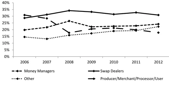
(26) 16. Not only did open interest in commodity futures market increase, but also the proportion of participants from the financial sector taking positions on commodity futures rose sharply. For example, the market share of financial traders in WTI oil market went from less than 20% in 2000 to more than 40% in 2010 [Büyüksahin and Robe (2012a)]. This change in investor-type distribution is largely explained by increased commodity index funds investments [Irwin and Sanders (2011)] and money managers (hedge funds) positions [Büyüksahin and Robe (2012b)]. Some additional information that has been made public by the Commodity Futures Trading Commission (CFTC) is summarized in Figures 2-9 to 2-11. These figures show how the positions in the corresponding commodity are distributed between different types of investors8. Even though this information only dates back to 20069 some interesting trends can still be observed. For WTI oil, positions by the “producer/merchant/processor/user” category dropped from more than 30% in 2006 to less than 18% in 2012. This drop had its counterpart in the other three categories that have seen their share grow during the same time period. A similar trend can be seen for wheat. futures.. Even. though. for. copper. the. drop. in. the. “producer/merchant/processor/user” category isn‟t as sharp as for the other commodities, the increase in the “money manager” positions is considerable going from around 16% in 2006 to more than 24% in 2012. All of this clearly points towards the idea of the financialization of commodities, as financial institutions are having a higher presence in commodity markets.. 8. Further explanation on how the raw CFTC data was processed to obtain these figures is available in appendix A. 9 Other work such as the cited Büyüksahin and Robe (2012b) has non-public data available which dates further back than 2006..

(27) 17. 40% 35% 30% 25% 20% 15% 10% 5% 0% 2006. 2007. 2008. 2009. 2010. 2011. 2012. Money Managers. Swap Dealers. Other. Producer/Merchant/Processor/User. Figure 2-9: Crude Oil WTI Distribution of Positions by Trader Category (NYMEX). Source: Calculated from CFTC Data. 35% 30% 25% 20%. 15% 10% 5% 0%. 2006. 2007. 2008. 2009. 2010. 2011. 2012. Money Managers. Swap Dealers. Other. Producer/Merchant/Processor/User. Figure 2-10: Wheat Distribution of Positions by Trader Category (CBOT). Source: Calculated from CFTC Data.

(28) 18. 35% 30% 25% 20% 15% 10%. 5% 0% 2006. 2007. 2008. 2009. 2010. 2011. 2012. Money Managers. Swap Dealers. Other. Producer/Merchant/Processor/User. Figure 2-11: Copper Distribution of Positions by Trader Category (COMEX). Source: Calculated from CFTC Data. 2.1.2. Changes in Price Dynamics At the same time when changes in investor positions occurred, and perhaps because of it, there has been a change in commodity futures price behavior. In particular, four effects have been documented: increases in price volatility [Tang and Xiong (2012)]; increases in the correlation between the returns of different commodities [Tang and Xiong (2012)]; increases in the correlation of commodity returns with various market factors, such as stock market returns [Büyüksahin and Robe (2012b)]; and changes in the pricing of risk [Hamilton and Wu (2013a)] Of particular interest is the increase in the correlation between commodity and equity markets since there is a substantial change in relation to what was observed in previous studies [Gorton and Rouwenhorst (2006), Erb and Harvey (2006)] which showed that equity-commodity correlation was rather low. Until May 2008, the correlation between commodity and equity indexes had not experienced any significant.

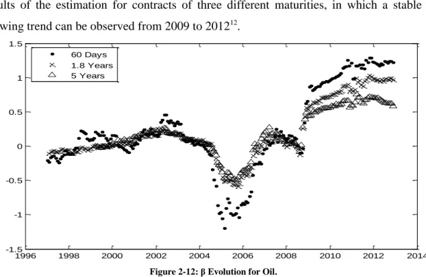
(29) 19. change, maintaining their fairly variable behavior over time [Büyüksahin et al. (2010)]10. However, in more recent work Büyüksahin and Robe (2012b) show that from September 2008 the correlation between stocks and commodities has experienced a sharp increase remaining at a high level until the end of the time window considered (year 2010). Tang and Xiong (2012) and Silvennoinen and Thorpe (2013) find similar results. This correlation increase should be reflected in the. coefficient of the Capital Asset. Pricing Model (CAPM) applied to commodity futures. A time series of. coefficients for. oil and copper are presented in Figure 2-12 and Figure 2-13, respectively. The values are obtained using a two-year rolling window of weekly returns11. The figures show the results of the estimation for contracts of three different maturities, in which a stable growing trend can be observed from 2009 to 201212. 1.5. 1. 60 Days 1.8 Years 5 Years. 0.5. 0. -0.5. -1. -1.5 1996. 1998. 2000. 2002. 2004. 2006. 2008. 2010. 2012. 2014. Figure 2-12: β Evolution for Oil. 2-year rolling window β coefficients for contracts of different maturities.. 10. On the other hand, Chong and Miffre (2010) using data that comprises the period 1980-2006, conclude that the correlation between commodities and stock indexes have declined over time. 11 Further explanations of the calculation are presented in section 2.3.1. 12. Considering the two-year rolling window the data is from 2007 to 2012.

(30) 20. 1.5. 1. 60 Days 1.8 Years 5 Years. 0.5. 0. -0.5. -1. -1.5 1996. 1998. 2000. 2002. 2004. 2006. 2008. 2010. 2012. 2014. Figure 2-13: β Evolution for Copper. 2-year rolling window β coefficients for contracts of different maturities.. There is an extensive literature that studies the linkage of investor positions and price dynamics. Empirical research in this area has reached different conclusions. Büyüksahin and Harris (2011) find little evidence that traders‟ activity caused price changes in crude oil futures market from 2000-2008. Similarly, Brunetti et al. (2011), with data for 2005-2009, conclude that positions of different types of investors (including swap dealers and hedge funds) have no effect on prices but are effective in reducing volatility. Similarly, Sanders and Irwin (2011a and 2011b) find that swap dealers and index trader‟s positions did not help predict returns for most of the commodities under study and Hamilton and Wu (2013b) conclude that there is little evidence that index-fund investing has a considerable impact on commodity futures prices. In contrast, Mou (2011), using data from 2000 to March 2010, finds out that index traders‟ activity, when rolling over between contracts of different maturities, has a significant impact on price levels. Additionally, Mayer (2012), using Granger causality tests, concludes that the positions of commodity index investments caused changes in.

(31) 21. prices for several commodities (soybeans, soybean oil, oil and copper) throughout their sample period (July 2006 - June 2009), while the positions of hedge funds only affected copper and oil during what they considered the crisis period (June 2007 - June 2008). In turn, Singleton (2012) shows that changes in spread positions of hedge funds and index traders in medium-term futures caused price changes in the period September 2006 January 2010. In terms of the correlation increase between equity and commodity futures‟ returns Büyüksahin and Robe (2012b) conclude that hedge funds‟ activity in commodity futures helps explain the rise in their correlation with equity during the 2000-2010 period. Furthermore, they find that hedge funds that actively trade in both markets are especially relevant while positions from investors outside of the hedge fund category have little explanatory power over the equity-commodity correlation. In turn, Tang and Xiong (2012) find that this correlation rises more sharply for futures belonging to indexes usually used as benchmark (GSCI y DJ-UBSCI) than for those that don‟t belong to these indices. While these last studies seem to provide solid evidence on the effects of changes in investor behavior, these findings should be taken with caution because of some problems arising from the causality tests used [Irwin and Sanders (2011)] and how index traders‟ positions are computed or approximated [Irwin and Sanders (2011, 2012), Singleton (2012)]. In summary, while debate is still ongoing about the relation between investors' positions and price levels, evidence on the influence of the financial sector over commodity-equity correlation seems to be strong, supporting the financialization of commodity futures markets and the emergence of commodities as an asset class..

(32) 22. 2.2.. Some Alternative Approaches for Modeling Prices There have been two main approaches for modeling prices and returns: Stochastic. Pricing Models, which use no-arbitrage arguments to define price dynamics, and Asset Pricing Models, which estimate risk premiums that should be earned by investors in equilibrium. The first type of models has been the main approach used for commodity futures. Several of these models have been proposed during the last decades. Their specification varies considerably depending on the number and interpretation of the state variables that model the underlying risk [Gibson and Schwartz (1990), Schwartz (1997), Schwartz and Smith (2000), Cortazar and Schwartz (2003), Cortazar and Naranjo (2006)]. These models are calibrated using futures panel data13. They assume that there are no-arbitrage opportunities in trading within these contracts and that the underlying process for commodity prices may be derived using only futures prices. These models have gained wide acceptance because of their success in accurately fitting the observed futures term structure and its dynamics. However, while the estimation of futures prices is adequate, the estimation of risk premiums may be unreasonable, such as those presented in Figure 2-1. In addition it is often the case that risk premium parameters estimated with these models are statistically insignificant. Singleton (2012) points out that commodity excess return is given by the risk premium minus the convenience yield. Because of this, an accurate model of commodity price dynamics must capture the effect of these two variables. As in Heath (2013), we argue that futures contracts data contains enough information to ensure a correct. 13. Futures prices for contracts with different maturities and dates..

(33) 23. estimation of the cost of carry14 (which is relevant for futures prices) but not necessarily of the risk premiums (which are required for obtaining expected future spot prices). Previous work with commodity models that add new information, in addition to futures prices, include Schwartz (1997) and Casassus and Collin-Dufresne (2005), which include bond prices and Geman and Nguyen (2005) that incorporate inventory data. Also Cortazar et al. (2008) and Cortazar and Eterovic (2010) formulate multicommodity models which use prices from one commodity to estimate the dynamics of another, and Trolle and Schwartz (2009) use commodity option prices to calibrate an unspanned stochastic volatility model. A second and separate approach for modeling commodity prices and returns are asset pricing models which estimate investor risk premiums. A number of different asset pricing models have been applied to commodity returns. The starting point of this line of research can be found in Dusak (1973) who studied risk premiums under the Capital Asset Pricing Model (CAPM). Dusak‟s work focused on three agricultural commodities and found. coefficients close to zero for all of them. In other related research Bodie and Rosansky (1980) estimate. coefficients for. different commodities and find that the CAPM doesn‟t hold. Carter et al. (1983) discuss the validity of Dusak‟s selection of the S&P 500 index as the market proxy and state that another index should be used. They also find systematic risk significantly different from zero (for the same contracts studied by Dusak) when. is allowed to be stochastic and it. is specified as a function of net market position of large speculators. Chang et al. (1990) finds significant systematic risk for copper, platinum and silver, differing from previous work done on agricultural commodities.. 14. The cost of carry ( ) is given by convenience yield.. , where. is the risk free rate and. is the.

(34) 24. Furthermore, Bessembinder and Chan (1992) and Bjorson and Carter (1997) find that treasury bill yields, equity dividend yields and the „junk‟ bond premium have forecasting power in various commodity future markets. Bessembinder (1992) presents results for single and multiple. models15 while Erb and Harvey (2006) apply a variation. of Fama and French (1993) five factor model to various commodities and commodity portfolios. In both works no factor is consistently significant across commodities. Bessembinder (1992) also uses his single and multiple. models to test for market. integration. He finds no statistical evidence to reject the market integration hypothesis16 while on a different test finds out that hedging pressure has an impact on commodity and currency futures but not on financial futures17. De Roon et al. (2000) show that hedging pressure on futures contracts and also hedging pressure on other markets (cross-hedging pressures) have significant influence on futures return. In more recent research Khan et al. (2008) report results for a three factor model which considers a market proxy, an inventory variable and a hedging pressure variable. The model is applied to copper, crude oil, gold and natural gas presenting mixed results. While the hedging pressure variable holds explanatory power across the four commodities, the other two variables are not statistically significant in all of them. Moreover Hong and Yogo (2010) study the predictability of commodity futures returns. They use a commodity futures portfolio composed of 30 products from the agriculture, energy, livestock and metal sectors. They find that the short rate, the yield. 15. In the single model the explanatory variable is the return on a market index while in the multiple model six macroeconomic variables are also considered besides the market index. 16 This is done by studying the uniformity of risk premiums across assets and futures with an adaptation of the traditional Fama and MacBeth (1973) methodology. He recognizes that the test performed has relatively low power. 17 The impact of hedging pressure is observed when residual risk, conditional on a hedging pressure variable, is used. This is consistent with Hirshleifer (1988).

(35) 25. spread, the aggregate basis18 and the open interest growth rate helps to predict commodity futures returns. Finally Dhume (2010) studies commodity futures returns using a consumptionbased asset pricing model developed by Yogo (2006) which extends the classic consumption CAPM (CCAPM) to include durable goods. Dhume finds out that the high correlation between commodities and durable goods consumption growth can explain commodity returns. This finding contrast with Jagannathan (1985) who found that the CCAPM (not including durable goods) was rejected for agricultural commodities. 2.3.. A Simple Methodology for Integrating Commodity and Asset Pricing Models Given the inability of commodity pricing models to provide reliable estimations of. expected spot prices, and the new relevance of asset pricing models due to the financialization of commodity markets, we propose integrating these two approaches. The methodology is divided into three steps: (i) Estimation of expected futures returns using an asset pricing model. (ii) Derivation of the parameter restrictions on the commodity pricing model required to obtain a given expected futures return (iii) Estimation of the commodity pricing model satisfying the parameter restrictions. This methodology requires choosing an asset pricing model and a commodity pricing model. To illustrate its implementation we use the CAPM as the asset pricing model, and the Schwartz and Smith (2000) model as the commodity pricing model. We use copper and oil data to perform the estimations. The methodology naturally applies to alternative choices of asset pricing models and of commodities.. 18. Interesting to note here is that the basis has been found to be related to inventory levels and to the risk premium [Gorton et al., 2013].

(36) 26. 2.3.1. First Step: Estimation of expected futures returns using an asset pricing model The basic output of an asset pricing model applied to commodity futures is the expected return of a futures contract on asset i with time to maturity T ( (. )). How. to implement this step obviously depends on the asset pricing model selected. As it was mentioned in the previous section, the implementation of the methodology that will be presented here is done considering the CAPM. In its classical form the CAPM is defined as: ( ) where risk free rate,. [ (. is the return on asset i,. ). ]. (2.1). is the return on the market portfolio,. is the systematic risk of asset i and. is the. ( ) is the expectation operator. conditional on the information available at time t. Futures contracts are a special case of assets as they represent zero investment positions. Following Chang et al. (1990) and Bessembinder (1992) the CAPM for futures contracts is defined as: ( where. ). [ (. ). ]. (2.2). is the return on the futures price for a contract on the underlying asset i. that matures at time. . Two important details about this specification are worth. mentioning. First, for a particular commodity multiple. coefficients can be estimated. depending on the time to maturity (T) of the futures contract chosen. Second, this relation implies that the expected return earned by a holder of a long position in the futures contract is only given by the expected risk premium..

(37) 27. When estimating. coefficients from Equation 2.1 the following regression is. typically run19: [ where. ]. (2.3). is the realized return of the asset for time period t,. return on the market portfolio for time period t, is an error term and. is the estimate of. is the realized. is the risk free rate at time period t,. . Also, if the CAPM holds,. should not be. statistically different from zero. However, when applied to future contracts the coefficients to be estimated are those of Equation 2.2, therefore, the following regression is estimated: [. ]. (2.4). where the same terms of Equation 2.3 can be found, with the exception that in this case time. is the realized return for time period t of a future contract that matures at ,. is an error term and. is the estimated value of. present in Equation. 2.2. Note that to perform the regression specified by Equation 2.4 a futures contract with exact time to maturity T should be available for each time period (. ).. This is not the case as one futures contract matures each month. Because of this, a rolling strategy must be followed in order to hold a contract that has an approximate maturity of T. At the end of each month the futures contract that has the closest time to maturity to the defined value T is selected. This futures contract is held for the next month and by the end of the month the same process is repeated. Once the futures. 19. For simplicity sub-index i will be dropped from the notation from this point on..

(38) 28. contract is selected, the price of this contract is used to calculate the futures return. Defining. as the price at time t of a futures contract that matures at time. , the. return is defined as the log difference of consecutive futures prices20: (. ). In addition to an estimate of the market risk premium,. [ (. ). (. ). (2.5). coefficient, an estimate of the expected ], is needed in order to use Equation 2.2.. Damodaran (2009) suggests that there are three alternative approaches to estimate the equity risk premium: (i) survey investors, managers or academics, about their expectations, (ii) use the historical premium (over a certain period of time) as the market expectation and (iii) use implied methods that try to extract the expectations from market prices or rates. For simplicity the survey approach will be used in this work. Two types of surveys are available in the literature: those that ask academics [Fernandez (2009), Welch (2001 and 2008)] and those that ask CFO‟s [Graham and Harvey (2005)]. In an unpublished work, Graham and Harvey (2012) update their 2005 work providing quarterly results for the average expected market risk premium since 2000. This is the data set that will be used to compute the commodity futures expected return. According to Equation 2.6, the expected return on a futures contract of maturity T is: (. ). A final issue is the time period used to estimate. (2.6) . Two alternative methods will. be used: a static approach and a dynamic approach. In the static approach a single coefficient is estimated using return data from the same time window considered for the. 20. Note that the return is computed for consecutive (separated by a time period of mature at the same date ( ).. ) futures prices that.

(39) 29. model calibration. In contrast, for the dynamic approach different. coefficients are. calculated for every time instant t using two-years back looking rolling windows. The main differences between these approaches are: (i) The static approach uses the same coefficient for the whole time window while the dynamic method considers a time series of beta coefficients. (ii) The imputed value of the static approach uses information of the whole time window so the coefficient that corresponds to a certain time t includes information before t, but also information between t and the end of the time window, while the. of the dynamic method is only computed with information prior to time t.. 2.3.2. Second Step: Derivation of the parameter restrictions on the commodity pricing model This step uses the chosen commodity pricing model to compute expected futures returns as a function of the model parameters. This will allow in the third step to restrict parameter values to induce the expected futures return computed in the first step. Similar to Equation 2.5, the expected futures return at time t for a contract with time to maturity T can be expressed as: ( In general. ). ( (. ). (. )). (2.7). will be a function of the state variables ( ) and the model´s. parameters ( ). Regardless of the number of factors considered, Equation 2.7 will only be a function of the model parameters, the time to maturity (T) and the time step considered for the return calculation (. 21. )21.. This is shown in appendix B where the expression of Equation 2.7 is derived for the Cortazar and Naranjo (2006) N-factor Gaussian model which generalizes several models previously found in the literature..

(40) 30. Thus by equating the expected futures return from step 1 with the expression resulting from Equation 2.7 a restriction on the commodity pricing model parameters is obtained. More precisely, let (. be the first step expected return (Equation 2.6) and. ) the function obtained from deriving the expression presented in Equation. 2.7 for a given stochastic model. We impose the following restriction: (. ). (2.8). By adding this restriction one degree of freedom is lost and, as the right hand side of Equation 2.8 is the value resulting from the first step, one can easily express one of the parameters as a function of the first step value and the remaining parameters. Thus by *. adding the restriction one of the risk premiums. + is estimated.. Given that in an N-factor model there are N risk premiums to be estimated, we propose allowing each. to be expressed as a function of the remaining parameters ( ) *. and using N different futures contract maturities. + to compute N. expected futures returns in step 1. Thus: ̅ ̅̅̅̅̅̅. (. ). (2.9). where ̅ ̅̅̅̅̅̅. *. +. {. } *. +.

(41) 31. As it was mentioned earlier, the methodology presented here can be used with any of the available stochastic models of commodity prices. As an illustration the two-factor Schwartz and Smith (2000) model is used. The first state variable ( ) of this model represents the long term equilibrium (log) price level while the second state variable ( ) represents the short term mean reverting variations. The relation of the spot price ( ) with the state variables is given by Equation 2.10, while the stochastic processes (under the physical measure) followed by the state variables is given by Equations 2.11 and 2.12, where. , ,. and. are parameters of. the model. ( ). (2.10) (2.11) (2.12). Furthermore,. and. are correlated Brownian motions with correlation. such that: (2.13) Under the risk neutral measure the processes followed by the state variables are given by Equations 2.14 to 2.16, where. and. are the risk premiums of the. respective state variables. ( (. ). (2.14) ). (2.15).

(42) 32. (2.16) Some relevant results of the Schwartz and Smith (2000) model are the expected value of the state variables, their covariance matrix and the (log) expected value of the spot price. These are presented in Equations 2.17 through 2.19, respectively. Furthermore the price of a futures contract at time t that matures at time ,. given by the expected spot price under the risk neutral measure (. (. ) is. -), therefore. the (log) futures price can be expressed as shown in Equation 2.20. .0. .0. ( (. 1/. [ (. 1/. (. [. ]. ). (2.17). (. ). ]. (2.18). ). )) ). ((. (. (. ( ). ). ). (2.19). +. ( ). (2.20). where ( ). (. (. ) ((. ) ). (. ). +.

(43) 33. Using Equations 2.7 and 2.20 and following the general procedure presented in Appendix B, the expected futures return becomes ( (. ). (. ). ( (. *. ). ( ). (2.21). ) (2.22). (. (. Equation 2.22 corresponds to. ). ). (. (. ). ) for the Schwartz and Smith (2000). model. Therefore, following Equation 2.8 and using contracts with two different maturities, two restrictions must be set so that. and. can be expressed as in Equation. 2.9. In this way, the problem arising from the risk premium estimation can be solved as they will now depend on the other parameters and the imputed information from the first step. Finally, two important considerations must be noted about the methodology described above. (i) The time interval (. ) used to calculate the CAPM. coefficient. (Equation 2.5) must be the same as the one considered for Equation 2.722. (ii) The expected market risk premium ( interval. 22. 23. from Equation 2.6) must also correspond to time. .. Hawawini (1983) points out that coefficients shift when the return time interval changes. The reason for this is “the existence of intertemporal relationships between the daily returns of individual securities and those of the general market”. Because of this, as the application that will be given to the coefficient is for time interval (Equations 2.7, 2.21 and 2.22), then used for the CAPM must be the same. 23 In the empirical application that follows corresponds to one week and the two futures contracts maturities are 60 days and 1 year..

(44) 34. 2.3.3. Third Step: Estimation of the commodity pricing model satisfying the parameter restrictions The stochastic model of commodity prices will be estimated by maximum likelihood and the Kalman filter. This estimation must include the restrictions derived in the previous step to ensure expected futures returns are consistent with those obtained in step 1 from the asset pricing model. The Kalman filter requires specifying two equations. The first one is the transition equation, which describes the evolution of the state variables for a determined time step : (2.23) From Equation 2.15, for the specific case of the Schwartz and Smith (2000) model, the terms presented above are: 0 1. [. [ and. is a. ]. ]. vector of serially uncorrelated, normally distributed errors with. mean zero and covariance given by Equation 2.18. The second equation is the measurement equation, which describes the relationship between the state variables and the observed futures prices:.

(45) 35. (2.24) where24 (. ). [. ] (. ). and, from Equation 2.20, for the specific case of the Schwartz and Smith (2000) model, the terms presented above are: ( ) [. [. Also,. is a. ( ). ]. ]. vector of serially uncorrelated, normally distributed errors with. mean zero and diagonal variance-covariance matrix ( ) . As. and. are normally distributed random variables,. distributed. Thus the probability distribution of. is also normally. can be determined and the likelihood. of the observed futures prices can be computed. This allows estimating the set of parameters by maximum likelihood. Further explanation about the estimation method can be found in Schwartz and Smith (2000) and Cortazar and Naranjo (2006). In addition to including the parameter restrictions derived in the previous steps we estimate the model following Schwartz and Smith (2000) with one important difference. Our data set is much larger and includes a variable number of futures contracts. Thus. 24. are the maturities of the future contracts..

(46) 36. the dimension of our Smith (2000).. matrix is time varying, as opposed to constant in Schwartz and. Given the much higher dimensionality of our problem, instead of. associating a different volatility parameter for each maturity, contracts were classified in five groups according to their maturity25 and the same volatility parameter was associated to each contract within a determined group. Therefore, considering that the volatility parameter associated to the jth group, 1st Group. [. 2.4.. jth Group. is. has the following structure: 5th Group. ]. Implementation and Results. 2.4.1. Data The model was estimated for two commodity data sets: copper and oil. The data used can be divided into three: (i) Commodity futures, (ii) Market information and (iii) Market Surveys. Regarding commodity futures, copper data was obtained from the Commodity Exchange, Inc (COMEX) and oil information from the New York Mercantile Exchange. 25. The maturities considered in each group varied for each estimation time window depending on the distribution of future contracts maturities within the time period..

(47) 37. (NYMEX). Copper data was complemented with London Metal Exchange (LME) long term contracts26. Weekly futures prices contracts from January 1995 until December 2012 were used. For oil, the number of contracts traded each date ranged from 12 to 7827, while for copper between 12 and 40. Figures 2-14 and 2-15 show a time series of futures term structures for each commodity. Market information consists of a time series of weekly closing prices for the Standard & Poor‟s 500 Index (S&P 500) and for the three-month Treasury bill rate. These were used as proxies for the equity market and for the risk free rate necessary for estimating the futures risk premiums on the first step.. Figure 2-14: WTI Oil (NYMEX) Futures Term Structure. 26. One or two contracts with maturities at least one year over the longest COMEX contract were added.. 27 Before February 2006 the number of contracts available at a single date was rarely more than 35. Since February 2006 contracts available in the data set went to more than 70. Given the high number of contracts for each date from February 2006, a sample of contracts was selected. The selection always considered the first five futures and then one in every two contracts were also selected, making sure that the longest maturity contract was always in the estimation set..

(48) 38. Figure 2-15: Copper (COMEX) Futures Term Structure. Finally the survey information on expected market risk premiums was obtained from Graham and Harvey (2012). Figure 2-16 presents the quarterly surveys results on the expected market risk premium from Chief Financial Officers (CFOs) for the period June 2000 to March 201228. Weekly expected equity risk premiums are obtained by linear interpolation. 5,0% 4,0% 3,0% 2,0% 1,0% 0,0% 06-00 06-01 06-02 06-03 06-04 06-05 06-06 06-07 06-08 06-09 06-10 06-11 Figure 2-16: Expected market risk premium from Graham and Harvey (2012). Data is obtained from surveys to CFO’s.. 28. The exact question asked to CFOs was about the average expected market return over the next 10 years..

(49) 39. 2.4.2. Parameter Results The model was estimated for two five-year29 windows (2001-2006 and 2006-2011) and one additional three-year window (January 2009 to February 2012) that does not include the financial crisis. Data between February and December 2012 was used for out-of-sample tests. Tables 2-1 to 2-6 show copper and oil models‟ parameters for each time window. In every table, results for the dynamic, static and non-restricted parameter estimations are shown30. The first two parameter estimations correspond to restricting the model to generate expected futures returns consistent with the asset pricing model using the dynamic or static approach for estimating. . The non-restricted parameter estimation. shows the result of ignoring asset pricing models and using only information from future contracts to estimate the model, as it has traditionally been done in the commodity pricing literature. Note that instead of estimating and estimate. and. with. return restrictions imposed on. and. , we follow Schwartz and Smith (2000) , which is equivalent. Thus, the expected. are actually reflected in the values of. It can be observed from the tables that estimates for. and. . have significant. differences between the non-restricted and the restricted cases, indicating that the CAPM restriction has a considerable impact in their estimation. In contrast, the impact of the integration methodology on the other parameters ( ) is much lower.. 29. The actual length is 5 years and one month as it was the case in Schwartz and Smith (2000) The results for and in the restricted cases are time varying because they depend on the other parameters (which are constant) but also on the asset pricing model expected returns which are time varying as a consequence of the time variation in the expected market risk premium information and, for the dynamic case, time variation of the estimated coefficient. The results presented in the tables correspond to the value for the last time instant of each window. 30.

(50) 40. Finally, regarding the statistical significance of the parameters, it can be seen that in the non-restricted case either. or. , the parameters that define the risk premiums, are. not statistically significant, which is typical of commodity pricing models. On the other hand, the results for the restricted estimations show that for most31 cases the application of either the static or dynamic approach achieves statistically significant estimates for both32. and. .. Table 2-1: Copper estimated parameters, standard deviation (S.D) and t-Test. 2001-2006 time window.. Parameter. Dynamic. Static. Non-Restricted. Estimate. S.D. T-Test. Estimate. S.D. T-Test. Estimate. S.D. T-Test. 0.475. 0.006. 80.859. 0.475. 0.006. 80.860. 0.475. 0.006. 80.867. 0.218. 0.010. 22.789. 0.218. 0.010. 22.785. 0.218. 0.010. 22.719. 0.025. 0.023. 1.064. 0.022. 0.004. 6.157. -0.006. 0.028. -0.213. -0.018. 0.018. -0.98. -0.014. 0.002. -6.878. 0.194. 0.083. 2.325. 0.206. 0.009. 22.089. 0.205. 0.009. 22.085. 0.204. 0.009. 22.057. -0.026. 0.002. -12.820. -0.026. 0.002. -12.816. -0.026. 0.002. -12.825. -0.395. 0.054. -7.299. -0.395. 0.054. -7.286. -0.405. 0.054. -7.553. 31. The only exception is for the 2009-2012 copper time window, where the integration methodology only achieves a statistically significant estimate for . Anyway, this is still an improvement compared to the nonrestricted case where both and are not significant. Furthermore, for the 2001-2006 copper time window the results for the dynamic approach are counterintuitive because the t-statistic worsens. This may be due to the high volatility of the estimates for the corresponding parameters, a problem that isn’t present in the static approach. 32 These results must be taken with caution as the procedure used to estimate the standard deviation for these two parameters has some shortcomings because the imputed expected futures returns were estimated separately from the model parameters. The standard deviations for and in the restricted cases were estimated using the delta method which is used to estimate standard deviations for functions of estimators, as is the case here, where and are functions of the other parameters ( ) and the imputed expected futures return. The method linearizes the function with first order partial derivatives. For these calculations the variance and covariance of the two parameters were also considered, but a possible covariance between these and the set of parameters are ignored as they come from two separate estimations..

(51) 41. Table 2-2: Copper estimated parameters, standard deviation (S.D) and t-Test. 2006-2011 time window.. Parameter. Dynamic. Static. Non-Restricted. Estimate. S.D. T-Test. Estimate. S.D. T-Test. Estimate. S.D. T-Test. 0.101. 0.003. 29.775. 0.098. 0.004. 27.908. 0.103. 0.004. 26.410. 1.162. 0.024. 48.294. 1.181. 0.026. 45.203. 1.152. 0.027. 43.405. 0.177. 0.040. 4.460. 0.182. 0.038. 4.778. 0.233. 0.049. 4.749. -0.300. 0.016. -19.004. -0.305. 0.010. -29.021. 0.178. 0.143. 1.246. 1.003. 0.043. 23.114. 1.019. 0.045. 22.803. 0.795. 0.044. 18.107. -0.215. 0.033. -6.599. -0.215. 0.033. -6.506. -0.037. 0.025. -1.505. -0.948. 0.006. -158.841. -0.950. 0.006. -162.763. -0.915. 0.014. -67.362. Table 2-3: Copper estimated parameters, standard deviation (S.D) and t-Test. 2009-2012 time window.. Parameter. Dynamic. Static. Non-Restricted. Estimate. S.D. T-Test. Estimate. S.D. T-Test. Estimate. S.D. T-Test. 0.160. 0.007. 23.834. 0.160. 0.007. 22.827. 0.111. 0.012. 9.513. 0.707. 0.020. 35.955. 0.708. 0.021. 34.405. 0.910. 0.069. 13.180. 0.121. 0.080. 1.506. 0.111. 0.082. 1.352. 0.036. 0.096. 0.369. -0.132. 0.026. -5.019. -0.139. 0.009. -16.256. 0.266. 0.145. 1.833. 0.556. 0.112. 4.942. 0.568. 0.121. 4.694. 0.605. 0.143. 4.240. -0.108. 0.058. -1.869. -0.114. 0.064. -1.798. -0.043. 0.056. -0.764. -0.877. 0.047. -18.561. -0.881. 0.048. -18.408. -0.903. 0.048. -18.905. Table 2-4: Oil estimated parameters, standard deviation (S.D) and t-Test. 2001-2006 time window.. Parameter. Dynamic. Static. Non-Restricted. Estimate. S.D. T-Test. Estimate. S.D. T-Test. Estimate. S.D. T-Test. 1.224. 0.010. 121.157. 1.216. 0.010. 119.452. 1.216. 0.010. 119.410. 0.732 0.256. 0.010 0.028. 74.887 9.207. 0.726 0.240. 0.010 0.037. 73.401 6.413. 0.726 0.233. 0.010 0.156. 73.384 1.489. -0.082. 0.010. -8.057. 0.013. 0.026. 0.514. 0.208. 0.083. 2.503. 0.228. 0.011. 20.578. 0.198. 0.011. 17.409. 0.197. 0.011. 17.224. -0.036. 0.003. -14.059. -0.029. 0.002. -12.656. -0.029. 0.002. -12.591. -0.188. 0.120. -1.559. 0.333. 0.116. 2.859. 0.341. 0.116. 2.943.

(52) 42. Table 2-5: Oil estimated parameters, standard deviation (S.D) and t-Test. 2006-2011 time window.. Parameter. Dynamic. Static. Non-Restricted. Estimate. S.D. T-Test. Estimate. S.D. T-Test. Estimate. S.D. T-Test. 0.278. 0.004. 78.443. 0.277. 0.004. 77.841. 0.277. 0.004. 77.790. 0.551. 0.005. 112.337. 0.550. 0.005. 111.760. 0.551. 0.005. 111.762. 0.195. 0.018. 10.825. 0.215. 0.016. 13.136. 0.163. 0.045. 3.629. -0.064. 0.008. -8.328. -0.075. 0.005. -15.511. 0.081. 0.113. 0.719. 0.292. 0.016. 17.948. 0.278. 0.015. 18.389. 0.276. 0.015. 18.436. -0.017. 0.005. -3.614. -0.013. 0.004. -3.070. -0.012. 0.004. -2.992. -0.453. 0.074. -6.088. -0.395. 0.083. -4.779. -0.384. 0.085. -4.546. Table 2-6: Oil estimated parameters, standard deviation (S.D) and t-Test. 2009-2012 time window.. Dynamic. Static. Non-Restricted. Parameter Estimate. S.D. T-Test. Estimate. S.D. T-Test. Estimate. S.D. T-Test. 0.415. 0.004. 112.799. 0.415. 0.004. 112.842. 0.414. 0.004. 112.403. 0.577. 0.005. 124.526. 0.577. 0.005. 124.299. 0.579. 0.005. 124.744. 0.303. 0.024. 12.453. 0.309. 0.021. 14.711. 0.220. 0.029. 7.490. -0.049. 0.011. -4.308. -0.056. 0.006. -10.161. 0.036. 0.119. 0.305. 0.214. 0.013. 17.101. 0.215. 0.013. 16.478. 0.216. 0.014. 15.335. -0.001. 0.003. -0.255. -0.001. 0.003. -0.311. -0.001. 0.003. -0.333. 0.138. 0.150. 0.923. 0.166. 0.152. 1.090. 0.240. 0.145. 1.652. 2.4.3. Model Fit We now analyze the impact of the proposed approach on model fit. Tables 2-7 and 2-8 show the in-sample and out-of-sample mean absolute error for copper and oil, for each of the parameter estimation approaches and time windows. The errors are presented as percentage of the observed futures price. Regarding futures prices in-sample fit, the three methodologies give the same good performance. In fact, considering both commodities, the mean absolute error is less than 1.5% for every time window. Moving to the out-of-sample fit, the mean absolute error.