Analytical figures of merit : from univariate to multi way calibration

Texto completo

(1)Page 1 of 87. 1 2 3 4 5 6 7 8 9 10 11 12 13 14 15 16 17 18 19 20 21 22 23 24 25 26 27 28 29 30 31 32 33 34 35 36 37 38 39 40 41 42 43 44 45 46 47 48 49 50 51 52 53 54 55 56 57 58 59 60. Submitted to Chemical Reviews. Analytical figures of merit: from univariate to multi-way calibration. Alejandro C. Olivieri. Departamento de Química Analítica, Facultad de Ciencias Bioquímicas y Farmacéuticas, Universidad Nacional de Rosario, Instituto de Química de Rosario (IQUIR-CONICET), Suipacha 531, Rosario, S2002LRK, Argentina. –1– ACS Paragon Plus Environment.

(2) Submitted to Chemical Reviews. 1 2 3 4 5 6 7 8 9 10 11 12 13 14 15 16 17 18 19 20 21 22 23 24 25 26 27 28 29 30 31 32 33 34 35 36 37 38 39 40 41 42 43 44 45 46 47 48 49 50 51 52 53 54 55 56 57 58 59 60. CONTENTS 1. INTRODUCTION ........................................................................................................................ 3 2. NOMENCLATURE ..................................................................................................................... 7 2.1. Sample constituents ............................................................................................................... 7 2.2. Data arrays............................................................................................................................. 8 3. DATA PROPERTIES, MODELS AND ALGORITHMS ......................................................... 10 3.1. Univariate and first-order data ............................................................................................ 10 3.2. Multi-way data .................................................................................................................... 11 3.3. Multi-way models and algorithms....................................................................................... 17 4. SENSITIVITY EXPRESSIONS BASED ON SIGNAL OR NET SIGNAL CHANGES ........ 19 4.1. Univariate calibration .......................................................................................................... 19 4.2. First-order calibration .......................................................................................................... 19 4.3. Multi-way (higher-order) calibration .................................................................................. 23 5. SENSITIVITY EXPRESSIONS BASED ON UNCERTAINTY PROPAGATION ................ 25 5.1. The general sensitivity expression ...................................................................................... 25 5.2. Univariate calibration .......................................................................................................... 30 5.3. First-order calibration .......................................................................................................... 30 5.4. Multi-way (higher-order) calibration .................................................................................. 31 5.4.1. Multi-linear algorithms ................................................................................................ 31 5.4.2. Multivariate curve resolution-alternating least-squares ............................................... 33 5.4.3. Partial least-squares/residual multi-linearization ......................................................... 34 5.5. Other multi-way algorithms ................................................................................................ 34 5.6. Multi-way net analyte signal ............................................................................................... 35 6. OTHER FIGURES OF MERIT ................................................................................................. 36 6.1. Analytical sensitivity ........................................................................................................... 37 6.2. Selectivity ............................................................................................................................ 37 6.3. Prediction uncertainty ......................................................................................................... 40 6.4. Detection capabilities .......................................................................................................... 43 7. AVAILABILITY OF SOFTWARE ........................................................................................... 46 8. COMPARISON OF FIGURES OF MERIT .............................................................................. 46 9. CONCLUSIONS ........................................................................................................................ 49 ACKNOWLEDGMENTS .............................................................................................................. 50 SUPPORTING INFORMATION AVAILABLE .......................................................................... 50 SYMBOLS AND ACRONYMS .................................................................................................... 50 APPENDICES ................................................................................................................................ 55 A-1. First-order sensitivity ......................................................................................................... 55 A-2. Multi-way sensitivity ......................................................................................................... 58 REFERENCES ............................................................................................................................... 60 AUTHOR INFORMATION .......................................................................................................... 71. –2– ACS Paragon Plus Environment. Page 2 of 87.

(3) Page 3 of 87. 1 2 3 4 5 6 7 8 9 10 11 12 13 14 15 16 17 18 19 20 21 22 23 24 25 26 27 28 29 30 31 32 33 34 35 36 37 38 39 40 41 42 43 44 45 46 47 48 49 50 51 52 53 54 55 56 57 58 59 60. Submitted to Chemical Reviews. 1. INTRODUCTION Figures of merit are numerical parameters which help to characterize the performance of a device or a system relative to alternative ones. In engineering, the former are often defined for particular materials or devices in order to determine their relative utility for certain applications. In commerce, they are usually employed as marketing tools to convince consumers to choose a particular brand. Their use in analytical calibration is comparable concerning the relative success of different methodologies. The search for new ways to improve analytical figures of merit is an important driving force in modern analytical chemistry research, with the sensitivity occupying one of the prominent places among these figures.1 Whether the purpose is the comparison of the performance of different experimental procedures, or the optimization of a given methodology under various experimental conditions, a consistent numerical sensitivity parameter is required in order to judge about the real improvement obtained from various experimental strategies. Analytical figures of merit are an integral part of official protocols of analysis, as documented in international standards.2,3 The sensitivity is a key element in the estimation of other figures of merit, such as: (1) analytical sensitivity, which is important for the comparison of methodologies based on widely different signals, because it is independent of the instrument and technique applied,4 (2) selectivity, which helps to assess the possibility of analyte quantitation in the presence of interferences,5 and (3) prediction uncertainty, limit of detection and limit of quantification, which are needed for assessing detection capabilities,1 and are of prime importance in certain specific areas such as doping control in sports,6,7 monitoring traces of contaminants in environmental samples,8 etc. –3– ACS Paragon Plus Environment.

(4) Submitted to Chemical Reviews. 1 2 3 4 5 6 7 8 9 10 11 12 13 14 15 16 17 18 19 20 21 22 23 24 25 26 27 28 29 30 31 32 33 34 35 36 37 38 39 40 41 42 43 44 45 46 47 48 49 50 51 52 53 54 55 56 57 58 59 60. The International Union of Pure and Applied Chemistry (IUPAC) has set sensitivity definitions in various calibration scenarios.9-11 In the classical single-constituent or univariate calibration (involving a single instrumental measurement per sample), the sensitivity expression is well-known: it is defined as the change in the response of the instrument divided by the corresponding change in the stimulus (the concentration of the analyte of interest), i.e., the slope of the calibration curve.9 When multiple instrumental data are measured for a single sample, the calibration is known as multivariate. If the data can be arranged in vector form (e.g., spectra, chromatograms, electrochemical traces, etc.), they belong to the category of first-order (see below for nomenclature details on data and calibrations). A particularly successful form of first-order calibration, partial least-squares (PLS) regression, which is based on the so-called inverse regression model on latent variables, permits the quantitation of selected analytes in a sample without knowing the chemical identity of the interfering species.12-14 The presence of the latter is adequately compensated by the calibration model, which is built from a training sample set where the interfering agents have been adequately incorporated. This is especially important for applications in fields such as industrial, food, environmental and life sciences, where the number and nature of interfering species is usually unknown.15 In first-order multivariate calibration the situation regarding the definition of sensitivity becomes more complex than for the univariate case.16 In particular, the sensitivity is analytespecific, meaning that a certain sensitivity parameter corresponds to each analyte of interest. Although this property may not seem natural, because traditionally the sensitivity characterizes the instrument, it is perfectly logical in the multivariate context, where an intense analyte signal may be useless under severe spectral overlapping with signals from other concomitant constituents. –4– ACS Paragon Plus Environment. Page 4 of 87.

(5) Page 5 of 87. 1 2 3 4 5 6 7 8 9 10 11 12 13 14 15 16 17 18 19 20 21 22 23 24 25 26 27 28 29 30 31 32 33 34 35 36 37 38 39 40 41 42 43 44 45 46 47 48 49 50 51 52 53 54 55 56 57 58 59 60. Submitted to Chemical Reviews. Notwithstanding the difficulties, a useful generalization of the univariate definition has been developed for first-order multivariate calibration.17,18 It is known as the LBOZ criterion (after Lorber,17 Bergmann, von Oepen and Zinn18), and is based on an intuitive analogy between the true instrumental signal and the so-called net analyte signal (NAS) generated by a unit analyte concentration, as first proposed by Lorber.17 The first-order NAS is defined in precise mathematical terms, and suitably interpreted as the portion of the overall signal which can be uniquely ascribed to a given analyte.17,19 The subject of first-order multivariate figures of merit has been thoroughly reviewed in 2006,11 and thus only the main concepts will be repeated here, where comparison with other calibration scenarios is appropriate. Multi-way calibration involves the measurement of data matrices per sample (or data arrays with three or more modes) for analyte calibration purposes, and constitutes a powerful generalization of multivariate calibration.20 By processing these data, considerably more complex analytical problems can be solved,21-31 and predictions are even possible in the presence of unexpected spectral interferences, i.e., sample constituents not considered in the calibration phase.32 The latter will be called, in the remainder of this paper, simply as 'unexpected interferences'. Moreover, multi-way calibration often provides valuable physico-chemical information such as the pure-constituent signals. In some popular approaches to multi-way calibration, analytes and potential interfering agents are mathematically separated by retrieving pure-constituent profiles, followed by a pseudo-univariate calibration strategy for analyte quantitation (the prefix 'pseudo' distinguishes this calibration, constructed with multivariate signals that are the result of mathematical processing, from the classical one built with raw univariate signals). In this field, several different sensitivity expressions have been proposed, some of them based on extensions of the first-order NAS concept to further data modes.33-36 However, there are difficulties with the NAS strategy, as there are various competing NAS –5– ACS Paragon Plus Environment.

(6) Submitted to Chemical Reviews. 1 2 3 4 5 6 7 8 9 10 11 12 13 14 15 16 17 18 19 20 21 22 23 24 25 26 27 28 29 30 31 32 33 34 35 36 37 38 39 40 41 42 43 44 45 46 47 48 49 50 51 52 53 54 55 56 57 58 59 60. definitions, with no clear relationship among them.37-39 What is even more worrying, the plainly extrapolated expressions to data arrays with higher number of modes appeared to lead to serious underestimation of true sensitivities.40 An alternative methodology for assessing the sensitivity in analytical calibration emerged in recent years, based on the analysis of how the uncertainty in instrumental signal propagates to the uncertainty in predicted concentration.40-42 This approach has led to the development of closed-form expressions applicable to most multi-way data processing algorithms, and has been confirmed by extensive, additive noise Monte Carlo simulations.40-42 It is now possible to cast all the available sensitivity expressions into a general mathematical equation encompassing all possible degrees of data complexity, from univariate to multi-way, and in the latter case for most multi-way algorithms. Whether the general expression fits into a broader scene incorporating an intuitively useful multi-way NAS concept is probably a matter of future debate. It is worth noticing that the multi-way sensitivity displays even more intriguing properties in comparison with the first-order counterpart: it is not only analyte-specific, but also strongly dependent on the test sample and on the data processing algorithm. This implies that the sensitivity can only be estimated for a particular group of test samples, all having similar qualitative chemical compositions. Likewise, the selected calibration algorithm greatly affects the analyte sensitivity, and hence the computational tools employed for processing the data should be regarded as an integral part of a multi-way analytical protocol. In this report, the traditional definitions of sensitivity for zeroth- and first-order calibration are put in perspective with the new multi-way (higher-order) sensitivity expression. Once the sensitivity is computed, access is granted to the remaining figures of merit by analogy with the univariate counterparts. The review is organized as follows: first the established nomenclature of data arrays is introduced, together with a summary of some multi-way models –6– ACS Paragon Plus Environment. Page 6 of 87.

(7) Page 7 of 87. 1 2 3 4 5 6 7 8 9 10 11 12 13 14 15 16 17 18 19 20 21 22 23 24 25 26 27 28 29 30 31 32 33 34 35 36 37 38 39 40 41 42 43 44 45 46 47 48 49 50 51 52 53 54 55 56 57 58 59 60. Submitted to Chemical Reviews. and calibration algorithms. Sensitivity expressions for univariate and first-order multivariate calibration are summarized, including the prospective extension to higher-order methodologies. Then a new approach to sensitivity is discussed, based on uncertainty propagation, which can be appropriately condensed into a single, general sensitivity equation. It is shown how the latter is able to reproduce the univariate and first-order equations, and also to yield consistent expressions for multi-way calibration, and in this case for the major data processing algorithms. Finally, the remaining figures of merit are discussed, with emphasis on their peculiarities regarding the multiway calibration field.. 2. NOMENCLATURE 2.1. Sample constituents In univariate and first-order multivariate calibration, the composition of the calibration set of samples should be representative of future samples, both qualitatively and quantitatively. In contrast, in multi-way calibration the figures of merit which can be achieved by the various methodologies greatly depend on the presence or absence of the constituents of the various samples. It is thus essential in this context to appropriately classify sample constituents, a feature which derives from the sample-specificity of the multi-way figures of merit. Calibration and validation sets of samples contain the so-called 'expected' constituents, because the analyst includes them in these sets to model their behaviour in future samples. The expected constituents have also been further divided into 'calibrated', those for which calibration concentrations are available, and 'uncalibrated', for which only the instrumental signals are measured.35 In this review this latter distinction will not be made, because: (1) only the presence or absence from the calibration set is required for the application of the general sensitivity –7– ACS Paragon Plus Environment.

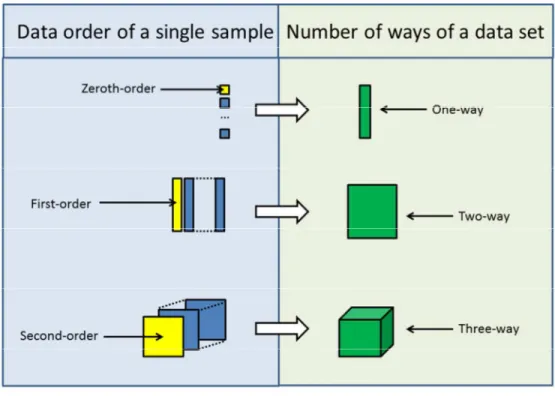
(8) Submitted to Chemical Reviews. 1 2 3 4 5 6 7 8 9 10 11 12 13 14 15 16 17 18 19 20 21 22 23 24 25 26 27 28 29 30 31 32 33 34 35 36 37 38 39 40 41 42 43 44 45 46 47 48 49 50 51 52 53 54 55 56 57 58 59 60. equation, and (2) the expression 'uncalibrated' may be confused with 'unexpected' (see below), which implies a different concept. The constituents present in unknown test samples, but not in the calibration or validation samples, are called 'unexpected'. Additional overlapping responses from the sample background may also be unexpected if not present during calibration. Unexpected constituents are also called potential interfering agents, with emphasis in 'potential', because in multi-way calibration their presence in a test sample may not lead to a systematic error in the analyte determination.43 In contrast, in univariate and first-order calibration, unexpected constituents usually produce an interference. Note, in the remainder of this review, the distinction of constituent, which is a real chemical compound present in a given sample, from component, which in general refers to a mathematical entity needed to model a data array, which may or may not directly represent the behavior of a specific chemical constituent.. 2.2. Data arrays For a consistent nomenclature of different data types, the concept of 'order' can be employed, as is widely done in analytical chemistry studies.20 The order is a tensorial property of data measured for a single sample: scalars are zeroth-order tensors, and thus univariate calibration is also known as zeroth-order calibration. If spectra are measured (or other vectors per sample), the calibration becomes first-order (and multivariate instead of univariate). Increasing the number of data modes per sample leads to correspondingly complex data arrays, which give rise to higher order multivariate calibration (Figure 1). The order is also linked to the popular expression 'second-order advantage', which is common among analytical chemists. The second-order –8– ACS Paragon Plus Environment. Page 8 of 87.

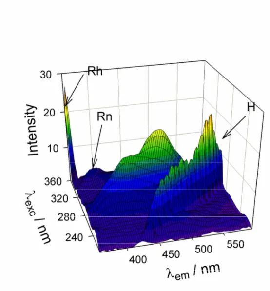
(9) Page 9 of 87. 1 2 3 4 5 6 7 8 9 10 11 12 13 14 15 16 17 18 19 20 21 22 23 24 25 26 27 28 29 30 31 32 33 34 35 36 37 38 39 40 41 42 43 44 45 46 47 48 49 50 51 52 53 54 55 56 57 58 59 60. Submitted to Chemical Reviews. advantage refers to the possibility of quantitating an analyte in a mixture with potentially interfering constituents, even when calibrating with pure analyte standards. It is not restricted to second-order data, but to all data of at least second-order.32 Interesting experimental applications in which this advantage has been exploited for a variety of samples can be found in recent reviews.22-31 An alternative nomenclature is based on the number of ways, which is equivalent to the number of modes of a data array for a group of samples.32 Thus univariate and one-way calibration are synonymous, as are first-order and two-way calibration, second-order and threeway calibration, etc. Three-way systems and beyond are also known as multi-way. Figure 1 visually summarizes the data array nomenclatures up to three-way (second-order). Popular examples of second-order data are excitation-emission fluorescence landscapes (Figure 2), which can be visually represented by plotting the fluorescence intensity as a function of excitation and emission wavelengths. When fluorescence excitation-emission matrix data (EEM data) are stacked together forming a three-way array (as in Figure 1), the latter object has three different modes: (1) the sample mode, (2) the excitation wavelength mode, and (3) the emission wavelength mode. The latter two will be referred as the instrumental data modes of the three-way data. Another popular form of second-order data is a chromatographic-spectral matrix, such as those collected on a liquid chromatograph with diode array detection (LC-DAD data) or fast-scanning fluorescence detection (LC-FSFD), or on a gas chromatograph with mass spectrometric detection (GC-MS data). Figure 3 shows a typical LC-FSFD landscape. Data matrices of this type can also be arranged into a three-way array whose modes are: (1) the sample mode, (2) the elution time mode, and (3) the spectral mode. Other three-way (second-order) data types are possible, as has been recently reviewed,22-26 but the number of works devoted to them are considerably smaller than for EEM or LC-spectral data. –9– ACS Paragon Plus Environment.

(10) Submitted to Chemical Reviews. 1 2 3 4 5 6 7 8 9 10 11 12 13 14 15 16 17 18 19 20 21 22 23 24 25 26 27 28 29 30 31 32 33 34 35 36 37 38 39 40 41 42 43 44 45 46 47 48 49 50 51 52 53 54 55 56 57 58 59 60. Page 10 of 87. Third-order data and beyond can easily be seen as extensions of the objects shown in Figure 1. Two usual manners in which they can be collected are: (1) measuring EEM while they evolve as a function of reaction time,44 or (2) acquiring two-dimensional chromatographic data (either LC-LC or GC-GC) with spectral (DAD or MS) detection.45,46 In all of these cases, three instrumental modes occur for each sample (excitation wavelength, emission wavelength and reaction time in one case, and first column elution time, second column elution time and spectra in the second), while the sample mode is the remaining one for a four-way array obtained by joining data for a group of samples.. 3. DATA PROPERTIES, MODELS AND ALGORITHMS 3.1. Univariate and first-order data Univariate calibration is well-known as the cornerstone of classical single-constituent calibration in analytical chemistry. Details can be found in IUPAC official protocols.9 The origins of first-order multivariate calibration date back to 1960s. Today it is established as a robust and reliable methodology for the analysis of industrial materials, with a paradigmatic example of the marriage between near infrared spectroscopy and partial leastsquares regression as a successful combination of instrumental and chemometric techniques.15 PLS is today the de facto standard for most first-order applications. Excellent reviews and books exist on the matter.12-14 Multi-way calibration is relatively new in this regard: the first work describing a secondorder calibration was published in 1978,47 reporting the determination of polycyclic aromatic hydrocarbons in the presence of potential interfering agents. Then an impasse of ca. 15 years elapsed, until the subject was revived in the mid 1990's.39 Although the number of multi-way – 10 – ACS Paragon Plus Environment.

(11) Page 11 of 87. 1 2 3 4 5 6 7 8 9 10 11 12 13 14 15 16 17 18 19 20 21 22 23 24 25 26 27 28 29 30 31 32 33 34 35 36 37 38 39 40 41 42 43 44 45 46 47 48 49 50 51 52 53 54 55 56 57 58 59 60. Submitted to Chemical Reviews. applications is exponentially growing, the methodology is still relatively unknown to the average analytical chemist. In contrast to univariate and first-order multivariate calibration, several multiway algorithms compete with success in the multi-way terrain. Their application fields overlap to some extent, and this may make the selection of a specific data processing algorithm a complex task. Therefore, information is provided in the next sections on the different types of multi-way data the analyst may find, and their relationship with the underlying model of various data processing algorithms.. 3.2. Multi-way data It is advisable to have some insight into the properties of the measured multi-way data, referring to an underlying physical model which the data are suspected to follow. Knowledge of the model allows one to select a specific data processing tool, which in turn significantly affects the achieved figures of merit. This is another peculiar feature of multi-way calibration: the algorithmspecificity of these figures. The simplest array in this regard is represented by second-order data measured for a single sample, which is also the basic ingredient of a three-way array. Two of the most popular experimental matrix data types, i.e., EEM and LC-spectral data, usually display a mathematical property called bilinearity. Assume an excitation-emission fluorescence data matrix X has been measured by scanning J different emission wavelengths and K different excitation wavelengths, or an LC-DAD matrix has been collected, consisting of J spectra measured at K elution times. In both cases, the data can be arranged into a data table or matrix with J rows and K columns, i.e., of size J×K. If there are N responsive constituents in the sample, a generic element xij of these data matrices can be written as: – 11 – ACS Paragon Plus Environment.

(12) Submitted to Chemical Reviews. 1 2 3 4 5 6 7 8 9 10 11 12 13 14 15 16 17 18 19 20 21 22 23 24 25 26 27 28 29 30 31 32 33 34 35 36 37 38 39 40 41 42 43 44 45 46 47 48 49 50 51 52 53 54 55 56 57 58 59 60. Page 12 of 87. N. xij =. ∑b. c. (1). jn kn. n =1. where bjn and ckn define the specific properties at instrumental channels j and k for constituent n. An error term should be added to the right hand side of eq (1) for completeness; it was omitted in this paper in all pertinent expressions for clarity. The meaning of 'instrumental channel' depends on the experimental setup, i.e., excitation/emission/absorption wavelength, elution time, mass/charge ratio, etc. Notice that signal additivity of the N constituents is assumed in eq (1), as is usual in the above described experimental situations. Figure 4 illustrates the obtainment of a matrix element from the individual profiles. Equation (1) is equivalent to: X = b1c1T + … bN cNT = B CT. (2). where the superscript 'T' indicates transposition, and bn and cn are vectors describing the profiles for constituent n in both data modes (Figure 4). Hence X is the sum of N terms, each of them linear in bn and cn, which are called bilinear components. For these reasons X is known as a bilinear matrix. To be precise, any data matrix can be expressed as a product of two matrices, however if the number of bilinear components required to adequately model a data matrix to a reasonable degree (the mathematical rank) is small and ideally equal to the number of responsive chemical constituents, then the matrix is said to be bilinear, although a proper nomenclature would be low-rank bilinear. When a data matrix for a mixture of a few constituents cannot be expressed as a sum of a few bilinear terms, it is called non-bilinear. This occurs, for example, for two-dimensional mass spectrometry (MS-MS),48 two-dimensional nuclear magnetic resonance correlated spectroscopy (2D NMR COSY),49 and total synchronous fluorescence (TSF) spectroscopy,50 because a spectrum in one mode depends on its position in the second mode. In. – 12 – ACS Paragon Plus Environment.

(13) Page 13 of 87. 1 2 3 4 5 6 7 8 9 10 11 12 13 14 15 16 17 18 19 20 21 22 23 24 25 26 27 28 29 30 31 32 33 34 35 36 37 38 39 40 41 42 43 44 45 46 47 48 49 50 51 52 53 54 55 56 57 58 59 60. Submitted to Chemical Reviews. general, bilinearity is lost when the phenomena occurring in the two instrumental modes are mutually dependent. For the simplest multi-way data, i.e., a three-way array, a particularly appealing property is the trilinearity, which naturally follows as the next step after bilinearity. As noted above, a three-way data array is trilinear (more precisely low-rank trilinear) if it can be expressed as a sum of a few trilinear components when the mixture contains a few constituents. Since EEM data are prime examples of trilinearity, they will be used as example. Assume a number of excitationemission fluorescence data matrices (I) has been measured. They can be stacked in the sample mode, creating a three-way array X, of size I×J×K, whose generic element can be designated as xijk. If the samples are mixtures of N fluorescent constituents, a specific signal xijk at sample i, emission wavelength j and excitation wavelength k can be written as: N. xijk =. ∑a. in. b jn ckn. (3). n =1. where ain is proportional to the concentration of constituent n in sample i, bjn to the emission quantum yield at wavelength j, and ckn to the absorption coefficient at excitation wavelength k. Equation (3) is analogous to the one relating the fluorescence emission intensity to the usual chemical and instrumental parameters involved in this phenomenon,51 except for a scaling factor and a change in symbols. It is customary to collect all ain values into a vector an, bjn into a vector bn, and ckn into a vector cn. The latter two vectors are usually normalized to unit length. It is perhaps not directly apparent in eq (3), but trilinearity demands that: (1) individual data matrices are bilinear, i.e., b and c profiles do not depend on each other, and (2) b and c profiles do not depend on the sample index i, i.e., there should be unique b and c vectors describing the behaviour of each constituent in both instrumental modes in all samples. These. – 13 – ACS Paragon Plus Environment.

(14) Submitted to Chemical Reviews. 1 2 3 4 5 6 7 8 9 10 11 12 13 14 15 16 17 18 19 20 21 22 23 24 25 26 27 28 29 30 31 32 33 34 35 36 37 38 39 40 41 42 43 44 45 46 47 48 49 50 51 52 53 54 55 56 57 58 59 60. Page 14 of 87. conditions are usually met by EEM spectroscopy, which provides primary examples of trilinear three-way data (except for the diffraction grating harmonics, which can generally be corrected). In the case of data stemming from chromatography with spectral detection, the data matrices are individually bilinear; however, small changes in elution profiles for a given constituent from sample to sample usually occur. Hence a three-way array composed of these latter data matrices will not be, in general, trilinear. They would be if elution profiles were exactly reproducible from sample to sample. For this reason, the elution time mode is a potentially trilinearity-breaking mode.52 Three-way data having a single trilinearity-breaking mode can be conveniently analyzed if the three-way array is unfolded along the elution time mode, i.e., if it is converted into a data matrix having all individual sample data matrices adjacent to each other in the direction of the elution time (Figure 5). The latter data matrix is called augmented, because it can be viewed as being built from the individual matrices by the process of augmentation (it can also be viewed as arising from the unfolding process which starts from the three-way array, see Figure 5). Since the individual data matrices are bilinear, an important property of a chromatographic-spectral matrix augmented in the time direction (Xaug) is that it is also bilinear, i.e., it can be formulated as: N. xaug,pk =. ∑b. aug, pn. ckn. (4). n =1. with the index p running from 1 to IJ, because the size of the augmented matrix is IJ×K (I = No. of samples, J = No. of elution times, K = No. of wavelengths). In eq (4), the spectral profile cn (also called the non-augmented profile) is unique for each constituent and common to all samples, whereas baug,n is the augmented time profile in the augmented elution time mode, and is composed of I successive time sub-profiles with J times each.. – 14 – ACS Paragon Plus Environment.

(15) Page 15 of 87. 1 2 3 4 5 6 7 8 9 10 11 12 13 14 15 16 17 18 19 20 21 22 23 24 25 26 27 28 29 30 31 32 33 34 35 36 37 38 39 40 41 42 43 44 45 46 47 48 49 50 51 52 53 54 55 56 57 58 59 60. Submitted to Chemical Reviews. Table 1. Classification of second- and third-order data, and models/algorithms which can be applied to analyze them. Three-way (second-order) data Data type. Example. Suitable algorithm. Trilinear. EEM. PARAFACa. Non-trilinear with one breaking mode. LC-DAD. MCR-ALS. LC-FSFD GC-MS Other non-trilinear. Two trilinearity breaking modes. EEM with inner filter. PLS/RBL. Non-bilinear individual matrices. MS-MS. PLS/RBLb. 2. D NMR COSY. TSF Four-way (third-order) data Quadrilinear. EEM-time. PARAFACa. Non-quadrilinear with two quadrilinearity breaking modes. LC-LC-DAD. MCR-ALS. Other non-quadrilinear. –. GC-GC-MS –. a. Additional multi-linear decomposition variants are also possible.55-58. b. PLS/RBL has only been applied to TSF data.50. Several other instrumental second-order data exist, although they are not employed as often for analytical calibration purposes. Among these other data, two additional non-trilinear data types may be found, for which: (1) individual data matrices are non-bilinear (see above for examples), and (2) individual data matrices have two trilinearity breaking modes, because both instrumental profiles vary from sample to sample, and augmentation into a bilinear matrix is not – 15 – ACS Paragon Plus Environment.

(16) Submitted to Chemical Reviews. 1 2 3 4 5 6 7 8 9 10 11 12 13 14 15 16 17 18 19 20 21 22 23 24 25 26 27 28 29 30 31 32 33 34 35 36 37 38 39 40 41 42 43 44 45 46 47 48 49 50 51 52 53 54 55 56 57 58 59 60. Page 16 of 87. possible, such as EEM fluorescence data in the presence of inner filter effects in both the excitation and emission modes.53 As a consequence, it is sensible to classify three-way data in: (1) trilinear, (2) non-trilinear with a single trilinearity-breaking mode and unfoldable to a bilinear augmented matrix, and (3) other non-trilinear, as summarized in Table 1 including pertinent examples. It is interesting to note that ca. 90% of the published multi-way calibration works describe data belonging to the first two categories, distributed in almost equal shares. In going to more data orders, a similar classification scheme is possible. In general, multiway data can be arranged into a multi-way array, which is multi-linear if its elements obey an equation similar to eq (3); for four-way (third-order) data, for example: N. xijkl =. ∑a. in. b jn ckn d ln. (5). n =1. where the extra factor in comparison with eq (3) corresponds to the profile in the additional data mode. Multi-linearity requires profiles in all data modes which are independent of each other and independent of sample. A typical example involves the measurement of the time evolution of EEM data while following the kinetics of a reaction.44 If there are multi-linearity breaking instrumental modes in multi-way arrays, unfolding the array into a bilinear augmented matrix may be possible. This is typical of third-order chromatographic data such as LC-LC-DAD and GC-GC-MS, which display two potentially quadrilinearity-breaking modes (the two elution time modes). In this case, it is wise to unfold the four-way array into an augmented data matrix whose modes are: (1) the spectral mode (either DAD or MS), which is the non-augmented mode, and (2) a concatenation of both elution time modes into a single one, which is the augmented mode.45,46 Additional four- and higher-way data types can be envisaged beyond those quoted in Table 1, as the different data modes might in. – 16 – ACS Paragon Plus Environment.

(17) Page 17 of 87. 1 2 3 4 5 6 7 8 9 10 11 12 13 14 15 16 17 18 19 20 21 22 23 24 25 26 27 28 29 30 31 32 33 34 35 36 37 38 39 40 41 42 43 44 45 46 47 48 49 50 51 52 53 54 55 56 57 58 59 60. Submitted to Chemical Reviews. principle be multi-linearity breaking, and/or mutually interacting with each other. However, the number of experimental developments in this regard is still small.. 3.3. Multi-way models and algorithms There are many available algorithms for analytical calibration with multi-way data. Priority is given to those allowing for multiple calibration samples, because this leads to more robust and statistically efficient analytical results.35 The most employed algorithms in this regard can be appropriately classified into three main groups according to a simple connection between their underlying models and the different data categories discussed in the previous section: (1) a multilinear model, (2) a bilinear model for an augmented matrix, and (3) a flexible latent-variable model. Group (1) includes parallel factor analysis (PARAFAC)54 and some variants,55-58 group (2) multivariate curve resolution coupled to alternating least-squares (MCR-ALS)59 particularly in the so-called extended version,60 and group (3) unfolded and multi-way partial least-squares (U-PLS and N-PLS).61,62 Additional, less employed algorithms for multi-way calibration are worth mentioning, such as multi-linear least-squares (MLLS),63,64 a less flexible version of the PLS methodologies, and generalized rank annihilation (GRAM),65 direct trilinear decomposition (DTLD),66 and non-bilinear rank annihilation (NBRA).49 The latter three algorithms are based on calibration with a single standard (either real or virtual). A fundamental difference between PARAFAC and MCR-ALS is that the former often leads to unique solutions,54 whereas MCR-ALS needs to apply a series of constraints (all of them based on natural physico-chemical assumptions) in order to reach a chemically reasonable solution.59,60 The uniqueness property of PARAFAC regarding the decomposition of a multi-way array into a small number of trilinear components has a direct consequence in the achievement of – 17 – ACS Paragon Plus Environment.

(18) Submitted to Chemical Reviews. 1 2 3 4 5 6 7 8 9 10 11 12 13 14 15 16 17 18 19 20 21 22 23 24 25 26 27 28 29 30 31 32 33 34 35 36 37 38 39 40 41 42 43 44 45 46 47 48 49 50 51 52 53 54 55 56 57 58 59 60. Page 18 of 87. the second-order advantage, because it leads to pure signals and relative concentrations of all sample constituents, including the analyte of interest. It may be noticed that both PARAFAC and MCR-ALS achieve the second-order advantage by simultaneously processing multiple calibration samples and unknowns, because their internal algorithmic models are able to decompose the contribution of the potential interfering agents and the analytes to the total signal. However, in the case of the PLS-based methodologies, the achievement of the second-order advantage is a post-calibration activity: the test sample is subjected to a procedure called residual multi-linearization (RML, including bi-, tri- and quadrilinearization, i.e., RBL,63,67,68 RTL64 and RQL69), which separates the portion of the signal which can be explained by calibration from the contribution of the potential interfering agents. This gives rise to the hybrid methodologies PLS/RML. Details on the operation of all these algorithms can be found in the Supporting Information and in relevant reviews.22-26 At the risk of some oversimplification, Table 1 shows a correspondence between data properties and algorithms. Multi-linear algorithms such as PARAFAC are the natural choice for multi-linear data, extended MCR-ALS is based on an augmented bilinear matrix and hence it is also natural to select it when the data are non-multi-linear but follows the augmented bilinear model, and finally latent-variable PLS/RML methodologies display a flexibility which should made them the algorithms of choice for other non-multilinear data. However, the application fields of these algorithms considerably overlap because of several facts: (1) MCR-ALS and PLS/RML can be applied to multi-linear data, (2) chromatographic profiles can in certain cases be aligned or synchronized,70 so that their shapes and positions in the elution time axis become common to all samples, restoring multi-linearity, and (3) PARAFAC variants have been developed (i.e., PARAFAC2)71 for coping with varying chromatographic profiles from sample to sample. These three events may make model and algorithm selection a more complex task for the – 18 – ACS Paragon Plus Environment.

(19) Page 19 of 87. 1 2 3 4 5 6 7 8 9 10 11 12 13 14 15 16 17 18 19 20 21 22 23 24 25 26 27 28 29 30 31 32 33 34 35 36 37 38 39 40 41 42 43 44 45 46 47 48 49 50 51 52 53 54 55 56 57 58 59 60. Submitted to Chemical Reviews. average chemist. However, it is likely that future developments will take into account sensitivity considerations as a helpful decision-making tool in this regard.. 4. SENSITIVITY EXPRESSIONS BASED ON SIGNAL OR NET SIGNAL CHANGES 4.1. Univariate calibration In univariate calibration, prediction of the analyte concentration (y) in a test sample from its signal (x) proceeds through the known expression:9 y = (x – n0) / m0. (6). where m0 and n0 are the slope and intercept, respectively, of the zeroth-order linear calibration graph. The slope m0 is the sensitivity, since it measures the change in signal for a unit change in concentration.9. 4.2. First-order calibration The concept of net analyte signal has been useful in assessing the sensitivity in first-order calibration, by extending the univariate definition to the change in NAS for a unit change in analyte concentration.17 In order to fully understand the NAS concept and its consequences, it is highly useful to consider the simplest possible example, i.e., a binary mixture where two constituents occur, with the vector signal (e.g., a spectrum) for a test sample measured at a number of sensors and given by: x = y1 s1 + y2 s2. (7). where y1 and y2 are the constituent concentrations and s1 and s2 the pure constituent profiles at unit concentration. By employing eq (7) it is implicitly assumed that: (1) the studied signal is – 19 – ACS Paragon Plus Environment.

(20) Submitted to Chemical Reviews. 1 2 3 4 5 6 7 8 9 10 11 12 13 14 15 16 17 18 19 20 21 22 23 24 25 26 27 28 29 30 31 32 33 34 35 36 37 38 39 40 41 42 43 44 45 46 47 48 49 50 51 52 53 54 55 56 57 58 59 60. Page 20 of 87. additive, i.e., the total signal is the sum of the individual contributions from both sample constituents, and (2) the constituent signals are proportional to their concentrations, meaning that Beer's law (or its analogues) apply. Figure 6A shows two typical pure constituent spectra at unit concentration, and Figure 6B the spectrum for a mixture at equal analyte concentrations, including the individual contributions of each constituent to the mixture spectrum. Focusing on analyte 1 as the compound of interest, the contribution from constituent 2 can be removed from eq (7) by left-multiplying both sides by an orthogonal projection matrix [I – s2 (s2T s2)–1 s2T], where I is an appropriately dimensioned unit matrix (orthogonal means in this context 'perpendicular' to a generalized plane in the multivariate space). Usually the result of [(s2T s2)–1 s2T] is designated as s2+, with the superscript '+' implying the generalized inverse operation. Notice that knowledge of s1 and s2 is assumed, which is only possible in the context of first-order methodologies such as classical least-squares (CLS) analysis, where the pure spectra are either supplied to the model from separate measurements on pure constituents, or are adequately retrieved by analysis of mixtures of pure constituents. Removal of the contribution of the concomitant No. 2 in the mixture by orthogonal projection is possible because (I – s2 s2+)×s2 = s2 – s2 = 0. Equation (7) thus leads to: (I – s2 s2+) x = y1 (I – s2 s2+) s1. (8). By performing this rather smart operation, a two-constituent problem has become a virtual single-constituent problem. Indeed, the left hand side of the latter equation defines the net analyte signal for constituent 1 in the mixture ( x1* ), as being proportional to its NAS at unit concentration ( s1* ), the proportionality constant being the analyte concentration y1:. x1* = y1s1*. (9). – 20 – ACS Paragon Plus Environment.

(21) Page 21 of 87. 1 2 3 4 5 6 7 8 9 10 11 12 13 14 15 16 17 18 19 20 21 22 23 24 25 26 27 28 29 30 31 32 33 34 35 36 37 38 39 40 41 42 43 44 45 46 47 48 49 50 51 52 53 54 55 56 57 58 59 60. Submitted to Chemical Reviews. In sum, the NAS in the mixture and the NAS at unit concentration, both specific to analyte 1, are defined by projecting, orthogonal to the space spanned by the remaining sample constituent 2 (s2), the sample signal x and the pure analyte signal s1 respectively. Figure 7 pictorially illustrates the process of projecting the x vector orthogonally to the space spanned by constituent 2 (the plane in this figure is only intended as a graphical representation of the multidimensional surface corresponding to the vector s2). The relevant result to be gathered from eq (9) is that the NAS vector x1* is parallel to the NAS at unit concentration s1* . Figure 8A shows these NAS vectors, which are seen to be rather abstract linear combinations of true profiles and thus lacking intuitive interpretation. The real usefulness of the NAS lies in the fact that a plot of the length of the NAS vector (|| x1* ||, also called the scalar NAS, and given as the square root of the sum of the squared elements of the x1* vector) as a function of analyte concentration is linear, the slope being the length of the NAS vector at unit concentration (|| s1* ||) (Figure 8B).72-74 This immediately leads to an intuitive definition of sensitivity for analyte 1 as follows (see Appendix A-1 for details):. [ (. ) ]. T SEN1 = || x1* || / y1 = || s1* || = s1 I − s 2 s 2+ s1. 1/ 2. (10). In conclusion, if both vectorial signals at unit concentration for the pure constituents of a mixture are known, or can be estimated from the analysis of mixtures of pure constituents, simple matrix manipulation allows one to precisely define the sensitivity towards a given constituent. A useful relationship between the sensitivity based on this NAS approach and the complete matrix of pure constituent signals can be found by invoking the theory of block pseudo-inverse operations.75 As discussed in Appendix A-1, eq (10) can be generalized to the nth constituent of interest in a multi-constituent sample in different forms. One useful form is expressed as a function of the pure profiles for all constituents, ubiquitous in CLS studies: – 21 – ACS Paragon Plus Environment.

(22) Submitted to Chemical Reviews. 1 2 3 4 5 6 7 8 9 10 11 12 13 14 15 16 17 18 19 20 21 22 23 24 25 26 27 28 29 30 31 32 33 34 35 36 37 38 39 40 41 42 43 44 45 46 47 48 49 50 51 52 53 54 55 56 57 58 59 60. [. (. SENn = δ Tn S TCLSS CLS. ). −1. ]. Page 22 of 87. −1 / 2. δn. (11). where δn is an N×1 vector selecting the analyte of interest (see Appendix A-1), and the matrix SCLS contains N columns, each with the pure constituent profile sn for the nth constituent. Another useful generalization of the multivariate first-order sensitivity can be developed in terms of the so-called vector of regression coefficients, which is specific for a given analyte in a mixture (β βCLS,n). This vector provides the analyte concentration from the predictive equation:. yn = βTCLS,n x. (12). As a function of this vector, the sensitivity can be expressed as:. (. T. SENn = β CLS,n βCLS,n. ). −1/ 2. (13). Equation (13) provides a useful link to first-order algorithms which do not rely on the estimation of pure constituent profiles. The latter ones are the so-called inverse models, such as inverse least-squares (ILS), principal component regression (PCR) and PLS.37,76 In contrast to the direct approach of the classical Beer's law, inverse calibration models relate concentrations to signals, i.e.:. yn = β Tn x. (14). Inverse algorithms are able to provide a vector of regression coefficients βn from a suitable set of calibration mixtures, and thus the analogue of eq (13) is a useful means of estimating the sensitivity for these methodologies. Appendix A-1 shows how eq (11) can be adapted to make it compatible with those for latent based methodologies, by replacement of δn and SCLS with appropriate latent-variable mathematical objects. In this way, sensitivity expressions for both direct and inverse calibration first-order methodologies can be brought into a common form. – 22 – ACS Paragon Plus Environment.

(23) Page 23 of 87. 1 2 3 4 5 6 7 8 9 10 11 12 13 14 15 16 17 18 19 20 21 22 23 24 25 26 27 28 29 30 31 32 33 34 35 36 37 38 39 40 41 42 43 44 45 46 47 48 49 50 51 52 53 54 55 56 57 58 59 60. Submitted to Chemical Reviews. 4.3. Multi-way (higher-order) calibration One approach for estimating the SENn parameter in three-way (second-order) calibration is the calculation of the net analyte signal inspired in the useful first-order NAS philosophy, removing the contribution of constituents other than the analyte of interest using orthogonal projection matrices. One intriguing aspect of this multi-way NAS approach is the fact that, in principle, these projections can be carried out in different ways, leading to competing NAS definitions.35 A typical matrix signal (X) defined in two different instrumental modes for a simple binary mixture can be written as: X = y1 M1 + y2 M2. (15). where M1 and M2 are matrix signals at unit concentration for each analyte, and, as before, signal additivity and signal-concentration linearity are assumed. If the signals are bilinear, and the profiles in both data modes are designated as b and c, the expression for X would be: X = y1 b1 c1T + y2 b2 c2T. (16). where b1 and b2 the pure constituent profiles in the first data mode, and c1 and c2 those in the second data mode. For EEM data, b and c describe excitation and emission spectral profiles, while in LC-spectral data, they correspond to elution time and spectral profiles respectively. Following the NAS approach, the contributing matrix signal for the constituent No. 2 may be removed from eq (16) by these simultaneous operations: left-multiplication with a projection matrix orthogonal to b2, and right-multiplication with an analogous matrix orthogonal to c2. Without going into the specific details, the relevant outcome is that this line of reasoning leads to one particular sensitivity expression known as HCD (acronym follows authors initials),33 which is valid in a certain calibration scenario. Table 2 shows the specific expression and applicability.35 Figure 9 shows the graphical result for a typical binary mixture where the constituents are described in both data modes by Gaussian-shaped profiles such as the pure – 23 – ACS Paragon Plus Environment.

(24) Submitted to Chemical Reviews. 1 2 3 4 5 6 7 8 9 10 11 12 13 14 15 16 17 18 19 20 21 22 23 24 25 26 27 28 29 30 31 32 33 34 35 36 37 38 39 40 41 42 43 44 45 46 47 48 49 50 51 52 53 54 55 56 57 58 59 60. Page 24 of 87. spectra shown in Figure 4. As was the case with the first-order NAS counterpart, the secondorder NAS landscape for the HCD definition does not lead to an obvious physical interpretation.. Table 2. Different three-way (second-order) sensitivity definitions based on extensions of the NAS concept. Expressiona. Comments. Ref.. SENn = mn {[(BT B) –1]nn [(CT C)–1]nn }–1/2. HCD sensitivity, valid for one calibrated constituent in the presence of unexpected constituents. 33. SENn = mn {[(BT B) * (CT C)]–1}nn–1/2. MKL sensitivity, valid in the absence of unexpected constituents. 34. SENn = mn {[(BexpT (I – Bunx Bunx+) Bexp) *. FO sensitivity, valid for any number of calibrated constituents in the presence of unexpected constituents. 35. (CexpT (I – Cunx Cunx+) Cexp)]–1}nn–1/2 a. The symbol '*' is the Hadamard matrix product, and the subscript 'nn' indicates the (n,n) diagonal element of a matrix. The parameter mn is the total signal for the analyte of interest at unit concentration. The matrices B and C collect the loadings (profiles for the sample constituents in both data modes, normalized to unit length), with the subscripts 'exp' and 'unx' in the FO expression indicating expected and unexpected respectively.. There is an alternative approach, which involves first unfolding the matrix X into a vector, and then removing the contribution of constituent 2 with a single removing matrix, orthogonal to the unfolded space spanned by constituent 2. This unfolded space is formally represented by the so-called Kronecker product (c2⊗b2) = [c21 b2 | c22 b2 | ... ].77 This approach leads to a different second-order sensitivity definition, the MKL sensitivity (acronym follows authors initials),34 valid in a different calibration situation in comparison with the HCD sensitivity. Table 2 provides the corresponding information. Notice that the original works on HCD and MKL sensitivity did – 24 – ACS Paragon Plus Environment.

(25) Page 25 of 87. 1 2 3 4 5 6 7 8 9 10 11 12 13 14 15 16 17 18 19 20 21 22 23 24 25 26 27 28 29 30 31 32 33 34 35 36 37 38 39 40 41 42 43 44 45 46 47 48 49 50 51 52 53 54 55 56 57 58 59 60. Submitted to Chemical Reviews. not employ NAS arguments for their derivation, but the results are identical to those provided by the above NAS-inspired procedures.35 Figure 9 shows the plot of the MKL NAS surface: this sensitivity is higher than the HCD one (the vertical scales of Figure 9 are arbitrary, but the numerical limits for the intensity axes are identical). From Table 2, this appears to be the expected outcome from two radically different calibration situations: (1) both constituents are calibrated (MKL) and (2) one is calibrated and the second one is a potential interfering agent (HCD), which decreases the sensitivity. Both HCD and MKL equations were condensed into the more general FO definition (acronym follows authors initials),35 conceived to take into account all possible calibration situations, including cases not covered by the former two expressions (Table 2). The derivation required a complicated series of steps, which combined removal of other sample constituents, partly in matrix form and partly in unfolded form. This multiplicity of definitions and procedures is puzzling and lacks the elegance of the first-order NAS-based sensitivity counterpart. More importantly, however, the approach could not be straightforwardly extended to four-way (thirdorder) calibration, where it is apparent that even more alternative NAS definitions may exist.38 This situation prompted the finding of an alternative solution to the estimation of the multi-way sensitivity.. 5. SENSITIVITY EXPRESSIONS BASED ON UNCERTAINTY PROPAGATION 5.1. The general sensitivity expression An alternative and useful operative definition of sensitivity can be given in terms of uncertainty propagation: the sensitivity parameter SENn is considered to measure the degree of output noise – 25 – ACS Paragon Plus Environment.

(26) Submitted to Chemical Reviews. 1 2 3 4 5 6 7 8 9 10 11 12 13 14 15 16 17 18 19 20 21 22 23 24 25 26 27 28 29 30 31 32 33 34 35 36 37 38 39 40 41 42 43 44 45 46 47 48 49 50 51 52 53 54 55 56 57 58 59 60. Page 26 of 87. from a system for a given input noise.78,79 More sensitivity is achieved if low output noise is obtained for a given input noise (Figure 10). It then makes perfect sense to define the SENn parameter as the ratio of input to output noise: SENn = σx / σy. (17). where σx and σy are the uncertainties in signal and concentration respectively. This uncertainty propagation approach assumes that the input noise is independent and identically distributed, and employs a small, perturbing noise value to interrogate how the latter is propagated to prediction. However, it does not imply specific assumptions regarding the properties of the real experimental noise. When calibration is precise, the main source of uncertainty in the predicted concentration is the one stemming from the test sample signals, and the ratio of these uncertainties is a good measure of the SENn. Therefore the box labeled 'Calibration model' in Figure 10 refers to a precisely defined model in terms of a set of calibration samples with known reference concentrations, all of them carrying negligible uncertainty in both signals and concentrations. The scheme shown in Figure 10 can be mirrored by a Monte Carlo additive noise simulation for estimating sensitivities for any calibration model, whether univariate, multivariate or multi-way, as has been recently done.40-42 This allowed operational values for the sensitivity in different calibration scenarios to be obtained, although they do not provide a closed-form sensitivity equation, which would be far more useful in this regard. Recently, several expressions were derived using the concept of uncertainty propagation from a noisy test sample signal to the concentration predicted by a noiseless calibration model.40-42 The developed equations allowed to estimate the sensitivity in most of the relevant multi-way calibration models, including PARAFAC, MCR-ALS and PLS/RML, with results. – 26 – ACS Paragon Plus Environment.

(27) Page 27 of 87. 1 2 3 4 5 6 7 8 9 10 11 12 13 14 15 16 17 18 19 20 21 22 23 24 25 26 27 28 29 30 31 32 33 34 35 36 37 38 39 40 41 42 43 44 45 46 47 48 49 50 51 52 53 54 55 56 57 58 59 60. Submitted to Chemical Reviews. which are: (1) compatible with the second-order HCD, MKL and FO (when they apply, see Table 2), (2) in agreement with Monte Carlo additive noise simulations for data of various orders, and (3) extendable to data with increasing number of ways. From this body of work, it is now possible to write an expression for casting all sensitivity equations into a single unified scheme, covering from zeroth-order (univariate calibration) to calibration models based on data of any order and ways. The main result is appropriately condensed into the following expression:. { [. (. ). SENn = g Tn Z Texp I − Z unx Z +unx Z exp. ]. −1. }. −1 / 2. gn. (18). The different factors appearing in eq (18) will be explained below in the context of each calibration scenario, but a qualitative description is appropriate at this point. Both the matrix Zexp (the subscript 'exp' stands for expected) and the analyte-specific vector gn correspond to the calibration phase. The matrix Zexp collects profiles (either in pure form or as linear combinations) for the expected constituents present in the calibration set, while gn adequately selects or combines the latter information, making it specific for the nth analyte of interest. The final factor in eq (18) is the matrix. (I−Z. unx. Z +unx ) , which is the mathematical manifestation of the second-. order advantage, and thus it only appears in higher-order (three-way and beyond) calibration methodologies. Its purpose is to correct the matrix of profiles for the expected constituents (Zexp) for the overlapping effect of the profiles for the unexpected constituents (hence the subscript 'unx') or potential interfering agents. Specifically, the matrix. (I−Z. unx. Z +unx ) depends on the. profiles for the unexpected constituents which may occur in a given test sample, and only appears when achieving the second-order advantage, because only in this case is such information available. The profiles for the unexpected constituents may be: (1) true constituent profiles (or approximations to them) provided, for example, by MCR-ALS, PARAFAC and all its multi– 27 – ACS Paragon Plus Environment.

(28) Submitted to Chemical Reviews. 1 2 3 4 5 6 7 8 9 10 11 12 13 14 15 16 17 18 19 20 21 22 23 24 25 26 27 28 29 30 31 32 33 34 35 36 37 38 39 40 41 42 43 44 45 46 47 48 49 50 51 52 53 54 55 56 57 58 59 60. Page 28 of 87. linear decomposition variants or (2) latent profiles (linear combinations or loadings) retrieved by RML. What is relevant is that. (I−Z. unx. Z +unx ) defines a projection orthogonal to the space. spanned by the unexpected constituents, because Zunx only contains information relative to the signals for the latter agents. Although the specific form of Zunx differs from the simple intuitive expectations based on the direct extension of the NAS concept from first- to higher-order, a germ of eq (18) can already be anticipated from inspection of the FO expression shown in Table 2, which is not based on uncertainty propagation principles. The fact that closed expressions for Zexp, gn and. (I−Z. unx. Z +unx ) can be written for all. calibration methodologies from zeroth-order to any order (see Table 3) implies that eq (18) is the most general expression available for estimating sensitivities. It is also worth noticing the properties of the multi-way sensitivity defined by eq (18): (1) it is analyte-specific, because the factor gn depends on the analyte of interest, (2) it is sample-specific, because the composition of each test sample is unique as regards the unexpected constituents, generating a unique Zunx matrix, and (3) it is algorithm-specific, because each data processing methodology provides a set. (. ). of specific Zexp, gn and I − Z unx Z +unx factors.. – 28 – ACS Paragon Plus Environment.

(29) Page 29 of 87. 1 2 3 4 5 6 7 8 9 10 11 12 13 14 15 16 17 18 19 20 21 22 23 24 25 26 27 28 29 30 31 32 33 34 35 36 37 38 39 40 41 42 43 44 45 46 47 48 49 50 51 52 53 54 55 56 57 58 59 60. Submitted to Chemical Reviews. Table 3. General sensitivity expression and detailed parameters for the various calibration methodologies applicable to data of increasing order.. { [. Model Univariate CLS. (. ). SENn = g Tn Z Texp I − Z unx Z +unx Z exp. General expression Order 0 1. gn 1 δn. Zexp m0 SCLS. Zunx – –. ILS. 1. ycal,n. Xcal. –. PCR. 1. vPCR,n. PPCR. –. PLS. 1. qPLS,n. WPLS. –. MCR-ALS. 2. δn. mn Cexp J 1/ 2. Cunx. PARAFAC. 2, 3, .... δn. See last column. See Table 4. U-PLS/RMLa. 2, 3, .... vUPLS,n. PUPLS. N-PLS/RMLa. 2, 3, .... vNPLS,n. See Table 4 See Table 4. ]. −1. }. −1 / 2. gn. Comments m0 = slope of univariate graph δn = Kronecker vector for analyte n SCLS = matrix of pure constituent profiles ycal,n = vector of calibration analyte concentrations Xcal = matrix of calibration signals vPCR,n = vector of latent PCR coefficients PPCR = matrix of PCR calibration loadings T q PLS,n = ( PPLS WPLS ) −1 v TPLS,n vPLS,n = vector of latent PLS coefficients WPLS = matrix of PLS calibration weights PPLS = matrix of PLS calibration loadings J = No. of sensors of each sub-matrix in augmented mode mn = slope of pseudo-univariate plot Cexp = profiles in non-augmented mode for expected constituents in calibration Cunx = profiles in non-augmented mode for unexpected constituents Second-order: Zexp = mn Cexp☼Bexp Third-order: Zexp = mn Dexp☼Cexp☼Bexp Fourth-order: Zexp = mn Eexp☼Dexp☼Cexp☼Bexp Bexp, Cexp, Dexp, and Eexp are loading matrices in the various data modes for the expected constituents in calibration PUPLS = matrix of U-PLS calibration loadings vUPLS,n = vector of latent PLS coefficients. WNPLS = matrix of N-PLS calibration weights Second-order:b WNPLS = WK☼WJ Third-order:b WNPLS = WL☼WK☼WJ Fourth-order:b WNPLS = WM☼WL☼WK☼WJ vNPLS,n = vector of latent N-PLS coefficients a RML = residual multi-linearization (includes RBL, RTL, RQL). b J, K, L and M identify the different data modes. WNPLS. – 29 – ACS Paragon Plus Environment.

(30) Submitted to Chemical Reviews. 1 2 3 4 5 6 7 8 9 10 11 12 13 14 15 16 17 18 19 20 21 22 23 24 25 26 27 28 29 30 31 32 33 34 35 36 37 38 39 40 41 42 43 44 45 46 47 48 49 50 51 52 53 54 55 56 57 58 59 60. Page 30 of 87. 5.2. Univariate calibration In the classical one-way (zeroth-order) or univariate calibration, the relevant parameters from the general eq (18) are scalars (Zunx does not exist, since no unexpected constituents are possible in this methodology), gn = 1 and Zexp = m0, leading to SENn = m0, the slope of the calibration graph. This agrees with the IUPAC definition, and of course with the simple and intuitive uncertainty analysis of eq (6): if calibration were precise, uncertainties in x will propagate to y through σy = m0–1 σx, and thus SENn will be equal to m0.. 5.3. First-order calibration In the first-order calibration world, the definitions of Zexp and gn depend on the specific data processing algorithm (Table 3). In any case, since no unexpected constituents should appear in. (. ). the test samples, Zunx does not exist and thus I − Z unx Z +unx = I. It is apparent that the general eq (18) gives eq (11) for CLS, and analogous expressions for ILS, PCR and PLS [see Appendix A-1, eqs (A-10)-(A-12)], in full agreement with the NAS-based sensitivity approach. Again, uncertainty propagation provides these results directly from the general predictive equation for analyte n: y n = β Tn x. (19). where βn is the vector of regression coefficient for any first-order methodology. If only x carries uncertainty, it follows that the uncertainty in concentration is given by:. (. σy = β Tn β n. ). 1/ 2. σx. (20). From this latter expression, SENn =. (β β ) T n. −1 / 2. n. immediately follows through the. uncertainty propagation approach, in agreement with eq (A-10) of Appendix A-1. This sensitivity – 30 – ACS Paragon Plus Environment.

(31) Page 31 of 87. 1 2 3 4 5 6 7 8 9 10 11 12 13 14 15 16 17 18 19 20 21 22 23 24 25 26 27 28 29 30 31 32 33 34 35 36 37 38 39 40 41 42 43 44 45 46 47 48 49 50 51 52 53 54 55 56 57 58 59 60. Submitted to Chemical Reviews. parameter is clearly analyte-specific but does not depend on the composition of the test sample, because the vector of regression coefficients stems from the processing of the calibration data only. One may argue that it is algorithm-specific, because different algorithms (CLS, ILS, PCR, PLS) will provide different regression vectors β n. However, algorithm-specificity explicitly refers to the wildly different Zunx matrices provided by multi-way algorithms, which may cause the sensitivity to markedly differ from one algorithm to the other.. 5.4. Multi-way (higher-order) calibration 5.4.1. Multi-linear algorithms Multi-linear algorithms such as PARAFAC54 and its variants based on the multi-linear model55-58 provide approximations to pure constituent profiles, whether they belong to the category of expected or unexpected. Each constituent is characterized by instrumental profiles describing their behavior in the different data modes. In the usual setting, these profile vectors are normalized to unit length, and thus the scaling factor with respect to analyte concentration is left to the slope (mn) of the pseudo-univariate prediction graph (the latter is a plot of the scores or relative concentrations of a given analyte vs. its nominal calibration concentrations). What is peculiar in the case of these multi-way algorithms achieving the second-order advantage is that they are able to provide profiles for the potentially interfering constituents in a given test sample. As a function of the relevant parameters for multi-linear multi-way calibration, the recently derived expression for the sensitivity in multi-linear models is:40 SENn = mn || nth row of [(I – Zunx Zunx+) Zexp]+ ||–1. – 31 – ACS Paragon Plus Environment. (21).

(32) Submitted to Chemical Reviews. 1 2 3 4 5 6 7 8 9 10 11 12 13 14 15 16 17 18 19 20 21 22 23 24 25 26 27 28 29 30 31 32 33 34 35 36 37 38 39 40 41 42 43 44 45 46 47 48 49 50 51 52 53 54 55 56 57 58 59 60. Page 32 of 87. The matrix Zexp is defined in Table 3 as a function of the loading matrices for second-, third- and fourth-order as in eqs. (22), (23) and (24) respectively, while Table 4 shows the specific forms of the Zunx matrix: Zexp = mn (Cexp☼Bexp). (22). Zexp = mn (Dexp☼Cexp☼Bexp). (23). Zexp = mn (Eexp☼Dexp☼Cexp☼Bexp). (24). In the latter expressions, the symbol '☼' indicates the Khathri-Rao product operator,75 also known as the column-wise Kronecker product, because for matrices A and B, the ith. column of A☼B follows from the ith. columns of A and B as ai⊗bi. Therefore, the columns of Zexp are proportional to the pure signals for each constituent in the calibration set, each unfolded into a vector and normalized to unit length.. Table 4. Content of the matrix representing the space spanned by the unexpected constituents in multi-way (higher-order) calibration. Order. Zunxa. 2. [ c1⊗Ib | Ic⊗b1 | c2⊗Ib | Ic⊗b2 | ...]. 3. [d1⊗c1⊗Ib | d1⊗Ic⊗b1 | Id⊗c1⊗b1 | d2⊗c2⊗Ib | d2⊗Ic⊗b2 | Id⊗c2⊗b2 | ...]. 4. [e1⊗d1⊗c1⊗Ib | e1⊗d1⊗Ic⊗b1 | e1⊗Id⊗c1⊗b1 | Ie⊗d1⊗c1⊗b1 | e2⊗d2⊗c2⊗Ib | e2⊗d2⊗Ic⊗b2 | e2⊗Id⊗c2⊗b2 | Ie⊗d2⊗c2⊗b2 |...]. a. The profiles b1, b2, c1, c2, d1, d2, e1, e2, … correspond to the unexpected constituents in the various data modes. Ib, Ic, Id and Ie are appropriately dimensioned unit matrices, of size J×J, K×K, L×L and M×M respectively. The numbers 1, 2, ... run up to the total number of unexpected constituents.. In Appendix A-2 it is shown how this latter expression can be cast in the general format of eq (18). It only requires introduction of the vector gn, which is the previously discussed vector. – 32 – ACS Paragon Plus Environment.

(33) Page 33 of 87. 1 2 3 4 5 6 7 8 9 10 11 12 13 14 15 16 17 18 19 20 21 22 23 24 25 26 27 28 29 30 31 32 33 34 35 36 37 38 39 40 41 42 43 44 45 46 47 48 49 50 51 52 53 54 55 56 57 58 59 60. Submitted to Chemical Reviews. δn serving, as before, to select a particular constituent from the various calibrated constituents (Table 3). It may be noticed that for three-way (second-order) calibration, eqs (18) and (21) appear to be different than the MKL, HCD and FO expressions (Table 2), however the latter numerical results are identical to those provided by eq (18), indicating that all previous approximations based on the net analyte signal are special cases of the general uncertainty propagation expression.40. 5.4.2. Multivariate curve resolution-alternating least-squares For the MCR-ALS algorithm applied in the so-called extended mode to a set of calibration and test data matrices forming an augmented matrix (see Supporting Information), the corresponding SENn expression has been recently derived:41 −1 –1/2 SENn = mn [J (C T C) nn ]. (25). where J is the number of data points in each sub-matrix in the augmented mode, and mn the slope of the MCR-ALS pseudo-univariate graph (built in a similar manner to PARAFAC, i.e., plotting analyte scores vs. nominal calibration concentrations). Assuming successful decomposition of the augmented matrix Xaug into two matrices (Baug and C), containing the constituent profiles in the augmented mode and in the non-augmented mode respectively, the sensitivity depends on the non-augmented profiles C, which can be further separated into Cexp and Cunx, containing the profiles for the expected (present in calibration) and unexpected constituents respectively. The MCR-ALS sensitivity expression can also be shown (see Appendix A-2) to be adequately covered by the general eq (18). The connection is simple: Zexp and Zunx are equal to. – 33 – ACS Paragon Plus Environment.

(34) Submitted to Chemical Reviews. 1 2 3 4 5 6 7 8 9 10 11 12 13 14 15 16 17 18 19 20 21 22 23 24 25 26 27 28 29 30 31 32 33 34 35 36 37 38 39 40 41 42 43 44 45 46 47 48 49 50 51 52 53 54 55 56 57 58 59 60. Page 34 of 87. Cexp and Cunx respectively, as indicated in Table 3, and the vector gn is equal to the multi-linear selector δn.. 5.4.3. Partial least-squares/residual multi-linearization For multi-way algorithms with a latent based calibration, such as PLS/RML, the corresponding sensitivity expression has already been developed in the same format as the general eq (18). In this case no pure constituent profiles are available, but combinations of the latter ones in abstract calibration loadings (see Supporting Information). For U-PLS calibration, for example, Zexp is composed of columns which are the so-called calibration loadings contained in the matrix PUPLS, which is understandable since they represent the behavior of the calibrated constituents in signal space. Here the vector gn does not act as selector of a particular analyte loading, but appropriately combines the loadings in a manner which specifically reflects the behavior of the analyte of interest. It is equal to the vector of analyte-specific regression coefficients, defined in the space of the latent variables (Table 3). The above discussion concerning the properties of the. (I−Z. unx. Z +unx ) matrix is also pertinent in this case. The uncertainty propagation approach fully. agrees with the expression for the U-PLS/RBL sensitivity which was previously derived from NAS considerations.68 An analogous expression can be derived for N-PLS/RBL.42. 5.5. Other multi-way algorithms The general eq (18) has been applied to assess the sensitivity for several algorithms commonly employed for multi-way calibration. However, there are additional methodologies, such as the second-order GRAM and DTLD models,65,66 which are somewhat less employed. It has been shown that GRAM always achieves the lowest HCD sensitivity (Table 2), even when various constituents are calibrated.36 This is probably due to the very limited information provided to the model for the single calibration sample, in contrast to methodologies relying on multiple – 34 – ACS Paragon Plus Environment.

(35) Page 35 of 87. 1 2 3 4 5 6 7 8 9 10 11 12 13 14 15 16 17 18 19 20 21 22 23 24 25 26 27 28 29 30 31 32 33 34 35 36 37 38 39 40 41 42 43 44 45 46 47 48 49 50 51 52 53 54 55 56 57 58 59 60. Submitted to Chemical Reviews. calibration samples. Overall, it is an argument in favor of the latter calibration philosophy as opposed to one-sample calibration. Other algorithms for which sensitivity studies are lacking are MLLS/RML,63-68 the classical version of PLS/RML in what concerns the calibration phase, although an educated guess is that it would fit into the scheme of eq (18) under the PARAFAC umbrella, and PARAFAC2,71 a variant of PARAFAC conceived to cope with non-multilinear multi-way data with one trilinearity-breaking mode, e.g., chromatographic-spectral second-order data, whose sensitivity properties have yet to be explored.. 5.6. Multi-way net analyte signal The above results may trigger a debate as to the existence of a multi-way net analyte signal bearing a link with analyte sensitivity. Interestingly, as shown in eqs (A-14) and (A-15) (see Appendix A-1), the left-hand side of eq (18) is the length of a vector, which can be considered as a multi-way net analyte signal vector (in unfolded format) at unit concentration for the analyte of interest, analogously to the useful concept employed in first-order calibration. Needless to say, the expression for the multi-way net analyte vector should reduce to the first-order calibration version for data with a single instrumental mode. In any case, the alleged multi-way NAS definition needs to be flexible in the interpretation of the expression 'space spanned by other sample constituents'. Careful inspection of the specific mathematical expressions for Zunx in Table 4 indicates that the space spanned by this matrix is not a function of the individual spaces for the unexpected constituents in each of the data modes. Instead, the columns of Zunx are expressed as combinations of profiles for a certain number of modes. As can be seen in Table 4, in four-way (third-order) calibration the spaces spanned by Zunx are the three possible combinations of pairs of modes. For a given interfering constituent, Zunx contains blocks of – 35 – ACS Paragon Plus Environment.