Viscoelastic behaviour of polystyrene/supercritical CO2 mixtures used for foaming applications

Texto completo

(1)Instituto Tecnológico y de Estudios Superiores de Monterrey Campus Monterrey. School of Engineering and Sciences. Viscoelastic Behaviour of Polystyrene/Supercritical CO2 Mixtures used for Foaming Applications A thesis presented by. César Miguel Ibarra Garza Submitted to the School of Engineering and Sciences in partial fulfillment of the requirements for the degree of Master of Science In Manufacturing Systems. Monterrey Nuevo León, May 12th, 2017.

(2)

(3) Instituto Tecnológico y de Estudios Superiores de Monterrey Campus Monterrey School of Engineering and Sciences The committee members, hereby, certify that have read the thesis presented by César Miguel Ibarra Garza and that it is fully adequate in scope and quality as a partial requirement for the degree of Master of Science in Manufacturing Systems _______________________ Dr. Jaime Bonilla Ríos Tecnológico de Monterrey School of Engineering and Sciences Principal Advisor _______________________ Dr. Leonardo Federico Cortés Rodríguez Total Petrochemicals & Refining USA, Inc. Committee Member _______________________ Dra. Cecilia Daniela Treviño Quintanilla Tecnológico de Monterrey Committee Member _______________________ Dr. Enrique Barrera Rice University Committee Member. _______________________ Dr. Rubén Morales Menéndez Dean of Graduate Studies School of Engineering and Sciences. Monterrey Nuevo León, May 12th, 2017.

(4) ii.

(5) Declaration of Authorship I, César Miguel Ibarra Garza, declare that this thesis titled, “Viscoelastic Behaviour of Polystyrene/Supercritical CO2 Mixtures used for Foaming Applications” and the work presented in it are my own. I confirm that: 1 This work was done wholly or mainly while in candidature for a research degree at this University. 2 Where any part of this thesis has previously been submitted for a degree or any other qualification at this University or any other institution, this has been clearly stated. 3 Where I have consulted the published work of others, this is always clearly attributed. 4 Where I have quoted from the work of others, the source is always given. With the exception of such quotations, this thesis is entirely my own work. 5 I have acknowledged all main sources of help. 6 Where the thesis is based on work done by myself jointly with others, I have made clear exactly what was done by others and what I have contributed myself.. ___________________________ César Miguel Ibarra Garza Monterrey Nuevo León, May 12th, 2017. @2017 by César Miguel Ibarra Garza All rights reserved. iii.

(6) iv.

(7) Dedication. To my parents César Ibarra and Patricia Garza for all your support, patience, unconditional love and for all the things you do for our family. For teaching me with your example that all success comes with hard work and devotion.. v.

(8) vi.

(9) Acknowledgements I would like to thank all those who helped me achieve this goal and offered me their support one way or another. To Jaime Bonilla Ríos, Ph.D. for giving me the chance to work on this project and for all your trust and wisdom. It’s been an honor being your student. I appreciate all your support, guidance and advices, inside and outside the academic field. Thanks for all the hours you spent in teaching me and helping me to develop my scientific training. I also want to thank you for considering me for the position in Total’s research team and for giving me the chance to collaborate in a project with such complementary industrial environment. It has been an enriching experience. To Leonardo Cortés and Kenneth Blackmon, Ph.D. for your support and assistance during my stay in Total, as well as for your hospitality and hours of discussion for this research. I appreciate all your knowledge and leadership. I also want to thank the team at Total's La Porte Technology Center that made possible all the work presented in this study: Jayna, Frank, Carlos, Russell, Renee and Enrique. To Héctor Siller Carillo, Ph. D. for all your assistance, supervision and patience since the first day, and even before starting my Master’s Degree. To Enrique Barrera, Ph. D., for giving me the opportunity to work with you and your research team and made possible my research stay at Rice University. To all my professors who shared their knowledge and experience, and helped me develop my vocational training. And to Cecilia Treviño, Ph. D. for her assistance and advising. To Elva Cavazos and Tomás Martínez for all your help, empathy and administrative support. To my colleague and friend Ricardo for being supportive and for accompanying me through this experience. vii.

(10) I would like to thank my parents and sister, for your unconditional support and patience during my studies. To my unconditional friends that always helped me and accompanied me through my hardest times, as a shoulder to cry, as a sympathetic ear or as leisure partners (even in the distance); Manuel, Juan, Raul, Luis, Ana, Karla, Vero and Vicky. I would like to express my deepest gratitude to my friends Jayna and Mathew Brown. For your hospitality, kindness, attention, help and, specially, for your friendship. You are such wonderful, big-hearted persons. Thank you for all your support and all the great times. Finally, I want to thank my alma mater, Instituto Tecnológico y de Estudios Superiores de Monterrey (Monterrey, N.L., Mexico) for the scholarship that covered the graduate program tuition, to CONACyT for the support for living expenses, and Total Petrochemicals & Refining USA, Inc. (Houston, TX., USA) for providing the financial support.. viii.

(11) Viscoelastic Behaviour of Polystyrene/Supercritical CO2 Mixtures used for Foaming Applications by César Miguel Ibarra Garza. Abstract A study of polystyrene resins containing supercritical CO2 was made to understand their viscoelastic behavior for foaming applications. Three resins of polystyrene with different molecular weight distribution (MWD) were tested at three temperatures (170, 185 and 200ºC) and two pressures (6.89 MPa and 13.78 MPa) using CO2 as diluent. A testing methodology was developed to provide accuracy and repeatability. It reduced standard deviations by at least 52% for high pressure oscillatory rheology tests. Methodology included data correction using Sanchez-Lacombe EOS to describe the mixing phenomenon and polymer swelling. Effects of temperature, pressure and CO2 concentration were evaluated and isolated according. to. a. time-temperature-pressure-concentration. superposition.. Another. approach was accomplished using a high pressure rheology model developed by Total Petrochemicals & Refining USA, Inc. to identify differences in viscoelastic behavior of polystyrene resins. Overall, the model accurately described the shear-thinning behavior of PS and PS+CO2 systems. Finally, elongational viscosities were estimated to speculate about the polymer’s foaming behavior at different operating conditions. The analysis showed that apparently there were no significant differences between resins’ viscosities at high pressures. However, results were expected to differentiate according to resins’ MWD; the higher the molecular weight, the higher the elongational viscosity. Therefore, it is concluded that obtained rheological data is not suitable for this model and additional data adjustment is mandatory for this particular analysis.. ix.

(12) x.

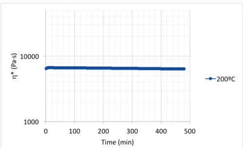
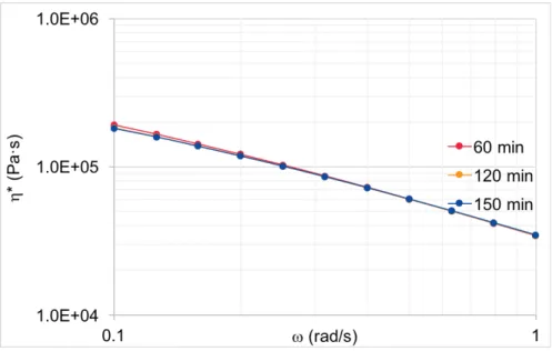
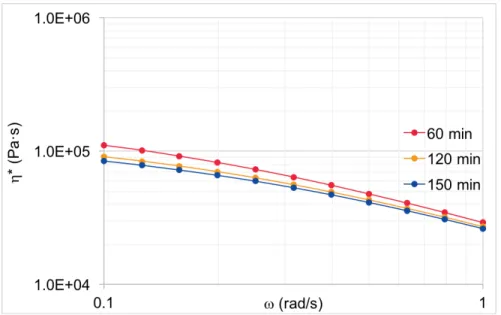
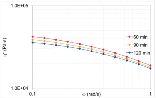
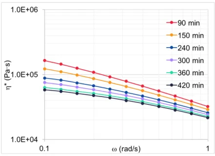
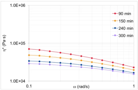
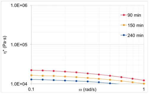
(13) List of Figures Figure I-1. Diagram of solution overview proposed for the present work. ........................ 6 Figure II-1. Parallel-plate geometry. ............................................................................... 14 Figure II-2. Free volume in function of temperature and demonstration of Vogel temperature. ............................................................................................................ 20 Figure III-1. Photograph of the high pressure rheometer. .............................................. 28 Figure III-2. Schematic of the high pressure cell rheometer. .......................................... 30 Figure III-3. Schematic of the experimental set up. ........................................................ 31 Figure III-4. Effect of the O-rings in the gap and frequency sweeps. (Screenshot taken from the Rheoplus/32 V3.62 software.) ................................................................... 37 Figure III-5. Flow chart for gauging gap. ........................................................................ 38 Figure III-6. Time sweep of complex viscosity (resin A) for 10% of strain, 5 rad/s, at 200ºC. ................................................................................................................................ 43 Figure III-7. Complex viscosity for different times of measurement at 170ºC and 6.89 MPa. ................................................................................................................................ 44 Figure III-8. Complex viscosity for different times of measurement at 185ºC and 6.89 MPa. ................................................................................................................................ 45 Figure III-9. Complex viscosity for different times of measurement at 200ºC and 6.89 MPa. ................................................................................................................................ 46 Figure III-10. Complex viscosity for different times of measurement at 170ºC and 13.78 MPa. ........................................................................................................................ 47 Figure III-11. Complex viscosity for different times of measurement at 185ºC and 13.78 MPa. ........................................................................................................................ 48 Figure III-12. Complex viscosity for different times of measurement at 200ºC and 13.78 MPa. ........................................................................................................................ 49 Figure IV-1. Torque measured for resin A at different temperatures. ............................. 52 Figure IV-2. Crossing of complex viscosity curves for resin A at different temperatures. ................................................................................................................................ 53 Figure IV-3. (A) Complex viscosity of resin A as obtained using the rheometer, and (B) adjusted complex viscosity using equation IV-3. ..................................................... 55 xi.

(14) Figure IV-4. Adjusted complex viscosity of resin A at different temperatures. ............... 56 Figure IV-5. Adjusted complex viscosity of resin A at different temperatures and atmospheric pressure, using equation IV-3. ............................................................ 57 Figure IV-6. Adjusted complex viscosity of resin A at different temperatures and 6.89 MPa of CO2, using equation IV-3. .................................................................................... 57 Figure IV-7. Adjusted complex viscosity of resin A at different temperatures and 13.78 MPa of CO2, using equation IV-3. ........................................................................... 58 Figure IV-8. Adjusted complex viscosity of resin B at different temperatures and atmospheric pressure, using equation IV-3. ............................................................ 58 Figure IV-9. Adjusted complex viscosity of resin B at different temperatures and 6.89 MPa of CO2, using equation IV-3. .................................................................................... 59 Figure IV-10. Adjusted complex viscosity of resin B at different temperatures and 6.89 MPa of CO2, using equation IV-3. ........................................................................... 59 Figure IV-11. Adjusted complex viscosity of resin C at different temperatures and atmospheric pressure, using equation IV-3. ............................................................ 60 Figure IV-12. Adjusted complex viscosity of resin C at different temperatures and 6.89 MPa of CO2, using equation IV-3. ........................................................................... 60 Figure IV-13. Adjusted complex viscosity of resin C at different temperatures and 13.78 MPa of CO2, using equation IV-3. ........................................................................... 61 Figure V-1. Negative ΔGM required for miscibility. (a) Intensive free energy of the mixture in function of mole fraction of component 2. (b) First derivative of the molar free energy in terms of chemical potential and mole fraction. ........................................ 72 Figure V-2. Binodal and spinodal curves for a polymer+SCF system (Adapted from [63]). ................................................................................................................................ 75 Figure V-3. Phase stability according to binodal and spinodal curves for a polymer+SCF system (Adapted from [63]). .................................................................................... 75 Figure V-4. Fitting of resin A + CO2 using Total’s model. ............................................... 78 Figure V-5. Fitting of resin B + CO2 using Total’s model. ............................................... 79 Figure V-6. Fitting of resin C + CO2 using Total’s model. ............................................... 80 Figure V-7. Diagram of the individual thermodynamic paths. ......................................... 82 Figure V-8. Diagram of possible thermodynamic paths based on experimental data. ... 84. xii.

(15) Figure V-9. Example of a thermodynamic path and shift factor equivalences. .............. 84 Figure V-10. Master curve of G* for resin A from data at 6.89 MPa. .............................. 88 Figure V-11. Master curve of tan(δ) for resin A from data at 6.89 MPa. ........................ 88 Figure V-12. Master curve of η* for resin A from data at 6.89 MPa. .............................. 89 Figure V-13. Master curve of η* for resin A from data at 13.78 MPa. ............................ 89 Figure V-14. Master curve of η* for resin A from data at 0.1 MPa. ................................ 93 Figure V-15. Example of adjustment of complex viscosity curve at 170ºC, 6.89 MPa, with no CO2 content (resin A). ........................................................................................ 97 Figure V-16. Example for obtaining concentration shift factor using viscosity curve at 170ºC, 6.89 MPa, with no CO2 content as reference (resin A). .............................. 98 Figure V-17. Demonstration of equivalence of individual paths versus direct superposition for resin A, from data at 6.89 MPa. ....................................................................... 102 Figure V-18. Matrix of elongational viscosities for PS resins at different temperatures and pressures, obtained from Cortés’ software. .......................................................... 109 Figure V-19. Steady state elongational viscosities for resin A at 200ºC and atmospheric pressure, obtained from Cortés’ software using data from different rheometers. . 112 Figure 1-1. Algorithm for the use of SLEOS. ................................................................ 130 Figure 5-1. Elongational viscosity versus time for different extensional rates and pressures at 170ºC, for resin A. ............................................................................ 167 Figure 5-2. Elongational viscosity versus time for different extensional rates and pressures at 185ºC, for resin A. ............................................................................ 168 Figure 5-3. Elongational viscosity versus time for different extensional rates and pressures at 200ºC, for resin A. ............................................................................ 169 Figure 5-4. Elongational viscosity versus time for different extensional rates and pressures at 170ºC, for resin B. ............................................................................ 170 Figure 5-5. Elongational viscosity versus time for different extensional rates and pressures at 185ºC, for resin B. ............................................................................ 171 Figure 5-6. Elongational viscosity versus time for different extensional rates and pressures at 200ºC, for resin B. ............................................................................ 172 Figure 5-7. Elongational viscosity versus time for different extensional rates and pressures at 170ºC, for resin C. ............................................................................ 173 xiii.

(16) Figure 5-8. Elongational viscosity versus time for different extensional rates and pressures at 185ºC, for resin C. ............................................................................ 174 Figure 5-9. Elongational viscosity versus time for different extensional rates and pressures at 200ºC, for resin C. ............................................................................ 175. xiv.

(17) List of Tables Table I-1. Comparison table identifying contributions on the research field. .................... 7 Table III-1. MWD data for PS resins. .............................................................................. 27 Table III-2. DSC data for PS resins. ............................................................................... 27 Table III-3. Anton Paar SmartPave MCR101 technical specifications. .......................... 29 Table III-4. Calculation of the empirical volumetric thermal expansion coefficient. ........ 35 Table III-5. Samples’ dimensions used for the study. ..................................................... 35 Table III-6. Reported values for linear (a) and volumetric thermal expansion coefficient (bT) for PS at different temperatures. ...................................................................... 36 Table III-7. Solubilities for CO2 in PS at various temperatures and pressures. .............. 40 Table III-8. Binary interaction parameter for PS+CO2 at different temperatures reported by Sato et al [43]. .................................................................................................... 40 Table III-9. Predicted binary interaction parameter for PS+ CO2 at different temperatures, using equation III-3. ................................................................................................. 41 Table III-10. Swelling ratios for PS+CO2 at various temperatures and pressures using equation III-7. .......................................................................................................... 42 Table III-11. Summary of equilibrium time and at 170ºC and 6.89 MPa, and relative percentage of difference between sweeps. ............................................................. 44 Table III-12. Summary of equilibrium time and at 185ºC and 6.89 MPa, and relative percentage of difference between sweeps. ............................................................. 45 Table III-13. Summary of equilibrium time and at 200ºC and 6.89 MPa, and relative percentage of difference between sweeps. ............................................................. 46 Table III-14. Summary of equilibrium time and at 170ºC and 13.78 MPa, and relative percentage of difference between sweeps. ............................................................. 47 Table III-15. Summary of equilibrium time and at 185ºC and 13.78 MPa, and relative percentage of difference between sweeps. ............................................................. 48 Table III-16. Summary of equilibrium time and at 200ºC and 13.78 MPa, and relative percentage of difference between sweeps. ............................................................. 49 Table III-17. Summary of equilibrium times at 6.89 MPa ............................................... 50 Table III-18. Summary of equilibrium times at 13.78 MPa ............................................. 50. xv.

(18) Table IV-1. Experimental parameters used for high pressure rheological tests. ............ 51 Table V-1. SLEOS sensitivity to binary interaction parameter. ...................................... 64 Table V-2. Comparison of solubility correlations using different EOS. ........................... 65 Table V-3. Percentages of differences between estimations from EOS. ....................... 65 Table V-4. Characteristic parameters for PS and CO2 used in SLEOS. ........................ 66 Table V-5. Critical properties of CO2. ............................................................................. 67 Table V-6. Densities of CO2 at different temperatures and pressures. .......................... 67 Table V-7. Constants to calculate density of PS at atmospheric pressure. .................... 68 Table V-8. Constants to calculate density of PS in function of temperature and pressure. ................................................................................................................................ 69 Table V-9. Comparison of densities of PS at different temperatures and pressures. .... 69 Table V-10. SLEOS results regarding free volume and density. .................................... 70 Table V-11. SLEOS Thermodynamics of mixing for PS+CO2 at different temperatures and pressures. ............................................................................................................... 74 Table V-12. Significant results from Total’s model for PS+CO2 systems. ...................... 77 Table V-13. Compounded shift factors calculated for resin A. ....................................... 86 Table V-14. Compounded shift factors calculated for resin B. ....................................... 86 Table V-15. Compounded shift factors calculated for resin C. ....................................... 87 Table V-16. Proof of equivalence of compounded shift factors for resin A. ................... 90 Table V-17. Proof of equivalence of compounded shift factors for resin B. ................... 90 Table V-18. Proof of equivalence of compounded shift factors for resin C. ................... 90 Table V-19. Fractional free volumes with respect to occupied volume (fD) for PS. ....... 91 Table V-20. Temperature shift factors for PS resins. ..................................................... 92 Table V-21. Constants for Kovacs’ equation. ................................................................. 93 Table V-22. Evaluation of predicted aT versus empirical. ............................................... 94 Table V-23. Predicted values for pressure shift factors. ................................................. 95 Table V-24. Predicted values for concentration shift factors. ......................................... 96 Table V-25. Evaluation of quasi-empirical aC versus derived for resin A. ...................... 98 Table V-26. Evaluation of quasi-empirical aC versus derived for resin B. ...................... 99 Table V-27. Evaluation of quasi-empirical aC versus derived for resin C. ...................... 99 Table V-28. Summary of equations used to estimate shift factors. .............................. 100. xvi.

(19) Table V-29. Evaluation of compounded shift factors for resin A. ................................. 100 Table V-30. Evaluation of compounded shift factors for resin B. ................................. 100 Table V-31. Evaluation of compounded shift factors for resin C. ................................. 101 Table V-32. Plateau moduli and Me for resin A. ........................................................... 106 Table V-33. Plateau moduli and Me for resin B. ........................................................... 106 Table V-34. Plateau moduli and Me for resin C. ........................................................... 106 Table V-35. Discrete relaxation spectrum obtained from Mier’s software for resins at 0.1 MPa. ...................................................................................................................... 107 Table V-36. Discrete relaxation spectrum obtained from Mier’s software for resins at 6.89 MPa. ...................................................................................................................... 107 Table V-37. Discrete relaxation spectrum obtained from Mier’s software for resins at 13.78 MPa. ...................................................................................................................... 108 Table V-38. Times to reach elongational viscosity steady state. .................................. 110 Table 2-1. Frequency sweep for resin A at 170ºC, 14.7 psi. ........................................ 131 Table 2-2. Frequency sweep for resin A at 185ºC, 14.7 psi. ........................................ 132 Table 2-3. Frequency sweep for resin A at 200ºC, 14.7 psi. ........................................ 133 Table 2-4. Frequency sweep for resin A at 170ºC, 1000 psi. ....................................... 134 Table 2-5. Frequency sweep for resin A at 185ºC, 1000 psi. ....................................... 135 Table 2-6. Frequency sweep for resin A at 200ºC, 1000 psi. ....................................... 136 Table 2-7. Frequency sweep for resin A at 170ºC, 2000 psi. ....................................... 137 Table 2-8. Frequency sweep for resin A at 185ºC, 2000 psi. ....................................... 138 Table 2-9. Frequency sweep for resin A at 200ºC, 2000 psi. ....................................... 139 Table 2-10. Frequency sweep for resin B at 170ºC, 14.7 psi. ...................................... 140 Table 2-11. Frequency sweep for resin B at 185ºC, 14.7 psi. ...................................... 141 Table 2-12. Frequency sweep for resin B at 200ºC, 14.7 psi. ...................................... 142 Table 2-13. Frequency sweep for resin B at 170ºC, 1000 psi. ..................................... 143 Table 2-14. Frequency sweep for resin B at 185ºC, 1000 psi. ..................................... 144 Table 2-15. Frequency sweep for resin B at 200ºC, 1000 psi. ..................................... 145 Table 2-16. Frequency sweep for resin B at 170ºC, 2000 psi. ..................................... 146 Table 2-17. Frequency sweep for resin B at 185ºC, 2000 psi. ..................................... 147 Table 2-18. Frequency sweep for resin B at 200ºC, 2000 psi. ..................................... 148. xvii.

(20) Table 2-19. Frequency sweep for resin CX 5299 at 170ºC, 14.7 psi. .......................... 149 Table 2-20. Frequency sweep for resin CX 5299 at 185ºC, 14.7 psi. .......................... 150 Table 2-21. Frequency sweep for resin CX 5299 at 200ºC, 14.7 psi. .......................... 151 Table 2-22. Frequency sweep for resin CX 5299 at 170ºC, 1000 psi. ......................... 152 Table 2-23. Frequency sweep for resin CX 5299 at 185ºC, 1000 psi. ......................... 153 Table 2-24. Frequency sweep for resin CX 5299 at 200ºC, 1000 psi. ......................... 154 Table 2-25. Frequency sweep for resin CX 5299 at 170ºC, 2000 psi. ......................... 155 Table 2-26. Frequency sweep for resin CX 5299 at 185ºC, 2000 psi. ......................... 156 Table 2-27. Frequency sweep for resin CX 5299 at 200ºC, 2000 psi. ......................... 157 Table 4-1. Constants for pressure shift factor (I) for PS resins. ................................... 165 Table 4-2. Constants for pressure shift factor (II) for PS resins. .................................. 165. xviii.

(21) Contents Dedication.................................................................................................................... v Acknowledgements .................................................................................................. vii Abstract ...................................................................................................................... ix List of Figures ............................................................................................................ xi List of Tables ............................................................................................................. xv Nomenclature ......................................................................................................... xxiii. Chapter I ...................................................................................................... 1 I.. Introduction .......................................................................................................... 1 1.. Motivation ........................................................................................................... 1. 2.. Problem statement and context ......................................................................... 3. 3.. Research proposal and objectives ..................................................................... 3. 4.. Justification ........................................................................................................ 4. 5.. Solution Overview .............................................................................................. 5. 6.. Main Contributions ............................................................................................. 7. 7.. Methodology ...................................................................................................... 8 A.. Material characterization ................................................................................ 8. B.. Sample preparation ........................................................................................ 9. C. Oscillatory rheology ........................................................................................ 9 D. Data analysis .................................................................................................. 9 8.. Dissertation Organization ................................................................................... 9. Chapter II ................................................................................................... 11 II.. Theoretical background .................................................................................... 11 1.. Polymeric Foams ............................................................................................. 11. 2.. Manufacturing .................................................................................................. 12. 3.. High-pressure rheology .................................................................................... 13 A.. Rheological measurements .......................................................................... 14. 4.. Time-Temperature Superposition and related models ..................................... 17. 5.. Equation of States ............................................................................................ 23 xix.

(22) A.. Cubic EOS .................................................................................................... 23. B.. Lattice fluid theory ........................................................................................ 24. C. Off-lattice fluid theory .................................................................................... 26. Chapter III .................................................................................................. 27 III.. Experimental materials and methods .......................................................... 27. 1.. Materials........................................................................................................... 27. 2.. Equipment ........................................................................................................ 28. 3.. Experimental set up ......................................................................................... 31. 4.. Oscillatory rheology ......................................................................................... 32. 5.. Sample preparation .......................................................................................... 33. 6.. Experimental method ....................................................................................... 33 A.. Sample dimensions ...................................................................................... 34. B.. Gap ............................................................................................................... 36. C. Sample deformations .................................................................................... 39 D. Degradation .................................................................................................. 42 E.. Time of measurement .................................................................................. 43. F.. Additional considerations ............................................................................. 50. Chapter IV.................................................................................................. 51 IV.. Results and treatment of data....................................................................... 51. 1.. Frequency sweeps ........................................................................................... 51. 2.. Adjustment of data ........................................................................................... 53 A.. Correction for volume ................................................................................... 54. B.. Correction for thermal expansion ................................................................. 54. C. Correction for swelling .................................................................................. 54 3.. Results ............................................................................................................. 56 A.. Resin A ......................................................................................................... 57. B.. Resin B ......................................................................................................... 58. C. Resin C ......................................................................................................... 60. xx.

(23) Chapter V................................................................................................... 63 V.. Analysis and discussion ................................................................................... 63 1.. SLEOS evaluation ............................................................................................ 63 A.. Binary interaction parameter ........................................................................ 64. B.. Solubility correlation ..................................................................................... 65. C.. Material’s properties ................................................................................. 66. D.. Mixture properties ..................................................................................... 70. E.. Phase stability .............................................................................................. 71. 2.. Total’s high pressure rheology model .............................................................. 76. 3.. Time-temperature-pressure-concentration superposition ................................ 81. 4.. A.. Compounded shift factors ............................................................................ 85. B.. Effect of temperature .................................................................................... 92. C.. Effect of pressure ...................................................................................... 94. D.. Effect of concentration .............................................................................. 95. E.. Evaluation of shift factors ........................................................................... 100 Relaxation spectra and elongational viscosity ............................................... 103. Chapter VI................................................................................................ 113 VI.. Conclusions.................................................................................................. 113. 1.. Findings and conclusions ............................................................................... 113. 2.. Recommendations and future work ............................................................... 116. Bibliography............................................................................................ 119 Appendix A.............................................................................................. 127 1). Complementary SLEOS – equations. ............................................................ 127. Appendix B.............................................................................................. 131 2). Experimental data. ........................................................................................... 131. Appendix C.............................................................................................. 159 3). SLEOS – Algorithm for Polymath................................................................... 159. Appendix D.............................................................................................. 165 4). Constants for pressure shift factor modeling............................................... 165 xxi.

(24) Appendix E .............................................................................................. 167 5). Elongational viscosity versus time. ............................................................... 167. Curriculum Vitae ..................................................................................... 177. xxii.

(25) Nomenclature Symbols: BHT 2,6-Di-tert-butyl-4-methylphenol. 𝐴/ , 𝑎/ Constants. CBA Chemical blowing agent. 𝐴2. CFCs Chlorofluorocarbons. model). CNC Computer Numerical Control CO2. 𝐴32. Carbon dioxide. 𝑎4. EOS Equation of state Hydrochlorofluorocarbons Molecular weight distribution. Perturbed-chain-SAFT. PR. Peng-Robinson. PVT. Pressure-volume-temperature. 𝑎3,5. Horizontal pressure-concentration. concentration shift factor. PBA Physical blowing agent Polystyrene. Horizontal pressure shift factor. 𝑎 2,3,5 Horizontal temperature-pressure-. model. PS. 𝑎3. shift factor. NRHB Non-random Hydrogen-bonding. PC-SAFT. Horizontal concentration shift. factor. GPC Gel Permeation Chromatography MWD. Pressure-temperature parameter. (Total’s model). DSC Differential scanning calorimetry. HCFCs. Temperature parameter (Total’s. 𝑎2. Horizontal temperature shift factor. 𝑎 2,5. Horizontal temperature-. concentration shift factor 𝐵. Constant. 𝑏. Solubility parameter. bonding. 𝑏/. Constant. SAFT Statistical association fluid theory. 𝑏38. Peng-Robinson parameter. SCF Supercritical fluid. 𝑏2,3,5 Vertical temperature-pressure-. SC-CO2. Supercritical carbon dioxide. concentration shift factor. SLEOS. Sanchez-Lacombe equation. 𝑏2. Vertical temperature shift factor. of state. 𝐶. Constant. TTSP Time-temperature superposition. 𝑐. Parameter (Total’s model). WLF Williams-Landel-Ferry. 𝑐; , 𝑐< Constants. QHCB. Quasi-chemical Hydrogen-. xxiii. 𝐸>. Activation energy. 𝑓. Fractional free volume.

(26) 𝑓@. 𝑛. Carreau-Yasuda constant. reference condition. 𝑃4. Critical pressure. 𝑓A. 𝑃∗. Characteristic pressure. respect to the occupied volume. ∗ 𝑃VQW. Characteristic pressure of the. (Doolittle’s). mixture. 𝑓B. 𝑃. Fractional free volume at Fractional free volume with. Fractional free volume with. respect to the total volume. Reduced pressure (characteristic pressure). 𝑓C. Fractional occupied volume. 𝑅. Radius. 𝐺. Intensive free energy. 𝑟. Number of lattice occupied by a. 𝐺’. Storage modulus. 𝐺’’. Loss modulus. 𝐺∗. Complex modulus. 𝐻. Gap. molecule 𝑟Q@. Number of lattice occupied by a molecule in the pure state. 𝑅Z. Gas constant. 𝐻(𝜆) Relaxation spectrum. 𝑡. Time. 𝑘. Peng-Robinson parameter. 𝑇. Temperature. 𝑘3. Henry's law constant. 𝑇∗. Characteristic temperature. 𝑘J. Boltzman constant. 𝑇. Reduced temperature. 𝑘;<. Binary interaction parameter. 𝑀. Torque. 𝑇@. Reference temperature. 𝑀L. Average molecular weight. 𝑇4. Critical temperature. between entaglements. 𝑇]. Glass transition temperature. 𝑀/. 𝑇^. Reduced temperature. 𝑇_. Vogel temperature. 𝑉. Volume. 𝑉∗. Characteristic volume of the. (characteristic temperature). Number-averaged molecular. weight 𝑀M. Weight-averaged molecular. weight 𝑀𝑊. Molecular weight. mixture. 𝑀O. Z-averaged molecular weight. 𝑉4a. Volume of cylinder. 𝑚Q. Mass fraction. 𝑉b. Final volume. 𝑚3R. Mass of PS. 𝑉VQW. Volume of the mixture. 𝑁. Total number of moles. 𝑉@. Initial volume. 𝑁@. Empty sites xxiv.

(27) 𝑥. Mole fraction. 𝛾@. Strain. 𝑧. Coordination number. 𝜂. Shear viscosity. 𝜂∗. Complex viscosity. Greek symbols:. 𝜂@. Zero shear viscosity. 𝛼. 𝜂]. Viscosity at glass transition. Linear thermal expansion. coefficient. temperature. 𝛼A. Damping function (m-PPT). 𝜆. Relaxation time. 𝛼B. Thermal expansion coefficient of. 𝜇. Chemical potential. free volume. 𝛺. Angular velocity. 𝛽. Isothermal compresibility. ω. Frequency. 𝛽B. Compressibility coefficient of free. 𝜔>. Acentric factor. volume. 𝜌. density. 𝛽2. 𝜌∗. Characteristic density. coefficient. 𝜌. Reduced density. 𝛥𝑇. Temperature difference. 𝜌t. Polymer density. 𝛥𝑃. Pressure difference. 𝜌3R. Polystyrene density. 𝛥𝐺h. Gibbs free energy of mixing. 𝜌u. Solvent density. 𝛥𝐻h. Enthalpy of mixing. 𝜏. Stress tensor. 𝛥𝑆h. Entropy of mixing. 𝜏u. Shear stress. 𝛿. Phase angle. 𝜏8. Carreau-Yasuda constant. 𝜖∗. Characteristic energy of. 𝜏OO , 𝜏WW. Volumetric thermal expansion. Stress components. interaction per mer. 𝜐. Reduced volume. 𝜙. Close-packed volume fraction. 𝜐∗. Close-packed mer volume. 𝜙Q@. Close-packed volume fraction of. (characteristic volume) ∗ 𝜐ut. the molecule in the pure state 𝛾. Shear rate. xxv. Specific volume.

(28) xxvi.

(29) Chapter I I. Introduction 1.. Motivation. Today the tailoring of materials should take as little time as the market needs change, however that requires a lot of work, time, economic and material resources. Since every company in the polymer industry makes profit from mass production, it is imperative to develop methods that can shorten the testing and prototyping phase whenever a new product is being developed. Therefore, having a method to achieve such customization constitutes the most valuable tool on materials engineering. The real challenge relies on understanding the physical-chemical phenomena behind the manufacturing process in such way that the generated knowledge can be used in convenience of the material designer. From this premise emerges the driving force to generate models that work as mechanisms for the development of new products with fitted properties. The extrusion of polymeric foams using supercritical fluids (SCFs) as blowing agents involves the interaction of different variables at once such as residence time, temperature and pressure. These will determine the degree of saturation and mixing of the polymer and the blowing agent, same that impact on the resin’s viscoelastic properties and consequently on the foaming behavior of the mixture. Nevertheless, differences in molecular weight distribution, chemical composition and/or additives content may produce varieties of polymeric foams. Running batches for each combination is challenging and expensive.. 1.

(30) Although there are some models for high pressure rheology that can predict viscosities for extrusion operating conditions, they fail to isolate the effect of temperature, pressure and diluent concentration in the mixture. Thus, it is hard to quantitatively identify the effect of the operating conditions on the viscoelastic properties of the polymer prior to the foam extrusion. Having a model that can accurately predict the rheological behavior of polymer melts on high pressures and temperatures would help to reduce the time and resources invested on testing polymer melts in the foam line, or even identify desirable or undesirable rheological behaviors before escalating it into a pilot plant. Nonetheless, in order to generate a model for such purpose, or even make conclusions towards foaming applications, it is essential to acquire reliable experimental data. Such task becomes challenging when dealing with high pressures and supercritical fluids, mainly due to a lack of appropriate equipment for high pressure rheology. Efforts have been made to design high pressure rheometers to measure viscoelastic properties of polymer melts, such as the slit die rheometer by Han [1], but pressure gradients are hard to control. An alternative has been developed using a parallel plate rheometer inside a pressure cell, but troubles regarding gap control, and therefore repeatability, have been reported [2]. Therefore, in the view of the challenge on data acquisition it is necessary to develop a methodology that can provide accurate rheological measurements. On the other hand, this study also finds its motivation on the pursuit of processes and materials with a lower environmental impact, particularly on the polymeric foam industry. This can be achieved by helping to understand the effects and foaming phenomena associated with the use of carbon dioxide (CO2) to encourage its massive use in order to displace the gases currently used on the industry that causes depletion of the ozone layer.. 2.

(31) 2.. Problem statement and context. Understanding the mixing of supercritical fluids in a polymer matrix requires accurate measurements of viscoelastic properties under high pressures and temperatures, but available equipment consisting in a parallel plate rheometer in a pressure cell incurs errors related to design and sensitivity [2], [3]. Therefore, a proper methodology for experimentation and adjustment of data are needed in order to acquire useful rheological data. On the other hand, to comprehend the foaming behavior of a polymer melt it is necessary the prediction of elongational viscosity, which is an important factor for bubble growth, same that regulates the foam morphology or structure [4], [5]. However, little research has been done in this matter for its complexity for testing. Therefore, the prediction of the extensional viscosity through obtainable rheological data and validated models, is desired. Finally, given the combination of factors involved in foam extrusion, the identification and isolation of temperature, pressure and concentration effects on viscoelastic properties of polymer melts are needed to develop a predictive model using standard rheology and polymer characterization tests. 3.. Research proposal and objectives. In the interest of having a quantitatively and better understanding about polymers foaming, the solubility of SC-CO2 in polystyrene (PS) and the effect of the dissolved gas on melt rheology will be studied. The main objective of this research is to develop a testing methodology that can provide accuracy and repeatability for high pressure oscillatory rheology tests. In addition, it is intended to develop a model that settles the basis for the prediction of viscoelastic properties of polymer melts for foaming applications.. 3.

(32) 4.. Justification. Polymeric foams are adaptable materials used for various purposes depending mainly on their cell morphology and density. These materials are produced from adding a blowing agent into a molten polymer. Polymeric foams can be made of open or closed-cell structures which will determine physical properties such as stiffness, density and insulation capacity. Since their variations cover from soft to high-impact foams, polymeric foams can be found in airplanes and automotive parts, as acoustic or thermal insulators for construction or appliances, and as varieties of cushioning for furniture or packaging to avoid product damage. One of the most important methods for producing polymeric foams is the extrusion process using SCFs as blowing agent. In this method, a polymer is mixed with a SCF as the polymer melts under high pressures inside a barrel. Once a homogenous mix is achieved, the polymer blend is pushed forward by a screw, exits through a die and expands as a result of the depressurization. In order to produce polymeric foams with specific properties, the foaming process phenomena has to be understood as well as the viscoelastic behavior of the high pressure polymer-SCF system. The production process of polymeric foams has changed mainly due to environmental concerns about the use of chlorofluorocarbons (CFCs) as blowing agents. These issues have taken importance on the last decades because of global warming and the deterioration of the ozone layer. In order to encourage the atmospheric protection, traditional blowing agents such as CFCs have been banned from the plastic industry, and a similar future awaits their replacements; the hydrochlorofluorocarbons (HCFCs). Today, SC-CO2 is known to be a good solvent for obtaining foams with attractive properties. It represents a suitable alternative as blowing agent for it is easily found in the atmosphere and thus inexpensive, it is also chemically stable and nonflammable.. 4.

(33) Other advantages offered by SC-CO2 are related to its effect on the polymer properties. SC-CO2 acts as plasticizer on polymer melts by reducing their viscosity due to an increase on the free volume and so, it affects also their density and swollen volume. During the extrusion process it is crucial to maintain CO2 concentrations above its solubility limit to avoid phase changes inside the barrel, therefore it is important to know the equilibrium data for each system in order to control de process; however, there is limited data about CO2 solubility on polymer systems at supercritical conditions. Recent investigations suggest that the number and size of cells, as well as their distribution are defined by process conditions: saturation pressure, saturation temperature and depressurization rate, whereas polymer’s viscoelasticity and interfacial tension regulate the cell size by avoiding elongation of the cells during growth [5], [6], [7]. Given the importance of the viscoelastic properties of the polymer melt under high pressure and temperatures, it is relevant to be able to predict those properties in order to correlate them with a foaming behavior. 5.. Solution Overview. It is intended to develop a testing methodology to provide accuracy and repeatability on rheology testing using a parallel-plate rheometer in a pressure cell, based on the phenomena explained by the Sanchez-Lacombe Equation of State (SLEOS) [8]. Moreover, it is believed that a model based on the time-temperature superposition principle can be formulated to predict viscoelastic properties of polystyrene-CO2 systems to have a better understanding of the foaming behavior of polymer melts. Outputs from both approaches would be used to forecast the elongational viscosity in order to determine which polymers would exhibit better foamability and settle the basis for a deeper foam extrusion study.. 5.

(34) Figure I-1. Diagram of solution overview proposed for the present work.. 6.

(35) 6.. Main Contributions. The ultimate contribution of this study is the proposal of a predictive model for viscoelastic properties of polystyrene-CO2 systems that also settles the basis for future correlations between high pressure rheology and foam extrusion using SCFs. Thus, the findings of these experiments will be translated into a method to quantify the effects of the blowing agent on the rheological properties of the polymers under high pressures and by consequence; the discernment of the proper window of operating conditions for polystyrene foaming. Table I-1 identifies the contributions of this research based on the findings and objectives fulfilled in this study. Table I-1. Comparison table identifying contributions on the research field.. 1999 Lee et al. [9] 2000 2006 2009 2012 2015 2016. PS. Royer et al. PS [10] Park and HDPE Dealy [11] Wingert et PS al. [3] Handge and PS Altsädt [2] Gutierrez et PS al. [12] Present PS work. ✓ ✓. ✓. ✓. ✓. ✓. ✓. ✓. ✓. ✓ ✓. ✓. ✓. 7. 3.5 – 25.1 MPa ✓ 220ºC 8.6 – 14.8 MPa ✓ ✓ ✓ 200 – 250ºC 0.1 – 70 MPa ✓ ✓ ✓ 180ºC 0.1 – 13.9 MPa ✓ ✓ ✓ ✓ 140 – 180ºC 0.1 - 5 MPa ✓ ✓ ✓ 130 - 170ºC 0.1 – 20 MPa ✓ ✓ ✓ 30 – 100ºC 0.1 - 13.78 MPa ✓ ✓ ✓ ✓ 170 - 200ºC. elongational viscosity. CO2 concentration. Temperature. Pressure. Operating conditions. Complex viscosity. Research. Variables. High-pressure rheology Thermodynamics of the mixture Prediction of viscoelastic properties. Year. Polymer. Topics. ✓.

(36) 7.. Methodology. The main rheology tests will consist of high pressure oscillatory tests performed with a parallel-plate rheometer adapted inside a pressure cell that allows to pressurize polymer samples with SC-CO2. Data recollected from oscillatory tests will be analyzed in order to determine the appropriate treatment so it can be used as input for the development of a predictive model. Furthermore, experimental data will be compared with reported values on literature to validate models and parameters used for data analysis and estimations. Conclusions about the impact of CO2 in the polymer’s viscoelastic properties will be drawn based on the identification of temperature, pressure and concentration effect for three different polystyrene samples. Finally, elongation viscosity will be calculated using Mier’s [13] and Cortés’ [14] models as it is relevant for future correlations between high pressure rheology and foaming behavior, specially via foam extrusion. In general terms, the methodology used on this study consisted of: A.. Material characterization. Standard characterization methods were performed for each sample such as gel permeation chromatography (GPC) for molecular weight distribution data, and differential scanning calorimetry (DSC) for glass transition temperature valuation.. 8.

(37) B.. Sample preparation. All resins were molded from pellets into plaques with the same protocol using a molding press with controlled cooling system. Sample dimensions were determined for appropriate testing in a parallel-plate rheometer. C.. Oscillatory rheology. All oscillatory tests were performed using a parallel-plate rheometer at same frequencies and percentage of strain. Test were made at three temperatures and two different pressures, additionally to atmospheric pressure. For specific procedures, details will be explained in Chapter III. D.. Data analysis. Treatment of data was required to correct experimental results to make them useful for modeling. Predictive models were proposed by isolating effects of temperature, pressure and concentration on viscoelastic properties. Additional calculations were made for estimation of elongational viscosity to draw preliminary conclusions about foaming behavior of PS resins. 8.. Dissertation Organization. This thesis is divided in six chapters, including the present one of introduction. Chapter II starts with a literature review, covering some topics about polymeric foams and high pressure rheology. Chapter III contains descriptions of the experimental protocol and experimental set ups. It explains the methodology used for testing and the considerations required to assure repeatability and constancy.. 9.

(38) Chapter IV presents the results from oscillatory rheology and explains the developed methodology for the data treatment. Corrected frequency sweeps for each resins are plotted and some preliminary analysis is made. Chapter V comprises the discussion of the results and the evaluation of the models used for the data treatment. Two approaches are used to identify, measure and compare the effect of temperature, pressure and CO2 concentration on the viscoelastic properties of the PS resins. The first one involves a high pressure rheology model developed by Total Petrochemicals & Refining USA, Inc., and the second one consists on a timetemperature-pressure-concentration superposition. Additionally, a preliminary study of elongational viscosity will be presented to have an insight about how the resins behave under extensional rates, which are directly related to bubble’s growth. Finally, Chapter VI presents general conclusions about the research, a brief summary of the findings, additional comments about high pressure rheology and recommendations for future work.. 10.

(39) Chapter II This chapter contains a literature review, including manufacturing aspects of polymeric foams that justify the use of high pressure rheology and some models that help to understand the viscoelastic behavior of polymer-SCF systems. In addition, some equations that will be used in the study are presented in the context of high pressure rheology. Note that some nomenclature varies from the original versions in order to be consistent with notations and allow compatibility of models along the document.. II. Theoretical background 1.. Polymeric Foams. During the past century, the plastic industry developed fast due to plastics’ exceptional properties and their capacity to replace fragile materials, moreover the improvement of new processes to synthesize thermoplastic and thermosetting plastics encouraged the growth of the polymeric foam industry. The technology evolution and the rising interest on polymeric foams by the early thirties with the invention of the polystyrene foam, helped to bring the industry to its peak four decades later. During that period the foam extrusion, injection and foam expansion were the main process used on the industry and therefore they reached maturity by the late eighties [15]. Dow Chemical, Trexel and DuPont were the first companies on improving the foaming methods up to the present, to even achieving the production of microcellular foams. However, it could be said that the use of SCFs, for instance SC-CO2, as blowing agent in the industry has been recent since they were introduced as the result from the displacement of CFCs by the 1990s.. 11.

(40) Even when this variation on supplies does not represent a revolutionary change in the foaming process, the use of inert gases as blowing agents opens a window of opportunity on the market to develop cheaper processes with lower manufacturing costs, using inexpensive and environmental friendly materials. 2.. Manufacturing. Polymeric foams are produced from mixing a polymer resin or blend with a blowing agent in order to obtain gaseous voids dispersed in the matrix. Their properties will depend on some structural parameters such as cell density, open-cell content and cell distribution, which will be determined by the manufacturing process and operating conditions. There are two main methods to manufacture polymeric foams: reactive foaming and soluble foaming. The first one involves mixing a polymer with a chemical blowing agent (CBA) that decomposes into a gas by chemical reactions or thermal decomposition. The former consists on dissolving a physical blowing agent (PBA) in a polymer melt to achieve a homogeneous solution, then a depressurization of the system is produced to boost foaming as the PBA is released from the matrix [15]. The advantage of using soluble foaming is that it can be used on continuous foaming. The most used method for continuous foam processing is the foam extrusion. Extrusion is a continuous process in which a moldable material is shaped by driving it out with pressure through an orifice with the desirable contour in order to obtain objects with fixed cross-sectional profile. Polymeric foam extrusion can be divided in three major steps: (1) Mixing of polymer melt and PBA into a homogenous solution; (2) cell nucleation caused by a thermodynamic instability either by temperature and/or pressure; (3) foaming of polymer matrix by cell growth and coalescence [16]. This study will be focused on the first step that involves the plasticization of the melt by injecting SC-CO2 as blowing agent.. 12.

(41) SCFs have been adopted as attractive blowing agents on polymer processing during the last decade because they offer advantages such as gas-like diffusivity, liquid-like density and low viscosity [17]. Supercritical carbon dioxide stands out as a good alternative for substituting the CFCs and HCFCs because it is inflammable, non-toxic, inexpensive, chemically stable (inert gas) and has easily accessible supercritical conditions (Tc=304 K, Pc=7.38 MPa) [18]. Moreover, SC-CO2 happens to be a plasticizer, thus dissolved SC-CO2 on polymer melts decreases viscosity [3], [9], [10], and alters other physical properties including density, interfacial tension and glass transition temperature [10], [19]–[21]. Another advantage of using SCF on foam extrusion is the avoiding of increasing the processing temperature because of the decrease on melt viscosity and 𝑇] , so the energy consumption is lower and thermal degradation of the polymer is prevented. In foam extrusion the use of SCCO2 has an evident impact on the final product since it affects polymer properties directly related to the mechanisms of cell nucleation and cell growth [16]. 3.. High-pressure rheology. Established models for predicting rheological properties of a polymer melt, such as SLEOS [8], Doolittle’s [22], Carreau-Yasuda’s [23], WLF equation [24], among others, have been used widely by many investigators to generate other models or theories about the effects of temperature, pressure and/or solvent concentration, generally through empirical parameters by fitting the experimental data. This is the case, for example, of proposals from Royer et al. [10], Wingert et al. [3], Lee et al. [9] and Nobelen et al [25], whose studies are based on these prevalent equations to accurately predict melt viscosity in function of free volume and glass transition temperature. To address explanations about different approaches on high-pressure rheology for polymer melts, first it will be exposed some basic principles of rheology and the most adapted models on recent decades for high-pressure rheology.. 13.

(42) A.. Rheological measurements. The simplest way to measure rheological properties of fluids in function of rate of deformation is by imposing a shearing flow or shearing stress [26]. There are different types of geometries for imposing shearing flow, either by drag or pressure flow. For drag flows there are: sliding plates, concentric cylinders, cone and plate and parallel disks geometries. For pressure flows it can be used the capillary, slit or axial annulus geometry. For high pressure rheology one can adapt different geometries for drag and pressure flows. The most used rheometer consist in a slit die rheometer first adapted by Han [1] and later used by Han and Ma [27], Royer et al. [10], Lee et al. [9] and Lee et al. [21], among others. Others have used a Couette rheometer (concentric cylinders) [3] and even a parallel-plate [2], [3]. However, these last ones are hard to adapt to high pressure environments and therefore to use them for accurate measurements. The parallel-plate geometry will be the one used for this study, therefore it is relevant to mention the basis of this instrument. (i). Shearing flow. A parallel-plate rheometer (Figure II-1) consists of two parallel concentric disks separated by a fixed gap. During testing, one of the plates rotates while torque and normal force are measured by either one of them [28].. Figure II-1. Parallel-plate geometry. 14.

(43) For a parallel-plate rheometer, the shear rate (𝛾) will depend on the angular velocity (𝛺), sample radius (R) and gap (H), while the shear stress (𝜏u ) will depend on the same variables and the torque (M), as following:. 𝛾=. 𝛺𝑅 𝐻. (II-1). 𝜏u =. 2𝑀 𝜋𝑅{. (II-2). Then, the steady-state shear viscosity is obtained by:. 𝜂(𝛾) =. 𝜏u 𝛾. (II-3). In oscillatory rheology the shear rate is a sinusoidal function of time and so is the strain, therefore the shear stress produced by the deformation varies in time as well. Then the viscosity calculated via oscillatory shearing is called “complex viscosity”:. 𝜂∗ (𝜔) =. 𝜏u 𝑡 𝛾 𝑡. (II-4). However, according to the so-called “Cox-Merz rule” [29], for many polymer melts the shear viscosity as a function of shear rate equals the complex viscosity as a function of frequency [26] when frequency is in rad/s: 𝜂∗ 𝜔 ≡ 𝜂(𝛾). 15. (II-5).

(44) (ii). Storage and Loss Moduli. As previously said, when using oscillatory rheology, the stress varies sinusoidally with time and it is proportional to the amplitude of the strain according to: 𝜏u 𝑡 = 𝛾@ 𝐺 } 𝜔 sin 𝜔𝑡 + 𝐺 }} 𝜔 cos 𝜔𝑡. (II-6). Where 𝐺′ is the storage modulus that represents the storage of elastic energy, and 𝐺′′ is the loss modulus that represents the viscous dissipation of the same energy [26]. These can be expressed in terms of relaxation times (𝜆) or relaxation spectrum 𝐻(𝜆), as: _. 𝜔𝜆 < 𝐺 𝜔 = 𝐻 𝜆 1 + 𝜔𝜆 ‡_ }. 𝐺 }} 𝜔 =. _. 𝐻 𝜆 ‡_. 𝜔𝜆 1 + 𝜔𝜆. 𝑑 ln 𝜆 <. 𝑑 ln 𝜆 <. (II-7). (II-8). Relevant information can be obtained by these moduli about their viscoelastic behavior. For example, the ratio between the loss and the storage modulus also called loss tangent (tan 𝛿) indicates if a material is liquid-like (tan 𝛿 ≫ 1) or solid-like (tan 𝛿 ≪ 1). On the other hand, the complex modulus (𝐺 ∗ ) associates both effects and permits the correlation for complex viscosity:. tan 𝛿 =. 𝐺 }} (𝜔) 𝐺} 𝜔. 𝐺 ∗ 𝜔 = 𝐺 } 𝜔 + 𝑖𝐺 }} 𝜔. 𝜂∗ =. 𝐺 ∗ (𝜔) 𝜔. 16. (II-9). (II-10) (II-11).

(45) 4.. Time-Temperature Superposition and related models. This principle, also known as TTSP, arises from the premise that all relaxation times and relaxation moduli have the same temperature dependence, in other words; a thermorheologically simple material [30]. This means that relaxation spectrum of the same resin at different temperatures should be able to superimpose by vertical and horizontal shifts when in function of time. Therefore, the same behavior is expected for relaxation and loss modulus, and creep compliances. The main reason for using the TTSP is to generate a master curve that covers a wider range of decades of frequency that a single rheometer cannot provide [31]. Moreover, this master curve can be shifted to other temperatures without the need of actual testing. The previous explanations can be summarized in the following equations [30]: 𝑏2 𝐺 } 𝑎 2 𝜔, 𝑇 = 𝐺′(𝜔, 𝑇@ ). (II-12). 𝑏2 𝐺 }} 𝑎 2 𝜔, 𝑇 = 𝐺′′(𝜔, 𝑇@ ). (II-13). tan 𝛿 𝑎 2 𝜔, 𝑇 = tan 𝛿 𝜔, 𝑇@. (II-14). Which can be redefined in terms of loss tangent as:. 𝐺 } 𝑇, tan 𝛿 =. 1 } 𝐺 (𝑇@ , tan 𝛿) 𝑏2. (II-15). 𝐺 }} 𝑇, tan 𝛿 =. 1 }} 𝐺 (𝑇@ , tan 𝛿) 𝑏2. (II-16). 𝐺 ∗ 𝑇, tan 𝛿 =. 1 ∗ 𝐺 (𝑇@ , tan 𝛿) 𝑏2. (II-17). 17.

(46) 𝜂∗ 𝑇, tan 𝛿 =. 𝑎2 ∗ 𝜂 (𝑇@ , tan 𝛿) 𝑏2. (II-18). Where 𝑇@ is the reference temperature, 𝑎 2 and 𝑏2 are the horizontal and vertical shift factor (temperature dependent), respectively. According to Ferry [24], for data in the range of temperatures from 𝑇] to 𝑇] + 100º𝐶, these shift factors can be modeled by the equation known as WLF-equation (Williams-LandelFerry):. log;@ 𝑎 2 =. 𝑏2 =. −𝑐; (𝑇 − 𝑇@ ) 𝑐< + 𝑇 − 𝑇@. (II-19). 𝜌@ 𝑇@ 𝜌𝑇. (II-20). Where 𝑐; and 𝑐< are constants, 𝜌@ is the polymer’s density at reference temperature and 𝜌 is the polymer’s density at a given temperature 𝑇. For more equivalences, see Mavridis et al. [30]. Based on the TTSP, other models have been developed in order to indirectly quantify the effect of pressure and diluent concentration on viscoelastic properties as well. Most of them are matched with Dootlittle’s theory [22] about the dependence of viscosity on free volume.. 18.

(47) Temperature shift factor (aT) WLF equation The most common adaptation is represented in equation II-21. log 𝑎 2 =. 𝐵 1 1 − 2.303 𝑓 𝑓@. (II-21). Where 𝑓 is the free volume at a given temperature, 𝑓@ is the free volume at reference conditions, and 𝐵 is a constant sometimes taken as unit. If it is assumed that the free volume increases linearly with temperature, then: 𝑓 = 𝑓@ + 𝛼B 𝑇 − 𝑇@. (II-22). Which substituted in equation II-21 gives 𝐵 𝑇 − 𝑇@ 2.303𝑓@ log 𝑎 2 = − 𝑓@ + 𝑇 − 𝑇@ 𝛼B. (II-23). Where 𝛼B is the thermal expansion coefficient of the free volume. Therefore, using WLF format, constant can be defined as: 𝑐; = 𝐵/2.303𝑓@. (II-24). 𝑐< = 𝑓@ /𝛼B. (II-25). 19.

(48) Kovacs’ equation Sometimes it is referred as the Vogel-Fulchner-Tamman equation, however Kovacs [32] formalized the equations format using 𝑇_ , also called the Vogel temperature [24]. 𝑐; = 𝐵} 𝑇 − 𝑇_ = 0.43𝐵/𝑓@. (II-26). 𝑐< = 𝑇@ − 𝑇_ = 𝑓@ /𝛼B. (II-27). As shown in the next figure, 𝑇_ basically represents a zero of the linear equation that describes the behavior of the free volume with temperature.. Figure II-2. Free volume in function of temperature and demonstration of Vogel temperature.. 20.

(49) Pressure shift factor (aP) Ferry and Stratton equation Based on the WLF equation and an analogue dependence of viscosity on free volume at different pressures: 𝑐; = 𝐵/2.303𝑓@. (II-28). 𝑐< = 𝑓@ /𝛽B. (II-29). Where 𝛽B is the compressibility of the free volume [33]. Penwell et al.’s equation Penwell et al. [34] used the WLF equation and Doolittle’s theory, and incorporated the increase of 𝑇] with pressure, according to: 𝑇],3 = 𝑇],3“ + 𝐴; 𝑃. (II-30). Where 𝐴; is the rate of change of temperature with pressure and 𝑇],3“ refers to the glass transition temperature at reference pressure (usually atmospheric). Value of 𝐴; is taken as 0.29K/MPa [3], [35] for PS and PS-CO2 systems. If equation II-30 is substituted in the WLF equation, then:. 𝜂 = 𝜂] exp 2.303. 𝐴< + 𝐴{ 𝑃 𝐴— − 𝐴; 𝑃. (II-31). 𝐴< = −𝑐; (𝑇 − 𝑇],3“ ). (II-32). 𝐴{ = 𝑐; 𝐴;. (II-33). 21.

(50) 𝐴— = 𝑐< + 𝑇 − 𝑇],3“. (II-34). Where 𝑐; and 𝑐< correspond to the WLF constants, 𝜂] is the viscosity at the glass transition temperature and 𝑃 is the pressure. Wingert et al. [3] rearranged equation II-31 in order to transform it into a shift factor equation, as:. 𝑎3 = exp 2.303. 𝐴< + 𝐴{ 𝑃< 𝐴< + 𝐴{ 𝑃; − 𝐴— − 𝐴; 𝑃< 𝐴— − 𝐴; 𝑃;. (II-35). Where 𝑃< and 𝑃; are the pressure of the system and the reference pressure, respectively. Concentration shift factor (ac) Fujita and Kisihimoto’s equation Using the concentration (𝐶 [=] grams of diluent/grams of polymer) and densities of polymer and solvent (𝜌t and 𝜌u , respectively) it can be modeled a pressure shift factor in WLF format [33], [36]:. log 𝑎4 = log 1 +. 𝜌t 1 1 1 𝐶 + − 𝜌u 2.303 𝑓B 𝑇, 𝐶 𝑓B 𝑇, 0. (II-36). That, for diluent systems, the first term is usually omitted, as:. log 𝑎4 =. 1 1 1 − 2.303 𝑓B 𝑇, 𝐶 𝑓B 𝑇, 0. (II-37). Where 𝑓B (𝑇, 𝐶) is the fractional free volume at given temperature and solvent concentration. It is important to mention that this model was originally tested for liquid solvents only.. 22.

(51) 5.. Equation of States. Thermodynamic equation of states (EOS) are needed to model the interactions between the polymer and SCFs for it is important to be able to describe the system state in terms of pressure and temperature, which will determine solubility, density of the mixture and even phase stability. For polymer-SCF systems, there are two options for modeling solubility: to use EOS or Henry’s law equations. Simplicity is the major advantage of using Henry’s law relations, correlating Herny’s constant to pressure-volume-temperature (PVT) data is easy, however; this relation is only valid within a limited range of pressures and temperatures (depending on the system). Usually, above 𝑇] , Henry’s constants can describe accurately the dependence of solubility on pressure [16], [37], [38]. For EOS, there are three main approaches of theoretical modeling of solubility [18]: cubic EOS, lattice theory, and off-lattice theory based. A.. Cubic EOS. These equations are based on the ideal gas behavior approximation for polymer-SCF systems. The most popular cubic equation of state is the Peng-Robinson’s equation (PR) [39]. It uses pure component parameters, conventional Van der Waals fluid mixing rules and an empirical interaction parameter.. 23.

(52) B.. Lattice fluid theory. For these models based on the Flory-Huggins lattice theory [40], polymer molecules are arranged according to a lattice structure and the unoccupied sites contribute to changes in volume [18], [41]. These models are expressed in terms of dimensionless reduced variables defined by the ratio of the variable (temperature, pressure, volume or density) to its characteristic value for each component. The characteristic parameters are obtained from correlations with experimental PVT data as well. The Sanchez-Lacombe EOS (SLEOS) [8] is the most used for polymer-SCF, and its effectiveness has been proved to accurately describe different polymer-SCF systems [3], [11], [21], [37], [38], [42]–[44]. It can be used to calculate the density of a mixture in correlation with the sorption of a gas into the polymer, the fractional free volume, swelling and phase stability. Therefore, SLEOS is useful in high-pressure rheology because it takes into consideration the plasticization effect indirectly by changes in free volume as the gas dissolves in the polymer system. SLEOS is based on the chemical potential of a system (II-38) at equilibrium (II-39), given by: 𝜌 𝜇 = 𝑟𝑁𝜖 ∗ −𝜌 + 𝑃𝜐 + 𝑇𝜐 1 − 𝜌 ln 1 − 𝜌 + ln 𝜌 𝑟. 𝜌< + 𝑃 + 𝑇 ln 1 − 𝜌 + 1 −. 24. 1 𝜌 =0 𝑟. (II-38). (II-39).

(53) Where 𝜌, 𝑇 and 𝑃 are reduced density, temperature and pressure according to their characteristic values (superscript *), that is: 𝑇 = 𝑇/𝑇 ∗. (II-40). 𝑃 = 𝑃/𝑃∗. (II-41). 𝜌 = 𝜌/𝜌∗. (II-42). Characteristic parameters for pure components are determined by correlating empirical PVT data with equation II-39. Thus, measurements of solubility and swelling at equilibrium are required. Detailed procedures for determining characteristic parameters can be found elsewhere [45], [46]. This can be achieved using experimental set ups for the pressure decay method or gravimetric method [16], [18], [37], [47]. SLEOS also requires three molecular parameters related to the characteristic parameters 𝑇 ∗ , 𝑃∗ and 𝜌∗ , these are the characteristic energy of interaction per mer (𝜖 ∗ ), the closepacked mer volume (𝜐 ∗ ) and the number of lattice sites (𝑟) occupied by molecule. 𝜖 ∗ = 𝑅𝑇 ∗. (II-43). 𝜐 ∗ = 𝑅] 𝑇 ∗ /𝑃∗. (II-44). 𝑟 = 𝑀𝑊 𝑃∗ /𝑅] 𝑇 ∗ 𝜌∗. (II-45). Where 𝑅] is the gas constant and 𝑀𝑊 is the molecular weight. In addition, the model ∗ requires an adjustable empirical binary parameter (𝑘;< ) that is incorporated in the 𝑃VQW. expression, which is a direct measure of the strength of the intermolecular interactions [8].. 25.