A decision tree learning hyper heuristic for decision making in simulated self driving cars

Texto completo

(1)Instituto Tecnológico y de Estudios Superiores de Monterrey Campus Monterrey. School of Engineering and Sciences. A Decision-Tree Learning Hyper-heuristic for Decision-Making in Simulated Self-Driving Cars A thesis presented by. Marcelo Roger Garcı́a Escalante Submitted to the School of Engineering and Sciences in partial fulfillment of the requirements for the degree of Master of Science in Intelligent Systems. Monterrey, Nuevo León, May, 2018.

(2)

(3)

(4) Dedication. To my parents Rosario and Marcelo. I hope that this achievement completes part of the dream that you had for me all those many years ago when you chose to give me the best education you could. I am eternally grateful to you for always being a constant source of knowledge, inspiration and above all love. To my brothers Kevin and Andrés. I hope this achievement encourage you, even more, to continue following your dreams. I am very grateful to have such great people by my side, thank you for always supporting me and making my days happier.. iii.

(5) Acknowledgements. I would like to express my gratitude to all those who have supported me throughout this journey. I would like to first start by thanking my advisor, Dr. Hugo Terashima, for being always a source of guidance during this work as well as give me the opportunity to work with him and his team. I would also like to thank my Co-Advisor, Dr. Ender Özcan, for his helpful advice, which improved the quality of this work, as well as letting me join his team during the fivemonth term at The University of Nottingham. I would like to thank all of the committee members, Dr. Santiago Conant and Dr. Andrés Gutiérrez, for their invaluable feedback and recommendations. I thank CONACyT and Instituto Tecnológico y de Estudios Superiores de Monterrey for its financial support and for hosting me during these years. Finally, I am eternally thankful to my family, whose values, support and education encouraged me to never gave up during this project; To my country, Bolivia, which I always have in mind.. iv.

(6) A Decision-Tree Learning Hyper-heuristic for Decision-Making in Simulated Self-Driving Cars by Marcelo Roger Garcı́a Escalante Abstract This dissertation is submitted to the Graduate Programs in Engineering and Sciences in partial fulfillment of the requirements for the degree of Master of Science with a major in Intelligent Systems. This document describes a feasible way of implementing hyper-heuristics into selfdriving cars for decision-making. Hyper-heuristics techniques are used as an automated procedure for selecting or generating among a set of low-level heuristics when solving a particular type of problem. This project aims to contribute and bridging the gap between the fields of self-driving cars and hyper-heuristics since there is not any known approach linking them together to date. The decision-making process for self-driving cars has been a trend in recent years. Thus, there exist a variety of techniques applied to path planning at the moment, such as A*, Dijkstra, Artificial Potential Field, Probabilistic Roadmap, Ant Colony, Particle Swarm Optimization, etc. However, since there is no information of the complete environment at the beginning of the trip and also fast dynamic measurements of the surroundings are obtained while a decision plan is raised, selection or combination among various low-level heuristics such as the path planning techniques mentioned above could be helpful, or perhaps to create new heuristics and this way build another branch for decision-making of autonomous vehicles as a path planning method. Hyper-Heuristic approach with the help of Machine learning techniques harnesses the past driving experience of a self-driving car, which results in an improvement of the decisionmaking of the vehicle to different kind of scenarios. This thesis proposes a hyper-heuristic approach for decision-making of a self-driving car on a highway with different types of traffic and real-life constraints. The hyper-heuristics model introduced is of a generative type; thus, it creates a most suitable heuristic to drive the car on the road based on previously existing heuristic methods. Information is obtained by the vehicle through different onboard sensors such as Radar, Camera, LIDAR, Stereo-vision, GPS and IMU that combined establish a sensor fusion approach. Experimental study of the algorithms is performed in a simulation environment for self-driving cars built on a Unity platform. The generation hyper-heuristic proposed has a Decision Tree classifier as a high-level heuristic, which will be in charge of generating a new heuristic from the low-level heuristics presented. The Decision Tree classifier is defined with the optimal hyper-parameters obtained by a Grid-search method. In this work, there is also an explanation of the simulator’s setup environment since it v.

(7) has evolved from a robotics’ building-from-scratch level to a self-driving car platform modified from an open source resource. Thus, creating a framework suitable for extraction of instances and implementation of hyper-heuristic results to a self-driving car. Finally, the result of the hyper-heuristic performance is compared against a Finite state machine defined with greedy instructions based on the current state of the car, three heuristics built for the project: left heuristic, center heuristic, right heuristic, and a human driver.. vi.

(8) Contents Abstract. v. List of Figures. xi. List of Tables. xiii. 1. 2. Introduction. 1. 1.1. Problem Definition and Motivation . . . . . . . . . . . . . . . . . . . . . . .. 2. 1.2. Objectives . . . . . . . . . . . . . . . . . . . . . . . . . . . . . . . . . . . .. 6. 1.3. Hypothesis . . . . . . . . . . . . . . . . . . . . . . . . . . . . . . . . . . .. 6. 1.4. Solution Overview . . . . . . . . . . . . . . . . . . . . . . . . . . . . . . .. 7. 1.5. Main Contributions . . . . . . . . . . . . . . . . . . . . . . . . . . . . . . .. 7. 1.6. Outline of the Thesis . . . . . . . . . . . . . . . . . . . . . . . . . . . . . .. 8. Background. 9. 2.1. 9. Self-driving Cars . . . . . . . . . . . . . . . . . . . . . . . . . . . . . . . . 2.1.1. Motion Planning for Self-driving Vehicles . . . . . . . . . . . . . . .. 10. Hyper-Heuristics . . . . . . . . . . . . . . . . . . . . . . . . . . . . . . . .. 12. 2.2.1. Classification of Hyper-Heuristics . . . . . . . . . . . . . . . . . . .. 12. 2.2.2. Generation Hyper-heuristic . . . . . . . . . . . . . . . . . . . . . . .. 14. Machine Learning . . . . . . . . . . . . . . . . . . . . . . . . . . . . . . . .. 15. 2.3.1. Model Evaluation and Validation . . . . . . . . . . . . . . . . . . . .. 16. 2.3.2. Decision Tree Classifier . . . . . . . . . . . . . . . . . . . . . . . .. 19. 2.4. Simulation Environment . . . . . . . . . . . . . . . . . . . . . . . . . . . .. 20. 2.5. Related Work . . . . . . . . . . . . . . . . . . . . . . . . . . . . . . . . . .. 21. 2.5.1. 21. 2.2. 2.3. Motion planning for Unmanned Aerial Vehicles (UAV) . . . . . . . . vii.

(9) 2.5.2. Combining selective and constructive hyper heuristics for the Vehicle Routing Problem VRP . . . . . . . . . . . . . . . . . . . . . . . . .. 22. Alternative Approaches to Planning . . . . . . . . . . . . . . . . . .. 24. Summary . . . . . . . . . . . . . . . . . . . . . . . . . . . . . . . . . . . .. 24. 2.5.3 2.6 3. 4. Solution Model. 26. 3.1. Low-level heuristics . . . . . . . . . . . . . . . . . . . . . . . . . . . . . . .. 27. 3.2. Decision-Tree as a High-level heuristic . . . . . . . . . . . . . . . . . . . . .. 27. 3.3. The Self-driving car instances . . . . . . . . . . . . . . . . . . . . . . . . .. 28. 3.4. Summary . . . . . . . . . . . . . . . . . . . . . . . . . . . . . . . . . . . .. 31. Methodology. 32. 4.1. Understanding Background . . . . . . . . . . . . . . . . . . . . . . . . . . .. 32. 4.2. Framework Development . . . . . . . . . . . . . . . . . . . . . . . . . . . .. 33. 4.3. Experimentation & Results . . . . . . . . . . . . . . . . . . . . . . . . . . .. 33. 4.3.1. Acquisition of instances . . . . . . . . . . . . . . . . . . . . . . . .. 33. 4.3.2. Selection of the Decision tree’s most adequate Hyper-parameters . . .. 37. 4.3.3. Performance Measurement . . . . . . . . . . . . . . . . . . . . . . .. 38. Summary . . . . . . . . . . . . . . . . . . . . . . . . . . . . . . . . . . . .. 40. 4.4 5. Framework Development Description. 41. 5.1. Phase I. UGV simulation environment . . . . . . . . . . . . . . . . . . . . .. 41. 5.1.1. V-REP & MATLAB interface . . . . . . . . . . . . . . . . . . . . .. 41. 5.1.2. Path Experimentation . . . . . . . . . . . . . . . . . . . . . . . . . .. 42. 5.1.3. Minimum Jerk Trajectories (MJT) . . . . . . . . . . . . . . . . . . .. 43. 5.1.4. Placing all features together in V-REP&MATLAB . . . . . . . . . .. 45. 5.2. Summary of the First Phase . . . . . . . . . . . . . . . . . . . . . . . . . . .. 46. 5.3. Phase II. Self-driving car simulation environment . . . . . . . . . . . . . . .. 47. 5.3.1. Adapting the simulator to the project . . . . . . . . . . . . . . . . . .. 50. Summary of the Second Phase . . . . . . . . . . . . . . . . . . . . . . . . .. 54. 5.4 6. Generation Hyper-Heuristic & Results. 55. 6.1. Low-level Heuristics implementation in the Simulator . . . . . . . . . . . . .. 55. 6.1.1. 55. Left Heuristic . . . . . . . . . . . . . . . . . . . . . . . . . . . . . . viii.

(10) 7. 6.1.2. Center Heuristic . . . . . . . . . . . . . . . . . . . . . . . . . . . .. 57. 6.1.3. Right Heuristic . . . . . . . . . . . . . . . . . . . . . . . . . . . . .. 58. 6.2. Human Driver Results . . . . . . . . . . . . . . . . . . . . . . . . . . . . .. 60. 6.3. High-level Heuristic: Decision tree classifier . . . . . . . . . . . . . . . . . .. 62. 6.3.1. Experiment #1 Instances Problem . . . . . . . . . . . . . . . . . . .. 62. 6.3.2. Experiment #2 GINI vs Entropy . . . . . . . . . . . . . . . . . . . .. 65. 6.3.3. Experiment #3 Hyper-parameters Tuning . . . . . . . . . . . . . . .. 69. 6.4. Final Results . . . . . . . . . . . . . . . . . . . . . . . . . . . . . . . . . .. 73. 6.5. Summary . . . . . . . . . . . . . . . . . . . . . . . . . . . . . . . . . . . .. 76. Conclusions & Future Work. 77. 7.1. Framework . . . . . . . . . . . . . . . . . . . . . . . . . . . . . . . . . . .. 77. 7.2. Hyper-heuristic & Results . . . . . . . . . . . . . . . . . . . . . . . . . . .. 78. 7.3. Future Work . . . . . . . . . . . . . . . . . . . . . . . . . . . . . . . . . . .. 79. Bibliography. 83. ix.

(11) List of Figures 1.1. Planning algorithms for driverless cars as presented in the literature. a) Representation of a global path by the Dijkstra algorithm. b) Trajectory optimization, taking into account a vehicle in the other lane. c) Lattices and motion primitives as presented in [39]. d) Hybrid A* as implemented in the DARPA Challenge by Junior. e) RRT* f) Optimal path to turn the vehicle around g) Planning a turn for the Audi TTS from Stanford. h) Different motion states, planned with polynomial curves. i) Evaluation of several Bézier curves in turn. j) Spline behavior when a knot changes place [16] . . . . . . . . . . . .. 5. Number of worldwide patent filings related to autonomous driving from January 2010 to July 2017[8] . . . . . . . . . . . . . . . . . . . . . . . . . . . .. 10. 2.2. Comparison between (a) A*, (b) D* and Theta*, (c) Hybrid A* [10] . . . . .. 11. 2.3. A classification of hyper-heuristic approaches, according to two dimensions (i) the nature of the heuristic search space, and (ii) the source of feedback during learning.[5] . . . . . . . . . . . . . . . . . . . . . . . . . . . . . . .. 12. 2.4. A generation hyper-heuristic structure outline for the project . . . . . . . . .. 14. 2.5. Example of a ROC Curve[45] . . . . . . . . . . . . . . . . . . . . . . . . . .. 17. 2.6. Example of a Model complexity graph[26] . . . . . . . . . . . . . . . . . . .. 17. 2.7. Examples of learning curves, in order from left to right, being the first one an underfitting curve, followed by a just right curve, and finally, an overfitting curve[39] . . . . . . . . . . . . . . . . . . . . . . . . . . . . . . . . . . . .. 18. 2.8. Decision tree’s type of nodes diagram[40] . . . . . . . . . . . . . . . . . . .. 19. 2.9. An illustrative relationship between dataset splitting for predicting outcomes and Decision Tree[43] . . . . . . . . . . . . . . . . . . . . . . . . . . . . .. 20. 3.1. Generation Hyper-heuristic Model Diagram . . . . . . . . . . . . . . . . . .. 26. 4.1. Decision tree generated only with relative distance from other cars to the driverless vehicle . . . . . . . . . . . . . . . . . . . . . . . . . . . . . . . .. 36. Diagram of the Methodology for selecting the best hyper-parameters for the decision tree classifier . . . . . . . . . . . . . . . . . . . . . . . . . . . . . .. 38. 2.1. 4.2. x.

(12) 4.3. Diagram of the Methodology followed for measuring a heuristic’s performance 39. 5.1. Dynamic simple maze built for testing sensors, kinematics and control . . . .. 42. 5.2. First path generated in the V-REP environment . . . . . . . . . . . . . . . .. 43. 5.3. Comparison of paths generated before implementing MJT(black line) and after applying MJT (blue line) . . . . . . . . . . . . . . . . . . . . . . . . . .. 44. 5.4. UGV following a MJT path . . . . . . . . . . . . . . . . . . . . . . . . . . .. 45. 5.5. Different perspective views from Udacity’s Simulator . . . . . . . . . . . . .. 47. 5.6. Lane width measurements . . . . . . . . . . . . . . . . . . . . . . . . . . .. 49. 5.7. An outline of the indicators from Udacity’s simulator . . . . . . . . . . . . .. 49. 5.8. A flowchart illustrating the first planner algorithm (Greedy heuristic) for the self-driving car simulator . . . . . . . . . . . . . . . . . . . . . . . . . . . .. 51. Path generated through Maximum Jerk Trajectories . . . . . . . . . . . . . .. 52. 5.10 Simulation environment working in low traffic (a), medium traffic (b) and high traffic (c) . . . . . . . . . . . . . . . . . . . . . . . . . . . . . . . . . .. 52. 6.1. Experiment #1 Decision Tree (instances problem) . . . . . . . . . . . . . . .. 64. 6.2. Experiment #2 Decision Tree (Gini) . . . . . . . . . . . . . . . . . . . . . .. 67. 6.3. Experiment #2 Decision Tree (Entropy) . . . . . . . . . . . . . . . . . . . .. 68. 6.4. Hyper-parameters complexity graphs of (a) max depth, (b) minimum samples leaf and (c) maximum leaf nodes . . . . . . . . . . . . . . . . . . . . . . . .. 69. Learning curve graphs of different values for the maximum depth hyperparameter . . . . . . . . . . . . . . . . . . . . . . . . . . . . . . . . . . . .. 70. Experiment #3 Decision Tree with Maximum depth 7, Minimum samples leaf 3, Maximum leaf nodes 26, k 10, and entropy . . . . . . . . . . . . . . . . .. 72. 5.9. 6.5 6.6. xi.

(13) List of Tables 1.1. Comparison of Advantages and Disadvantages in motion planning techniques[16]. 3.1. A small sample of data taken from instances generated by human drivers . . .. 30. 4.1. A small sample of data taken from instances generated by one human driver on the first stage of the project . . . . . . . . . . . . . . . . . . . . . . . . .. 34. 5.1. 4. 44. 5.2. Maximum acceleration and Jerking Comparison when the desired velocity is m 22 . . . . . . . . . . . . . . . . . . . . . . . . . . . . . . . . . . . . . . . s Greedy Heuristic performance results in low traffic . . . . . . . . . . . . . .. 5.3. Greedy Heuristic performance results in Medium traffic . . . . . . . . . . . .. 53. 5.4. Greedy Heuristic performance results in High traffic . . . . . . . . . . . . . .. 54. 6.1. Left Heuristic performance results in low traffic . . . . . . . . . . . . . . . .. 56. 6.2. Left Heuristic performance results in medium traffic . . . . . . . . . . . . . .. 56. 6.3. Left Heuristic performance results in High traffic . . . . . . . . . . . . . . .. 56. 6.4. Center Heuristic performance results in low traffic . . . . . . . . . . . . . . .. 57. 6.5. Center Heuristic performance results in medium traffic . . . . . . . . . . . .. 57. 6.6. Center Heuristic performance results in high traffic . . . . . . . . . . . . . .. 58. 6.7. Right Heuristic performance results in low traffic . . . . . . . . . . . . . . .. 59. 6.8. Right Heuristic performance results in medium traffic . . . . . . . . . . . . .. 59. 6.9. Right Heuristic performance results in high traffic . . . . . . . . . . . . . . .. 59. 6.10 Human performance results in Low traffic . . . . . . . . . . . . . . . . . . .. 60. 6.11 Human performance results in Medium traffic . . . . . . . . . . . . . . . . .. 61. 6.12 Human performance results in High traffic . . . . . . . . . . . . . . . . . . .. 61. 6.13 Comparison of Decision tree algorithms[28] . . . . . . . . . . . . . . . . . .. 62. 6.14 Decision Tree Hyper-Heuristic performance results in low traffic . . . . . . .. 73. xii. 53.

(14) 6.15 Decision Tree Hyper-Heuristic performance results in Medium traffic . . . .. 73. 6.16 Decision Tree Hyper-Heuristic performance results in High traffic . . . . . .. 73. 6.17 Performance Comparison of Greedy-Heuristic, Left-Heuristic, Center-Heuristic, Right-Heuristic, Human-driver and Hyper-heuristic . . . . . . . . . . . . . . 75. xiii.

(15) Chapter 1 Introduction Self-driving cars have been gaining higher popularity during the last years, and it is expected that vehicles are going to be fully automated in a few years more (by 2020s) accordingly to a recent reference study [24]. However, the complexity regarding the decisions taken by an autonomous vehicle to reach its goal along a safe path is a hard task to achieve, and it increases with the constant dynamic environment in which it is immersed. Therefore, a robust motion planning is needed, and nowadays there are plenty of approaches to it as seen in Figure 1.1 of next section. A brief explanation of the most relevant are listed as follows: • Dijkstra’s, which is one of the most recognized algorithms for finding shortest paths in a graph, also uses a very famous and prominent heuristic for guiding its search, the A* heuristic. [31]. • State Lattices, also a graph search planner as Dijkstra’s, it decomposes environment into a local grid [16] • Rapidly-exploring Random Tree, which is a sampling-based planner algorithm. • Interpolating curve planners, in this family of algorithms we can find numerous techniques like Line & Circle, Clothoid Curves, Polynomial curves, Bézier curves, Spline curves. • Function optimization, which is a numerical optimization method, in this particular approach we can also find well-known AI heuristics such as Ant Colony, Particle Swarm Optimization (PSO), Genetic algorithms (GA) and Differential Evolution (DE) [1]. The problem lies in the fact that none of them is perfect, they all have disadvantages as stated in Table 1.1 of next section, that is why a hyper-heuristic approach is proposed since it can automate the selection between these methods due to the fact that hyper-heuristics are known as algorithms that combine other heuristics. For instance, A* could have better performance than Rapidly-exploring Random Tree on certain circumstances thus the hyperheuristic would choose A* over RRT on all of those situations. 1.

(16) CHAPTER 1. INTRODUCTION. 2. Hyper-Heuristics are a relatively new idea. The term was first used in 2000 as ”heuristics to choose heuristics in the context of combinatorial optimisation” [4]; However, the first research document was published until 2003. Hyper-heuristics can be classified according to two dimensions: feedback and nature of the heuristic search space. The first one, feedback, can be distinguished between online and offline learning. In online learning, the learning phase takes place while the algorithm is in execution, whereas offline learning is solved during a training instance which tries to generalize the complete behavior of the problem. Moreover, according to the nature of the heuristics search space, hyper-heuristics can be separated into two broad classes, heuristic selection, and heuristic generation. The former, the heuristic selection, searches for the best heuristic in the pool for solving different instances of the problem. The latter, the generation heuristic, requires the decomposition of the set of heuristics that the algorithm counts on for automatically specialize a heuristic to a given class of problem, this is the approach taken in the development of this research work. The aim is to design a generation hyper-heuristic model that automates the decisionmaking of a self-driving car on a highway trip. The secondary goal is to create a framework to develop and test new hyper-heuristic approaches applied to autonomous vehicles as well as develop further analysis in these fields. Thereby, the remaining information in this introductory chapter is organized as follows: Section 1.1 extends the problem definition and motivation for building this project. Section 1.2 states the objectives. Section 1.3 presents the Hypotheses. Afterward, in section 1.4, an overview of the solution is expressed. Followed is Section 1.5 which denotes all the main contributions of this thesis. Finally, Sections 1.6 shows an outline of the work done.. 1.1. Problem Definition and Motivation. Currently, there is a massive investment in automation of vehicles; the dream is to develop a car that is fully automated. Therefore, there is a six-level classification made by SAE [3], an autonomous-vehicle standards committee from the US. The six levels are the following: • Level 0 (driver only), there aren’t any automated features since all the control lies with the human driver. • Level 1 (assisted), there are a few features automated to help the driver to maneuver, such as braking, steering, and acceleration. • Level 2 (partially Automated), steering and acceleration are automated at this level; this means the car can have functionalities such as cruise control and lane centering. This is the current level in which most of the autonomous cars are in the market. • Level 3 (highly Automated), this is the first level in which the system monitors the driving environment. We can find automated features like steering, braking, or changing lanes at this level. However, it is necessary the intervention and supervision of human whenever the car requires it..

(17) CHAPTER 1. INTRODUCTION. 3. • Level 4 (fully Automated), on this level, the car is fully automated; it works even if the person doesn’t intervene. However, it doesn’t work in particular environments, such as rainy or other types of severe weather scenarios. • Level 5 (fully Automated), the last level of automation, this means it is fully automated for all kinds of situations, there is no more need for human intervention. Therefore, it doesn’t even have a steering wheel. Although the current goal is intended to develop technology for reaching the level 4 in most of the cases for car companies, there exists other companies, institutions, and universities that are working for level 5 stage, such as Google, DARPA, MIT, Oxford, etc. The benefits for developing level 5 cars are significant since they contribute by implementing alternative fuels, increasing road utilization, integrating public and private transportation, and the most important of all, reducing vehicle fatalities, as most of the accidents are due to human mistakes.[35] Therefore, mechanical, electronic and software developments are needed to reach last levels. Regarding software, one of the general fields of development is motion planning. Driverless cars motion planning is a complex task due to uncertainty and constant changing of the environment in which it is immersed. There are plenty of techniques for finding the best route from one location to another, which are divided into four primary groups: Graph and search planners, sampling-based planners, interpolating curve planners, and numerical optimization approaches. However, each one has its particular disadvantage as shown in Table 1.1. Thus,hyper-heuristic could be a way to automate the shift between all techniques or even the combination of custom new-heuristics to enhance the decision-making of a self-driving car. This work includes the review, development, and analysis of a hyper-heuristic approach with a Decision Tree classifier, a machine learning model, applied to the decision-making of an autonomous vehicle exposed to different kind of traffic and quotidian constraints on a highway. Results are analyzed and contrasted to assess the potential of the hyper-heuristic method against a Finite state machine defined with greedy instructions, three heuristics built for the project: left heuristic, center heuristic, right heuristic, and finally a human driver. Besides, since it is the first time to be applied to the decision-making of a self-driving car; it opens, as well, a path to encourage and develop further work in the same direction..

(18) CHAPTER 1. INTRODUCTION. 4. Technique Dijkstra’s algorithm Fig.1.1(a). Advantages Finds the shortest path in a series of nodes or grid. Suitable for global planning in structured and unstructured environments. A* family Fig.1.1(d). Based on the Dijkstra algorithm. The search is heuristic reducing computation time Able to handle several dimensions (position, velocity,acceleration, time). Suitable for local planning and dynamic environments. State latticesFig.1.1(c). RRT family Fig.1.1(e). Line and circle Fig.1.1(f). Able to provide a fast solution in multi-dimensional systems. The algorithm is complete and always converges to a solution(if there is one and given enough time). Suitable for global and local planning Low computational cost. Simple to implement. Assures the shortest path for a car-like vehicle.. Polynomials Fig.1.1(h). Low computational cost. Continuous concatenations of curves are possible (Suitable for comfort).. Splines Fig.1.1(j). Low computational cost. The result is a general and continuous curvature path controlled by different knots. Disadvantages The algorithm is slow in vast areas due to the important amount of nodes. The search is not heuristic. The resulting path is not continuous. Not suitable for real-time applications. The resulting path is not continuous. The heuristic rule is not straightforward to find most of the times. Computationally costly due to the evaluation of every possible solution in the database. The planner is only resolution complete (lattice discretization). The resulting trajectory is not continuous and therefore jerky. The optimality of the path strongly depends on the time frame for the RRT* case.. The path is not continuous and therefore jerky, making non-comfortable transitions between segments of the path. The planner depends on global waypoints. Curves implemented are usually of 4th degree or higher, difficulting the computation of the coefficients to achieve a determined motion state. The solution might not be optimal (from the road fitness and curvature minimization point of view) because its result focuses more on achieving continuity between the parts than malleability to fit road constraints.. Table 1.1: Comparison of Advantages and Disadvantages in motion planning techniques[16].

(19) Figure 1.1: Planning algorithms for driverless cars as presented in the literature. a) Representation of a global path by the Dijkstra algorithm. b) Trajectory optimization, taking into account a vehicle in the other lane. c) Lattices and motion primitives as presented in [39]. d) Hybrid A* as implemented in the DARPA Challenge by Junior. e) RRT* f) Optimal path to turn the vehicle around g) Planning a turn for the Audi TTS from Stanford. h) Different motion states, planned with polynomial curves. i) Evaluation of several Bézier curves in turn. j) Spline behavior when a knot changes place [16]. CHAPTER 1. INTRODUCTION 5.

(20) CHAPTER 1. INTRODUCTION. 1.2. 6. Objectives. The primary purpose of this project is to conduct a development and implementation of a generation Hyper-heuristic model to make decisions in a self-driving car immersed in different types of vehicle traffic, as well as measure how much a hyper-heuristic model contributes to the performance of such task. To achieve this goal the following particular objectives have to be met: • Develop a framework (simulation environment) for testing hyper-heuristic models to low-level heuristics for self-driving cars. • Obtain driving instances containing the trajectory and information that surrounds the autonomous vehicle. • Design, train and validate a decision tree classifier with the best possible hyper-parameters. • Propose a Generation hyper-heuristic using the results from the machine learning classifier. • Assess the performance of the model applied to the self-driving car using the simulator environment against low-level heuristics and a human driver.. 1.3. Hypothesis. This thesis approach, linking hyper-heuristics algorithms to the decision-making of self-driving cars produce satisfactory results when used in a variety of instances that consider different traffic conditions and real-life constraints. Furthermore, this work could help to enhance other methods of solution by combining them or perhaps outline a new branch of development in driverless cars motion planning. This thesis intends to answer the following research questions: 1. Is a generation hyper-heuristic a feasible approach for the decision-making of autonomous vehicles? 2. Is the Decision Tree classifier selected an accurate predictor for the task? 3. Which conditions are necessary for the hyper-heuristic model to obtain a quality learning process? 4. Is the hyper-heuristic decision-making performance for self-driving cars better compared to the low-level heuristics? 5. Is the hyper-heuristic decision-making performance for self-driving cars better compared to that of a human driver?.

(21) CHAPTER 1. INTRODUCTION. 1.4. 7. Solution Overview. This document describes the application of a hyper-heuristic model applied to the decision making of a self-driving car. The solution proposed for the task is a generation hyper-heuristic where the high-level heuristic is a Decision Tree Classifier, and the low-level heuristics are three functions that drive the car in the direction of a particular line on the highway. Furthermore, The decision tree model is trained in a machine learning environment taking the best possible hyperparameters such as maximum depth, minimum samples leaf, and maximum leaf nodes. The three low-level heuristics are Left-Heuristic, Center-Heuristic, and Right-Heuristic, where each one generates a path through its correspondent line and keeps it until the end of the trip. If any of the heuristics run into a car ahead, they reduce the self-driving car’s speed to the velocity of the front car. The analysis of the machine learning model was carried out by evaluating and validating the data using determined metrics to avoid underfitting and overfitting such as model complexity graphs and learning curves. Besides, the model was validated by a grid search technique in order to get the best possible combination of hyper-parameters such as k-fold cross-validation that helped to harness the whole dataset as both training and testing points at the same time. The instances for the machine learning training were taken through the simulator, where the data taken as features were the position of the self-driving car as well as the position and velocity of the other vehicles at its surroundings thanks to the fusion sensor data. The instances were taken from the knowledge of three human drivers driving through the highway in the simulation environment, each one driving for about twenty minutes getting at the end about three thousand instances between the three. Finally, the label or target feature is the decision-making between the three heuristics that drive the car in a certain line of the highway. Where after all the decision tree classifier training, the results are compared against the lowlevel heuristics and a human driver.. 1.5. Main Contributions. This project unfolds in the relation of topics that have no previous research in the literature at the time of its writing. Thereby, the most important contribution is the gap it is bridging between hyper-heuristics and decision making of self-driving vehicles. Results demonstrated that it is possible to make decisions based on a generation hyper-heuristic model. Furthermore, other relevant contributions of this research are the following: • Development of an autonomous vehicle framework Two simulators have been implemented in this work. The first one was built over the.

(22) CHAPTER 1. INTRODUCTION. 8. combination of V-Rep and MATLAB, where the aim was to create a simulator from scratch to understand how an autonomous vehicle behaves in certain environments, as well as customize the environment as similar as possible to the resources available at the Tecnologico de Monterrey’s robotics laboratory. The second simulator is a modification from an external source[44]. The aim of working with this simulator was to test the algorithms in a most accurate environment with more real-world constraints, where vehicular traffic can be simulated as well as traffic rules, for example, a max velocity limit. • Technical and theoretical information regarding machine learning over a hyperheuristic model for decision making of self-driving cars For training the high-level heuristic of the hyper-heuristic (HH) a decision tree was chosen. Thus, all the path followed to connect a hyper-heuristic model using a machine learning technique as a tool for decision making is described in this project. This means it could be helpful for developing further work in the field of self-driving cars, perhaps, as suggested in this thesis, a way to implement an autonomous hyper-heuristic selector to decide between some well-known methods for motion planning such as A*.. 1.6. Outline of the Thesis. The following chapters of this dissertation describe theoretical and technical resources relevant to this research. Chapter 2 presents the related background and state of the art found in the literature regarding the topic. Chapter 3 illustrates an outline of the Solution Model describing low-level heuristics, decision tree as high-level heuristic and how the instances were gotten. Chapter 4 describes the methodology followed during the research as well as an order of the following chapters. In Chapter 5, a detailed description of the framework (simulator) is reported. This section is the first detail technical resource in the thesis that also serves as a preamble to the next technical chapter. Chapter 6 is a complete report of the machine learning analysis as well as the hyper-heuristic model proposed to achieve a settlement to the problem. Finally, Chapter 7 provides the conclusion derived from the analysis and different alternatives and challenges for future work in the same field..

(23) Chapter 2 Background This Chapter presents the background concepts for the development of this project. It details all the areas of study involved in this thesis, which are hyper-heuristics, machine learning and motion planning of autonomous vehicles. It also describes the state of the art in these fields, to understand and explain all the related work and research that has been done as to now.. 2.1. Self-driving Cars. Self-driving cars have been increasing in popularity in the last years. Today, there are more or less 263 companies that are investing in the development of autonomous cars.[48] The current self-driving cars’ industry is rushing to develop new technologies. One way to identify the progress is by assessing the number of patents applications that have been done in the last seven years, as shown in Figure 2.1 the number amounts to 4447 patents, where Germany is the country in which most of the patents have taken place. The development of this technologies is expected to bring the following most relevant benefits[9]: • Avoiding long total travel times, this is particularly useful for the subgroup of working individuals whom could be in traffic 20% of the day on average. • Elderly, young or disabled people mobility. • Greater safety due to fewer incidents caused by human mistakes. • Smoother flow of traffic. • Increased utility of in-vehicle time by enabling new activities to be done within the car. 9.

(24) CHAPTER 2. BACKGROUND. 10. Figure 2.1: Number of worldwide patent filings related to autonomous driving from January 2010 to July 2017[8]. 2.1.1. Motion Planning for Self-driving Vehicles. Regarding motion planning for vehicles, we will consider the most real-world approved approaches rather than sophisticated-lab-environment planners, which are the following: Dynamic Window Approach, Rapidly-exploring Random Tree (RRT), and graph search methods. However, from those methods, we will go more in-depth on concepts just in the dominant algorithm for motion planning, which is A* from graph-search methods.[38] 1. Dynamic Window Approach It is an avoidance obstacle technique based on the dynamics of the robot develop by [12], which in general terms it first creates a dynamic window around the robot that represents a valid search space within its capable moves and obstacle-free spaces. In the second place, it searches and selects an optimal solution within the valid search presented in the first step to maximize the velocity and heading towards the goal, while meeting constraints. 2. Rapidly-exploring Random Tree (RRT) This method consists of expanding nodes randomly around near valid spaces around the robot and also connect them with valid edges to form trees, which this means neither nodes nor edges can be generated over obstacles and constrained spaces. After creating a tree that looks much more like a net, it explores vertices over the tree until it reaches the goal. [23] 3. State lattice State lattice technique is based on graph search, and it is considered an efficient real-time incremental search planning as the RRT method for motion planning of robots [19]. It discretizes the state-space as all graph search methods do, but with a.

(25) CHAPTER 2. BACKGROUND. 11. slight difference in the grid, called hyper-grid. Then, it computes neighborhood set by connecting states in the grid with feasible motions. Finally, it runs a graph search over the connected hyper-grid to find the lowest cost path to the goal. [33] 4. A* algorithm A* is a graph search technique, which extends from the Dijkstra’s algorithm, with the addition that A* guides its search through a heuristic for the cost function of Dijkstra’ algorithm, as follows: f (n) = g(n) + h(n) Where f(n) corresponds to A* cost function, g(n) to Dijkstra’s cost function which is the cost from the starting point to the actual position n, and finally h(n) corresponds to the heuristic function guiding the search. [51] The definition for the heuristic guiding the cost function is crucial since if it underestimates the real cost consistently, the A* algorithm is guaranteed to find the least-cost path. However, if the estimation cost error is significant, then A* quickly degenerates to an exponential time algorithm, leading the car stuck in a dead-end configuration commonly caused for not accounting the obstacle positions. [41] There have been lots of different modifications to the A* algorithm to improve its efficiency and scope. Some of them are D*, Field D*, Theta*, ARA*, AD*, and Hybrid A*, where both D* and Theta* includes corners of each cell as costs in the map. Also allow arbitrary linear paths from cell to cell, as seen in Figure 2.7(b). In the other hand A*, just associates costs with the centers of the cell and only let linear paths that pass through grid-cell centers Figure 2.7(a). [10]. Figure 2.2: Comparison between (a) A*, (b) D* and Theta*, (c) Hybrid A* [10] Finally, as you can see in the Figure 2.7(c), Hybrid A* relates costs on a continuous basis, this means the results are no longer linear curves, making it a smooth way of motion planning. Besides, it is called Hybrid A* cause it merges two heuristics, The non-holonomic-without-obstacles heuristic, and the holonomic-with-obstacles heuristic. All this turns to the main advantage of hybrid A*, which is the maneuvers in tight spaces, where discrete errors become critical..

(26) CHAPTER 2. BACKGROUND. 2.2. 12. Hyper-Heuristics. In this section, all background concerning hyper-heuristics is presented. First starting with the classification of hyper-heuristics and finishing with a more detailed description of generation hyper-heuristics.. 2.2.1. Classification of Hyper-Heuristics. Hyper-heuristics are considered as high-level algorithms that choose or combine algorithms from a pool of low-level heuristics, to satisfy a particular type of problem. As [4] states, they can be categorized in two different ways, one by its learning approach and the other by its search model as illustrated in Figure 2.3.. Figure 2.3: A classification of hyper-heuristic approaches, according to two dimensions (i) the nature of the heuristic search space, and (ii) the source of feedback during learning.[5]. The first one, by its learning type, can be classified as follows: • Off-line learning, hyper-heuristics methods are applied out of execution time. This means the algorithms are trained before implemented, from a set of training data, to generalize its behavior for the type of problem. • On-line learning, hyper-heuristics methods are applied while on execution time, this means that they learn from each real feature of the particular problem currently running. The second one, by its search space model, can be classified as follows:.

(27) CHAPTER 2. BACKGROUND. 13. • Generative methodology, hyper-heuristics based on the generation of heuristics have the advantage that the heuristics are specialized/fitted to a certain problem automatically. Therefore, the results they generate are very efficient compared to those heuristics generated by humans. • Selective methodology, hyper-heuristics based on the selection of heuristics are easier to implement because they use already existing heuristics in the literature to choose between them. Second level: It is important to mention that there exists a second level or low level in search space model classification, that can be implemented either by generation or selection methodologies, which are the following: – Constructive heuristics, these type of heuristics start from an empty or incomplete solution and build a solution incrementally using backtrack if needed until they reach their final state (automatic). They may require a training phase. An example of a selection hyper-heuristic approach is presented in [6] where a model to settle a wide range of bin packing problem efficiently in 1D and 2D is developed. The model autonomously selects the best heuristic for the state of the instant during the process, ending up to get better solutions than the low-level heuristics. – Perturbation heuristics, these type of heuristics start from a reasonable solution and fetch for better solutions using guided local search methods until they reach their final state (user-defined). They don’t need a training phase. An example of a selection hyper-heuristic type is presented in [27] where the model was in charge of selecting heuristics for scheduling deliveries of readymixed concrete. The initial solution was created randomly, then a new heuristic is selected modifying the solution until a local optimal is found. The hyper-heuristic model is rerun multiple times to start with different initial solutions that entail avoiding to fall into a local optimum. Even though there exists a particular classification for hyper-heuristics methods, there are also methods that propose a combination of them, which are called Hybrid hyper-heuristics. They can be combined between heuristics; this means a combination of construction and perturbation heuristics shown in the last section. On the other hand, there can also be hybridization on high-level heuristics, which are selective and generative heuristics. [4] A brief idea of some of the work done in Hybrid hyper-heuristics shows that a possible approach for hybrid high-level hyper-heuristics is to first create new low-level-heuristics (LLHs) with generation heuristics based on the pool of heuristics introduced initially. Then the next step is to used these new LLHs which are available for the selection heuristic, continuing this process until a solution is achieved for the current instance of values. [18].

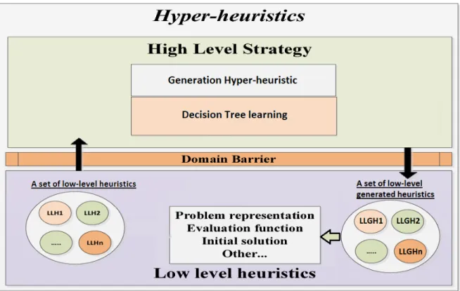
(28) CHAPTER 2. BACKGROUND. 2.2.2. 14. Generation Hyper-heuristic. Since the main development of these project is done around generation hyper-heuristics a more in-depth description of this particular model is given in this subsection. An illustration of the structure for a generation hyper-heuristic is presented in Figure 2.4. Figure 2.4: A generation hyper-heuristic structure outline for the project. This type of hyper-heuristic generates new heuristic methods using basic components of previously existing heuristic methods as illustrated in the figure above. • Based on basic components of constructive heuristics • Based on basic components of perturbative heuristics These two types of approaches for generation hyper-heuristics are based on the type of heuristics applied (perturbative or constructive) as described below: • Approach based on Constructive Heuristics As stated in the last subsection this approach focuses on building a solution incrementally. It begins with an empty solution, then generates and apply a constructive heuristic to start building a solution step by step. The hyper-heuristic is provided with a group.

(29) CHAPTER 2. BACKGROUND. 15. of general constructive heuristics and the objective is to generate the most appropriate heuristic for building part of the solution in each stage of the sequence. It is important to denote that the process of generation is finite and the size of the problem determines it. • Approach based on Perturbative Heuristics This approach begins with an initial complete solution to the problem generated randomly or through the use of constructive heuristics. Then, the objective is to improve the solution through the implementation of perturbative heuristics that are generated and applied to the problem iteratively. The process ends until meeting any stop criteria previously stated. Finally, an example of this type of generation hyper-heuristic approach is presented in [11] where a model to settle a Vehicle Routing Problem with Time Windows is developed. The model autonomously generates and selects the best heuristic for the state of the instant during the process, ending up with a comparison of two solutions from a selection and a generation hyper-heuristics perspective.. 2.3. Machine Learning. In this section, an overview of the state of the art in Machine Learning is explained, as well as a more detail description of the model classifier (Decision Tree) used for the development of this project. Machine learning in general terms is a way of programming the computer to learn from previous data. On the other hand, a more technical description could be given as stated in [47]: ”Machine learning is the process (algorithm) of estimating a model that’s true to the real-world problem with a certain probability from a dataset (or sample) generated by finite observations in a noisy environment.” There are plenty of machine learning models which are all divided into two main groups: supervised learning and unsupervised learning. The former requires labeled data to be implemented whereas the latter is designed for not labeled data.[25] Supervised learning has six frequently used models: • Logistic Regression is an effective algorithm to predict numerical data. It predicts labels by fitting a curve tendency of certain points[32] • Neural Networks is an algorithm for classifying data, which is built based on blocks of perceptrons.[42] • Decision Trees Decision trees are a structure for decision-making where each decision leads to a set of consequences or additional decisions[40].

(30) CHAPTER 2. BACKGROUND. 16. • Support Vector Machines is an algorithm that not only classifies the data but also searches for the best possible boundary. Namely, it seeks to maintain the largest distance from the data points to be classified.[36] • Deep Learning deep learning is a more complex structure of Neural Networks with hidden layers that allow it to be trained both us a Supervised learning as well as an unsupervised learning model.[34]. 2.3.1. Model Evaluation and Validation. In this subsection, a discussion of all methods for assessing and validating models in this project is carried out. First of all, it is essential to know how to quantify how good a model is for certain data, that is why metrics are required. The most popular metrics used for evaluation of Machine Learning models are: • Coefficient of determination, also called R squared or R2 score, this metric quantifies how well a logistic regression is compared to a simple curve that goes through the average of all points.[22] • F-beta Score, also known as F-score or F-measure, this metric is the harmonic mean between recall and precision. Beta weights how much importance to give between recall and precision, being 1 the value where no bias towards any of them exist. The following equation describes the outcome of scoring the models by F-beta score: Fβ = (1 + β 2 ) ·. (β 2. precision · recall · precision) + recall. (2.1). That means that whenever beta is less than 1 then the metric is weighing more the importance of precision than recall, whereas if it is higher than 1 recall gets more relevance in the metric’s score.[52] However, Recall and Precision haven’t been explained yet. Thus, Let’s begin with Recall, Recall is a property that focuses on reducing false negatives from a model’s outcome whereas Precision focuses on reducing false positives from the model’s outcome. • Receiver Operator Characteristic, Roc is a metric that assesses the relationship between the true positive rate and the false positive rate of a model given as follows: T rueP ositiveRate =. T rueP ositives T rueP ositives = (2.2) AllP ositives T rueP ositives + F alseP ositives. F alseP ositiveRate =. F alseP ositives F alseP ositives = AllN egatives T rueN egatives + F alseN egatives (2.3).

(31) CHAPTER 2. BACKGROUND. 17. Where ROC=(True Positive Rate,False Positive Rate) and its boundaries are (1,1) and (0,0) where the split or classfication of data is the worst possible whereas approaching (0,1) the classification is perfect.. Figure 2.5: Example of a ROC Curve[45] On the other hand, there are some Model Selection tools for avoiding both underfitting and overfitting for Classifiers or Regressions as shown below: • Model complexity graph, this is an error VS complexity curve degree graph, It helps to pinpoint the minimal error based on the complexity of the model. For instance, a polynomial curve can be fitted to describe certain data; if this is the case, the graph will show the error produced according to the degree of the polynomial. It is important to point out that sometimes the score is graphed instead of the error, this being the complementary value of the error. An example of a model complexity graph is shown below:. Figure 2.6: Example of a Model complexity graph[26].

(32) CHAPTER 2. BACKGROUND. 18. In the illustration above, we can see that there is a high Bias delimited area as well as a high variance area. The former means that the curve isn’t a representative model of the data which means it is underfitting whereas the latter implies that the curve has a high variance between training data points thus being non-representative of the validation data meaning that the model is overfitting. • Cross validation, in this method the entire dataset is divided into three different groups by adding a third one, the validation set, to the regular training and testing datasets. The process consists of assessing and picking the right model based on the model complexity created by just the training and validation sets.[17] • K-Fold Cross Validation, this approach tackles the problem in a different way to settle the issue that comes from cross-validation, which is that it is separated in so many groups that a significant part of the dataset is lost just for validating the problem. Therefore, what K-fold cross-validation propose is that the whole dataset should be divided k subsets where one of the k subsets is used as the test set, and the other k-1 subsets are put together to form a training set. This process is repeated k times. Then the average error across all k trials is computed. This helps prevent overfitting.[49] • Learning Curves, Learning curves is another useful tool for detecting overfitting and underfitting. It plots the error or its complementary (the score) against the number of training points. An example of the three possible ways a learning curve can have is shown below:. Figure 2.7: Examples of learning curves, in order from left to right, being the first one an underfitting curve, followed by a just right curve, and finally, an overfitting curve[39] As illustrated in the Figure above, the first graph denotes an underfitting model because of its low score in both training and testing sets even when more data is added to the model. The second graph shows a just right model because of its good score in both training and testing sets. Finally, the last graph illustrates an overfitting model due to its great score in the training set whereas its testing set does poorly, maintaining this result even with more data. • Grid Search is the most traditional tool for optimizing the hyper-parameters of a classifier or regression models, it consists of an exhaustive search between all hyper-parameters that are been assessed, it basically tries all possible combination of the hyper-parameters.

(33) CHAPTER 2. BACKGROUND. 19. introduced and selects the one that best scores. It is important to stress that it could use any cross-validation method as well as any score function for evaluating the models such as f-score, ROC, and R2.[50]. 2.3.2. Decision Tree Classifier. Since Decision Tree classifier is the machine learning method applied in this research, a more in detailed information regarding its components is illustrated in this subsection. A decision tree is basically a flowchart in which each level of the tree with the exception of the last level has test nodes (or yes/no question) of an attribute resulting in two branches splitting from the test node, thus, it is considered a binary tree. The tree consists of three types of nodes: decision nodes where tests are applied in all levels of the three but the first one and the last ones, root node where the decision tree starts, terminal nodes or leaf nodes where the final outcome of the decision tree is presented. An illustration of the decision tree with its type of nodes is shown in Figure 2.8. Figure 2.8: Decision tree’s type of nodes diagram[40]. Another relevant component of a decision tree is the measurement of impurity, which states how decision nodes will split instances making the splitting as pure as possible since fewer impurity results in a lower information gain from the testing node. There are two traditional types of impurity measurements: GINI and Entropy. The former is based on probabilistic distribution which is sensitive to changes in factors since it is a product of probabilities. The latter is also based on probability with the difference that it is a logarithmic measurement entailing less sensitiveness since the logarithm property converts the GINI product of probabilities into a sum of probabilities. It is important to denote that the measurement of impurity.

(34) CHAPTER 2. BACKGROUND. 20. is inversely proportional to the information gain. Decision tree classifier is represented as finite straight lines that divide the dataset for predicting an outcome, an illustration of this phenomena is shown in Figure 2.9. Figure 2.9: An illustrative relationship between dataset splitting for predicting outcomes and Decision Tree[43]. One of the disadvantages of decision tree classifiers is that they tend to overfit a lot, that is why a correct set up of the decision tree’s hyper-parameters is hardly required. Another possible solution to this issue is to follow a modified technique of decision trees called Random Forest. What Random Forest does is to generate a group of decision trees instead of a single tree, then each tree votes for predicting the outcome, the leaf with higher votes is the result of the random forest, this way overfitting is reduced significantly. It is called random forest due to the fact that each tree is created based on random features of the instances instead of all instances. The only issue with this approach is that it is costly to implement. [37]. 2.4. Simulation Environment. Regarding software for robotics and autonomous vehicles, there are plenty of options. However the most relevant at the moment are two combinations of software: the first one, Robot Operating System (ROS) and its native simulator GAZEBO, which are open-source software packages. The second one, Virtual Robot Experimentation Platform (V-REP) with MATLAB as API, from which V-REP grants a free license for academic purposes, while MATLAB is a payable license software. However, since there exists a high shareable software environment concerning motion planning for V-REP with MATLAB, this is the approach taken as a custom simulator for this thesis. In more detail, V-REP can be used with all remarkable OS at the moment, Windows,.

(35) CHAPTER 2. BACKGROUND. 21. Linux, MAC-OS. Also, it can be approached by six programming ways: ROS nodes, plugins, custom solutions, add-ons, embedded scripts, and API clients. The latter can be remotely implemented with different environments such as python, java, C/C++, LUA, Octave and finally MATLAB which is the chosen one for this project.[46] On the other hand, for the second phase concerning the simulation environment, a simulator from another source built in Unity has been implemented.[44] Unity is a platform mainly for the creation of games. Since the simulator’s sensor data was provided through C++ this was the language selected for developing all the algorithms required for doing the motion planning of the car.. 2.5. Related Work. Hyper-heuristics applied to motion planning of self-driving vehicles hasn’t been studied previously. However, there exist some articles related to it and some others that can help in this researching field. One of them and the most related work is about ”Motion planning for Unmanned Aerial Vehicles (UAV)” [1], followed by work on hybrid methods ”Combining selective and constructive hyper heuristics” for VRP [18]. Finally, an overview of what has been done for planning algorithms alongside with hyper-heuristics and other methods. ”Alternative Approaches to Planning” [30] We will describe each of this works in the three following sub-subsections.. 2.5.1. Motion planning for Unmanned Aerial Vehicles (UAV). This paper describes an interpolating curve planner, based on B-splines. The hyper-heuristics model applied for motion planning is a perturbative approach within a selection heuristic. The main idea is to construct a spline that best meets the constraints of the UAV while it is moving, it selects between some low-level heuristics to optimize the trajectory spline for the robot. Details of selection methodology heuristics and low-level heuristics implemented; as well as a definition of b-spline curves are explained below.. Selection heuristics Five high-level heuristics were executed by the selection model proposed in[1] as follows: • Simple Random, which selects a random low-level heuristic and applied once. • Greedy, which apply all low-level heuristics and choose the one that best performs for the instance problem..

(36) CHAPTER 2. BACKGROUND. 22. • Random Descent, it uses the same notion of Simple Random, but with the difference that it applies the random heuristic repeatedly until there is no improvement in the solution. • Choice Function, it chooses between low-level heuristics based on their performance upon a function created for the problem. Two types of strategies are used, the first one, a Straight Choice Function, picks a heuristic that improves the function. While the second one, The Ranked Choice Function, chooses a heuristic based on a ranking made from a choice function. • Reinforcement Learning, a machine learning technique as a high-level heuristic is implemented to improve the quality of low-level heuristic selection. In general terms, it is done by rewarding or punishing heuristics based on their performance.. Low-level heuristics Eight low-level heuristics were implemented for creating possible points to construct the B-spline curves. Based on the article [1], we will briefly explain these heuristics as follows: • Delete operation, a randomly selected point is deleted. • Smart Delete Operation, deletes worst point for meeting constraints. • Insert Operation, randomly inserts a point into the point list. • Smart Insert Operation, inserts the best performance point to the point list. • Update Operation, randomly replace a point with other in the point list. • Smart Update Operation, the worst fitness value point in the list is replaced by another point near the optimal path. • Smooth Turn Operation, prevents to maneuver out of the curvature radius limit of the UAV. • Shortcut Operation, fixes points that are deviated from the optimal path.. 2.5.2. Combining selective and constructive hyper heuristics for the Vehicle Routing Problem VRP. In this work, it is explained how a combination of both selection and generation heuristics can be better than each one alone. The testing was divided into two portfolios as testing environments, the first one composed of just three original construction low-level heuristics, while the second one composed by the same three heuristics but with the addition of nine new generated heuristics. The results obtained for the instances proved confirmed that the combination of both selective and generation heuristics is better than just original heuristics..

(37) CHAPTER 2. BACKGROUND. 23. For the creation of new low-level heuristics (LLHs) in this work, the approach taken was not to create a whole new LLHs but to modify original ones to get these new LLHs. The original heuristics took for this study were the following:. Clarke-Wright Savings Algorithm (CW) CW focus on savings values calculated between each city visited. It is calculated by three equations based on the distances ’d’. Da = d0i + di0 + d0j + dj0. (2.4). Db = d0i + dij + dj0. (2.5). Sij = Da − Db = di0 + d0j − dij. (2.6). From which the last equation, Sij is a parallel savings route used for determining the best path.. Mole-Jameson heuristic (MJ) This heuristic iteratively builds just one path at a time, it starts considering the largest way from the depot, and then tries to add the nearby cities not yet assigned to this route, based on two equations (4) and (5) as follows: α(i, k, j) = dik + dkj − λ ∗ dij. (2.7). β(i, k, j) = µ ∗ d0k − α(i, k, j). (2.8). where λ and µ are parameters set for influencing the values of the algorithm based on empirical assess.. Kilby algorithm (K) Kilby works similar to MJ, but with the difference that it tries to add city K into already assigned cities in a route, to seek for a lower value. The equation used in this algorithm is the following: Cri (i, k, j) = dik + dkj − dij (2.9) where ri is the current route from the set of already existing paths, if none of the existing routes can be added, then a new path is created, repeating the process until all cities are assigned.. Finally, for the creation of new heuristics, all these recently described heuristics are set into a genetic algorithm, seeking for improvements in the equations state above. After modifying each heuristics’ equations, it results in eight new heuristics for each original heuristic CW, MJ, and K. making a total of twenty-four new heuristics, from which each one is tested with a particular set of instances. To pick the best nine heuristics for adding into the portfolio of the high-level selection heuristic..

(38) CHAPTER 2. BACKGROUND. 2.5.3. 24. Alternative Approaches to Planning. As stated in [30], there are two types of planning tasks: the first one is the satisficing plan, in which we want to find a plan that meets all constraints until reaching a goal state. The second one is the optimization plan, in which we want to minimize the objective function while constructing the plan to the goal. On the other hand, as mention in the paperwork, ”no competitive planning system based on hyper-heuristics has emerged.” [30] However, there exist some portfolio-based planners such as MCTS algorithm that can be used for developing one. It is important to note that some LLH’s features that are suggested in this work as relevant for planners are: • be able to solve a satisficing planning task. • be very fast and able to find suboptimal solutions at the same time. • be diverse, but also including a copy of same algorithms with different parameters. • be using standard algorithms such as A*, IDA*, or enforced hill-climbing. • be using non-standard algorithms such as beam-stack search or symbolic search. Finally for guaranteeing the very fast LLHs’ feature as stated previously, a limit time is proposed, in a way that any LLH that exceed this constraint time will be penalized. However, the time limit is variable during execution, first at the beginning starting low and then increasing slightly on each iteration, to allow contribution of most sophisticated low-level algorithms.. 2.6. Summary. This chapter gave a general glimpse of the topics related to this project: Self-driving cars’ motion planning. Hyper-heuristics, in particular, generative high-level heuristics. Machine learning, in particular, decision tree models. The problem with motion planning is that there are plenty of heuristics that have particular disadvantages, therefore to address the issue an approach in this project is proposed through the use of generation hyper-heuristics. A hyper-heuristic is a high-level algorithm which solves a problem by either selecting low-level heuristics or generating new algorithms from a set of operators. For this thesis, a decision tree is determined to generate a heuristic that is best suited for the subproblem at hand..

(39) CHAPTER 2. BACKGROUND. 25. Finally, there is not an approach linking self-driving cars and hyper-heuristics in traditional literature. However, some projects are somehow related, such as the motion planning of Unmanned Aerial Vehicles using custom low-level heuristics. The next chapter 3 explains an outline of the solution model, followed by the methodology in chapter 4, where all the methodology followed along the thesis is explained..

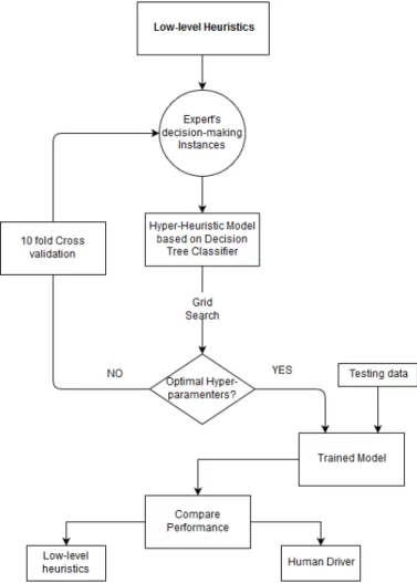
(40) Chapter 3 Solution Model In this thesis, a generation hyper-heuristic is presented. It generates a suitable heuristic from three particular low-level heuristics through a decision tree algorithm that can also be seen as a finite state machine in the simulator. An outline of the model is explained below.. Figure 3.1: Generation Hyper-heuristic Model Diagram 26.

(41) CHAPTER 3. SOLUTION MODEL. 3.1. 27. Low-level heuristics. As stated in the introduction of this document, Hyper-heuristic algorithms work over heuristics that generate solutions instead of going straight to the solution itself. Therefore, there are three low-level heuristics in the model proposed, each one has its particular approach to solve the problem. As seen in the Figure 3.1 the three low-level heuristics are of a perturbative type and are the following: • Left heuristic, attempts to get to the target location by just taking the left lane. • Center heuristic, attempts to get to the target location by just taking the center lane. • Right heuristic, attempts to get to the target location by just taking the right lane. All heuristics create a solution path through its side of the lane. This means that, for instance, the left-heuristic attempts to complete the trajectory by always going in the left lane of the highway, the same for the center heuristic and the right heuristic. Each heuristic implements a reduce speed function which makes the car going to the same velocity of the front car in its lane only if it is closer than the security distance between vehicles stated by road traffic protocols. Each heuristic generates a set of points on space that contains cartesian coordinates to locate the next targeted position as well as the velocities to set the vehicle’s speed sent to the controller afterward. The generation of the points is done through the minimum jerk trajectories MJT[29] which is a polynomial approach to interpolate points between the target destination and the instant position as well as the velocity and acceleration. This way the points sent to the controller are a smooth curve instead of an abrupt change of trajectory resulting in a minimal jerk due to the avoidance of jumps in acceleration values.. 3.2. Decision-Tree as a High-level heuristic. The high-level heuristic implemented is a machine learning technique known as the decision tree, which is in charge of learning from the low-level heuristics stated in the prior section. The Decision tree hyper-parameters and performance are assessed by the following machine learning metrics: • accuracy score, which measures the percentage of values that were correctly predicted by the model. • f1 score, also known as f-score this metric scores the performance between true and predicted values based on precision and recall..

(42) CHAPTER 3. SOLUTION MODEL. 28. • k-fold cross validation, the data set is divided into k subsets and each time, one of the k subsets is used as the test set and the other k-1 subsets are put together to form a training set. Then the average error across all k trials is computed. This helps prevent overfitting. • grid search, this technique combines all hyper-parameters of the decision tree and outputs the one that scores the best combination of hyper-parameters. This way preventing overfitting and underfitting of the model. The three hyper-parameters combined for the grid search technique are the following: 1. max depth, states the maximum depth of the tree. 2. min samples leaf, states the minimum number of samples that leaves (last nodes of the tree) must have. 3. max leaf nodes, states the maximum number of samples that leaf nodes must have at most. If a node has more than that value, another division is created. The result of the hyper-parameters for the for the optimal decision tree model are: maxdepth = 7 , minsamplesleaf = 3, and maxleaf nodes = 26.. 3.3. The Self-driving car instances. The instances used in this work are each vehicle’s state position gotten from the data of the fusion sensor. Every state has its distance to the cars on the other lanes relative to the selfdriving car. The features taken from each state are the following: • distF rontL , is the distance of the front car on the Left lane relative to the self-driving Car. • distRearL , is the distance of the rear car on the Left lane relative to the self-driving Car. • V F rontL , is the velocity of the front car on the Left lane. • V RearL , is the velocity of the rear car on the Left lane. • distF rontC , is the distance of the front car on the Center lane relative to the selfdriving Car. • distRearC , is the distance of the rear car on the Center lane relative to the self-driving Car. • V F rontC , is the velocity of the front car on the Center lane. • V RearC , is the velocity of the rear car on the Center lane..

(43) CHAPTER 3. SOLUTION MODEL. 29. • distF rontR , is the distance of the front car on the Right lane relative to the selfdriving Car. • distRearR , is the distance of the rear car on the Right lane relative to the self-driving Car. • V F rontR , is the velocity of the front car on the Right lane • V RearR , is the velocity of the rear car on the Right lane • LaneStatus, is the lane in which the car was standing when the measurement was taken • Lane decision making, is the lane-heuristic taken based on a human expert driver driving the self-driving car manually. From all of the above features, the target feature is the Lane decision making which is the selected heuristic at the instant when the state was taken. The way in which each instance was taken was by the combination of different human drivers while they were driving all data was recording each move and decision they took. Also, all its moves were filtered by only recording the ones that didn’t break any road traffic rule(incidents) and that its speed is set to the constant velocity limit, in this way we get data based on the ideal human expert driver, to assure even more a better outcome and avoid driver’s fatigue, three different drivers generated the instances instead of just one human driver, each driver drove for around twenty minutes generating more or less one thousand instances with an interval of one second per instance. The traffic rules taken into account were: not going out of the highway’s lanes, not exceeding the speed limit of 50 miles per hour or 80 kilometers per hour, and not hitting other cars or traffic signs. Another relevant information about the instances is that whenever the sensor doesn’t get data from any car on its surroundings due to them been further than its sensing range, both velocity and distance are set to 10000 for the front vehicles whereas the distance of the rear vehicles is set to 10000 but velocity to zero. A small sample of the database taken from all the instances is shown in the next Table 3.1..

(44) distFront L 97.9006 91.8467 84.9016 76.6679 11.118 11.085 10.887 11.026 10000 10000 97.744 90.971. distRear L 10000 10000 10000 10000 10000 10000 10000 10000 10000 10000 10000 10000. VRear L 0.0 0.0 0.0 0.0 0.0 0.0 0.0 0.0 0.0 0.0 0.0 0.0. distFront C distRear C VFront C 10000 10000 10000 10000 10000 10000 92.5155 10000 16.1089 83.5966 10000 16.0256 23.209 14.603 16.6749 21.992 14.377 16.6704 20.726 14.531 16.6603 20.11 14.572 16.6444 33.301 10000 15.9257 24.489 10000 15.9163 14.949 10000 15.9056 5.698 10000 15.8951. VRear C 0.0 0.0 0.0 0.0 17.6711 17.694 17.7124 17.7165 0.0 0.0 0.0 0.0. distFront R distRear R VFront R 10000 10000 10000 10000 10000 10000 10000 10000 10000 10000 10000 10000 10000 10000 10000 10000 10000 10000 10000 10000 10000 10000 10000 10000 45.313 10000 17.3691 36.832 10000 17.3634 29.346 10000 17.3545 20.284 10000 17.3399. VRear R 0.0 0.0 0.0 0.0 0.0 0.0 0.0 0.0 0.0 0.0 0.0 0.0. Lane status Lane decision making 2 2 2 2 2 2 2 2 2 3 2 3 2 3 2 3 2 1 2 1 2 1 2 1. Table 3.1: A small sample of data taken from instances generated by human drivers. VFront L 17.9013 17.4982 17.2537 17.1158 17.6367 17.6365 17.6349 17.6354 10000 10000 19.169 18.5711. CHAPTER 3. SOLUTION MODEL 30.

(45) CHAPTER 3. SOLUTION MODEL. 3.4. 31. Summary. This chapter reviewed an overview of the solution model, which is explained in three general sections. Low-level heuristic section, where an explanation of the heuristics implemented in the project is held. High-level heuristic section, where an overview of the tools and the result for the hyper-parameters that the decision tree obtained for selecting between lowlevel heuristics was explained. The instances section, where the methodology of getting the instances for the problem was discussed. The whole remaining process of the methodology taken for getting to the model shown in this chapter is going to be explained in chapter 4 Methodology..