Doctoral Thesis
Structural optimization of steel jackets for
offshore wind turbines considering dynamic
response and fatigue constraints
Iv´
an Couceiro Aguiar
Supervisors:
Dr. Jos´
e Par´ıs L´
opez
Dr. Ferm´ın Navarrina Mart´ınez
It takes time for society to digest changes, but we are changing. We can not deny climate change anymore and, as a species, we have come to realize there is an urgent need to change our energy generation habits. They have changed indeed and, in the last decades, renewable energies have clearly colored the picture of energy sources. Particularly, wind energy is called to be one of the most valuable cards in the hand of renewable energies in the near future. However, the current trend, and target of this thesis, are not the typical wind turbines installed inland. In the last years, the preferred location for the placement of wind farms has traveled, or we better say sailed from land to the seas, seeking for higher efficiency and exploitation of wind’s potential. Even though there are reasons to carry wind turbines offshore, the trip is neither easy nor low-cost and implies the analysis and design of new substructures to bear the weight of the turbines. Those substructures are called jackets.
This thesis defines a procedure of analysis of the dynamic behavior of offshore wind turbines supported by jackets. Upon that analysis, a structural optimization problem is defined and solved using mathematical and numerical optimization techniques. The goal is to reduce the amount of material needed to manufacture the jackets and therefore reduce the investment of offshore wind turbine structures and consequently the indirect cost of energy production.
The structural model is based on a non-linear dynamic analysis of three dimensional framed structures for fully coupled offshore wind turbines considering the rotation of the blades. Special care is taken in the description of the environmental loading condi-tions. Wind and wave actions and forces on the elements of the structure are thoroughly modeled. One of the most decisive aspects in the design of offshore structures is fatigue in steel elements arising from cyclic loads. In this thesis fatigue damage is assessed in terms of S-N curves by means of the Palmgren-Miner rule and using the Rainflow algorithm for counting stress cycles. Long-term fatigue damage in the joints of the jack-ets is accurately estimated from the damage computed for short-term computational simulations.
The optimization model is presented as a weight minimization of the steel jacket under Ultimate Limit Stress, Fatigue Limit State and frequency constraints. Cross-sections of the tubular elements and bottom and top widths of the jacket are chosen as design variables to perform a simultaneous shape and size optimization while preserving the straight alignment of the legs. The optimization is addressed using Sequential Linear Programming which requires a first order sensitivity analysis. The sensitivities are obtained through Direct Differentiation and analytic derivatives except for the fatigue damage constraint since it lacks analytic derivative. The sensitivity core of the computational code constitutes an extremely expensive part in terms of CPU time and storage.
Contents I
List of Figures V
List of Tables IX
Prologue XI
1 Introduction 1
1.1. Background . . . 2
1.2. Review. . . 7
1.3. Motivation . . . 9
1.4. Objective . . . 10
1.5. Organization . . . 10
2 Mathematical and numerical modeling 13 2.1. Introduction. . . 13
2.2. Previous considerations and hypotheses . . . 14
2.3. Structural model . . . 15
2.3.1. Global and local coordinate systems . . . 15
2.3.2. Stiffness matrix . . . 18
2.3.3. Mass matrix . . . 23
2.3.4. Damping matrix . . . 25
2.4. Loading conditions and loads modelization. . . 25
2.4.1. Gravity . . . 26
2.4.2. Buoyancy . . . 27
2.4.3. Wind . . . 28
2.4.4. Waves . . . 33
2.4.5. Distributed loads treatment . . . 38
2.5. Dynamic analysis . . . 39
2.5.1. Natural frequencies and modes of vibration . . . 39
2.5.2. Equation of motion and time integration. . . 41
2.6.2. Hot Spots . . . 51
2.6.3. Counting algorithms . . . 52
2.6.4. Fatigue life assessment . . . 53
2.7. Summary and conclusions . . . 57
3 Optimization problem 59 3.1. Introduction. . . 59
3.2. Definition of the optimization problem . . . 60
3.2.1. Objective function . . . 61
3.2.2. Structural and design constraints . . . 61
3.2.3. Design variables . . . 69
3.3. Time-dependent constraints handling . . . 71
3.3.1. Short review of time-dependent constraints treatment . . . 71
3.3.2. Constraint aggregation functions and proposed method . . . 73
3.4. Summary and conclusions . . . 75
4 Sensitivity analysis 77 4.1. Introduction. . . 77
4.2. Notation . . . 77
4.3. Differentiation method . . . 79
4.4. Elemental derivatives. . . 81
4.4.1. Mechanical properties derivatives . . . 82
4.4.2. Length derivative. . . 82
4.4.3. Structural matrices derivatives . . . 85
4.5. Constraints sensitivities . . . 89
4.5.1. Constraints sensitivities handling . . . 89
4.5.2. ULS constraints derivatives . . . 91
4.5.3. Differentiation of the dynamic equation . . . 91
4.5.4. External forces derivatives. . . 92
4.5.5. Aggregated constraints derivatives . . . 99
4.5.6. FLS constraints sensitivities. . . 100
4.5.7. Frequency constraints sensitivities . . . 104
4.6. Objective function sensitivity . . . 105
4.7. Summary and conclusions . . . 106
5 Optimization method 107 5.1. Introduction. . . 107
5.2. Optimization algorithms and offshore engineering . . . 108
5.3. Optimization algorithm . . . 111
5.3.1. Sequential Linear Programming. . . 111
5.4. Optimization methodology and numerical implementation . . . 117
5.5. Summary and conclusions . . . 120
6 Application examples 121 6.1. Introduction. . . 121
6.2. Model description. . . 122
6.2.1. Jacket . . . 125
6.3. Performance and efficiency. . . 126
6.4. Optimization parameters. . . 127
6.4.1. Moving limits for the SLP Method . . . 128
6.4.2. Activation limit. . . 129
6.4.3. Design variables influence . . . 130
6.5. Rotation influence . . . 131
6.5.1. Initial design . . . 132
6.5.2. Optimization process. . . 133
6.5.3. Optimum design . . . 135
6.6. Approximation of real environmental conditions. . . 136
6.7. Changes in the design . . . 139
6.7.1. Number of X bracing blocks . . . 139
6.7.2. Number of X bracing blocks avoiding complex joints . . . 145
6.7.3. Horizontal braces . . . 149
6.8. Summary and conclusions . . . 151
7 Remarks, conclusions and further developments 153 7.1. Introduction. . . 153
7.2. Remarks and conclusions . . . 153
7.2.1. Structural model . . . 153
7.2.2. Optimization model . . . 154
7.2.3. Optimization results . . . 155
7.3. Further developments . . . 156
7.3.1. Structural model . . . 156
7.3.2. Optimization approach. . . 158
7.3.3. Others . . . 159
A Stress concentration factors for fatigue life design 161 A.1. Introduction. . . 161
A.2. Previous considerations and hypothesis. . . 162
A.3. Geometrical properties . . . 164
A.4. SCFs formulas. . . 164
A.4.1. T/Y joints . . . 165
B Constraints Sensitivities 169
B.1. Introduction. . . 169
B.2. Ultimate Limit State constraints . . . 170
B.2.1. Axial tension and bending without hydrostatic pressure . . . 170
B.2.2. Axial compression and bending without hydrostatic pressure . . 171
B.2.3. Axial tension and bending with hydrostatic pressure . . . 173
B.2.4. Axial compression and bending with hydrostatic pressure . . . . 175
B.2.5. Shear, bending and torsional moment . . . 177
B.2.6. Hoop Buckling . . . 179
B.3. Fatigue Limit State constraints . . . 179
B.3.1. Derivative of the geometrical parameters of the joint . . . 180
B.3.2. Derivative of the dimensional constraints . . . 181
B.3.3. SCFs sensitivities for T/Y joints . . . 181
B.3.4. SCFs sensitivities for X joints . . . 183
B.3.5. SCFs sensitivities for K joints . . . 184
C Extended summary in Spanish 189
D Extended summary in Galician 197
1.1. Traditional windmill and modern wind turbines . . . 2
1.2. Onshore vs Offshore wind farms . . . 3
1.3. Wind power trend in the EU . . . 4
1.4. Main offshore wind turbines substructure concepts . . . 5
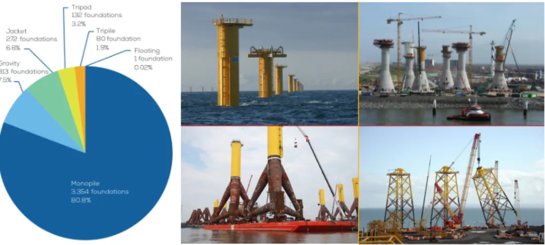
1.5. Substructures types in EU offshore wind farms . . . 6
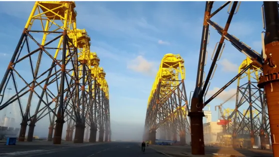
1.6. Wikinger jackets ready to be shipped in Denmark . . . 7
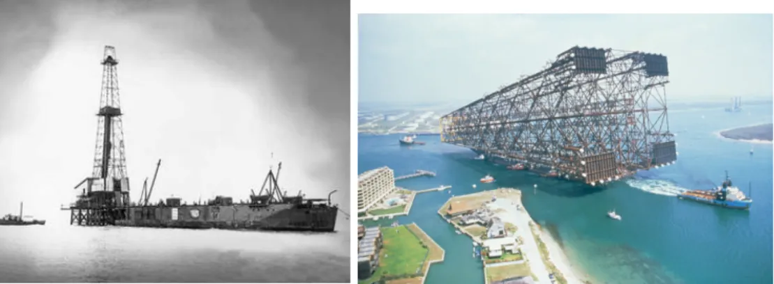
1.7. First offshore jacket structures . . . 8
1.8. Conceptual estimated cost vs depths for OWT substructures and typical cost distribution comparison in Onshore and Offshore windfarms . . . 10
1.9. Wikinger jackets installed . . . 11
2.1. Global and local axes of a structural member . . . 15
2.2. Roll angle of the member . . . 17
2.3. First and second natural vibration modes with and without the additional local axes formulation . . . 19
2.4. Global axes displacements . . . 19
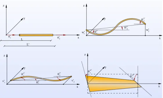
2.5. Local axes displacements . . . 20
2.6. Local movements and strains of an element . . . 21
2.7. Jacket launching operation . . . 26
2.8. Marine growth over tubular elements . . . 27
2.9. Conditions for the cross sections of the jacket . . . 28
2.10. Stream-tube and wind velocity profiles across the actuator disc . . . 29
2.11. Velocities and forces on the blade element . . . 30
2.12. Torque and thrust comparison with the reference model . . . 32
2.13. Tower dam effect . . . 34
2.14. Wave theories and kinematics . . . 35
2.15. Comparison of natural frequencies from existing codes and current work . . 41
2.16. First natural frequencies and modes of the OC4 jacket computed . . . 41
2.17. Fore-aft shear at mudline . . . 43
2.18. Computing time for the steady and rotating case for different time steps . . 46
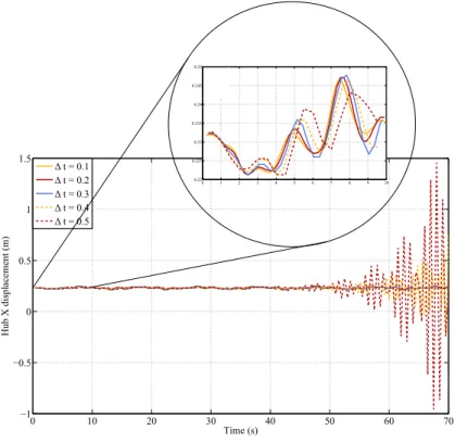
2.19. Hub displacement in X direction . . . 47
2.23. Rainflow counting process . . . 54
2.24. Calculated and estimated damage 1 . . . 56
2.25. Calculated and estimated damage 2 . . . 56
3.1. Decision tree for ULS constraints . . . 66
3.2. Wave scatter diagram . . . 67
3.3. Campbell diagram and 1P and 2P frequency bands . . . 69
3.4. Optimization design variables . . . 71
3.5. ρinfluence with 10% constraints active. . . 75
3.6. ρinfluence allowing 2% violation of the constraints . . . 75
4.1. General data flow in an analysis and design optimization numerical imple-mentation . . . 79
4.2. Variation of the coordinates with respect to the geometrical design variables 83 4.3. Z coordinate of the intersection in X joints . . . 84
4.4. Computing time for the steady and rotating case for different time steps including the sensitivity analysis with 22 design variables . . . 92
4.5. Wave direction and global axes . . . 95
4.6. Number of stress blocks for each hot-spot in a base design and a design modifying the design variables . . . 101
4.7. Initial and reversal points for two different cycles of the same amplitude counted by the rainflow . . . 101
4.8. Flowchart comparison between sensitivity analysis approaches for fatigue damage . . . 102
5.1. General simplified scheme of optimization methods . . . 108
5.2. Linearization of the objective function and constraints . . . 112
5.3. Moving limits in the SLP method. . . 113
5.4. Numerical implementation scheme . . . 118
6.1. Rotor-nacelle assembly model . . . 124
6.2. Examples of transition pieces . . . 124
6.3. Transition piece modeling options. . . 125
6.4. OC4 jacket geometry. . . 126
6.5. Optimization evolution for different activation limits . . . 130
6.6. Comparison between shape and size optimization performed separately. . . 131
6.7. Comparison of displacements between the non-rotating and the rotating case132 6.8. Stresses at leg 1 and hot-spot 1 in the non-rotating and rotating case. . . . 133
6.9. Evolution of the objective function and the number of active constraints for the non-rotating and the rotating case . . . 134
6.12. Evolution of the design during the optimization process . . . 139
6.13. Design variables optimization process . . . 140
6.14. Design variations by adding or removing X bracing blocks on the basic OC4 jacket . . . 142
6.15. Evolution of the objective function for the modified designs and optimum geometry and sections . . . 143
6.16. First natural frequency of the designs and evolution of the geometrical de-sign variables . . . 144
6.17. Feasible region for dimensional constraints . . . 145
6.18. Conical transition between tubular sections and changes in thickness . . . . 146
6.19. Section transition location avoiding the generation of complex joints . . . . 146
6.20. Evolution of the objective function for the modified designs with interme-diate joints and optimum geometry and sections . . . 148
6.21. Displacement in the global X axis of the head center of the optimized jackets and comparison for the 3XM design with and without considering the tower dam effect . . . 149
6.22. Evolution of the objective function for the modified designs with interme-diate joints and horizontal braces, and optimum geometry and sections. . . 150
7.1. Soil-structure interaction model and dynamic p−y curves . . . 157
7.2. Large deformations of wind turbine blades . . . 158
7.3. Height of jacket’s blocks as design variables schematics. . . 159
A.1. Types of tubular joints. . . 162
A.2. Joint classiffication according to forces balance . . . 162
A.3. Geometrical definition for tubular joints . . . 164
A.4. Geometrical definition of an X joint . . . 166
6.1. Cross-sectional properties of the tower elements . . . 123
6.2. Cross sections of the members. . . 126
6.3. Combinations of cross-sections circumstances. . . 126
6.4. Material properties. . . 126
6.5. Additional masses. . . 126
6.6. Optimized results for different moving limits (ML). . . 129
6.7. Ratio between the rotating and non-rotating total fatigue damage at design life for the 4 legs of the jacket at the third level. . . 133
6.8. Design variables comparison between the rotating and the non-rotating model (dimensions in meters for diameters and widths and millimeters for thicknesses).. . . 136
6.9. Description of the lumped load cases for ULS and FLS. . . 138
6.10. Height of the X bracing blocks in the modified designs.. . . 141
6.11. Weight, iterations, active constraints and shape design variables at the op-timum changing the height of the blocks. . . 141
6.12. Diameter in meters of the designs changing the height of the blocks. . . 143
6.13. Thickness in millimeters of the designs changing the height of the blocks. . 143
6.14. Weight, iterations, active constraints and shape design variables at the op-timum changing the location of the transition between sections.. . . 147
6.15. Diameter in meters of the designs changing the location of the transition between sections. . . 147
6.16. Thickness in millimeters of the designs changing the location of the transi-tion between sectransi-tions. . . 147
6.17. Diameter in meters of the designs adding horizontal braces. . . 150
6.18. Thickness in millimeters of the designs adding horizontal braces. . . 150
“Est´ais esperando mis palabras. Me conoc´eis bien y sab´eis que soy incapaz de permanecer en silencio. Callar, a veces, significa mentir, porque el sliencio puede interpretarse como aquiescencia.”
Miguel de Unamuno
Not many accept the challenge of reading a whole PhD thesis. Some will do it for pleasure, some will be forced to do so (sorry). Probably, most of them will read just the parts they are particularly interested in, the mathematical description, the numerical approach, the results (only the pictures)... But, some will tragically, yet inevitably, leave their bookmarks forever in the introduction chapter.
So, I am going to do my best and try to lure you towards reading the rest of the document on the first pages.
Chapter
1
Introduction
“A man’s true honour cannot be outraged by what he suffers, but only and alone by what he does; for there is no saying what may befall any one of us”
Arthur Schopenhauer, The art of being right.
O
nce upon a time, a man encountered a river in his path. Since he was granted the gift of rational thinking, he asked himself three questions before even start doing anything. The first question, that was already answered by its inborn determination, was: What am I doing?, to which he replied relentlessly: I’mcrossing this river. The second question, which is the most meaningful, was: Why am I
doing it?, and the third: How do I do it?...
I would like to think those three questions,What?, Why? andHow?, not partic-ularly in that order, are absolutely necessary for any activity claiming to be called rational. While the frontier between them is sometimes blurred and we could argue for days about the extent of each question and yet never reach an understanding; by responding to them we are undoubtedly revealing our purpose, motive and the means we plan to use to reach our end.
This chapter is about answering those questions. More precisely this chapter deals with the first two questions, and the remaining219pages of this document are a hopeful attempt of response to the third.
1.1.
Background
It takes time for society to digest changes, but we are changing. We can not deny climate change anymore and, as a species, we have come to realize there is an urgent need to change our energy generation habits.
They have changed indeed and, in the last decade, renewable energies have clearly colored the picture of energy sources where fossil fuels, nuclear energy and natural gas were the primary elements. Particularly, energy extracted from the wind will be one of the most valuable cards in the hand of renewable energies in the near future.
The use of the wind resource is not new whatsoever. Windmills are undoubtedly the ancestors of modern wind turbines. They are said to be nearly 3000 years old although, the first reliable record is from 644 A.D. Regardless of their age and origin, they were an economic stilt during the Early and Late modern period1.
Figure 1.1. Traditional windmill (Goliath 1897) and modern wind turbines in Eemshaven, Netherlands.
The fact is, wind power is now the main bet in terms of changing our energy resources. The worldwide power generation capacity from wind has grown in the last
1A detailed and enjoyable historical background on windmills and windwheels that can be read in
decade from less than 100 GW to almost 500 GW in 2016 2. Particularly in the European Union (EU) the installed wind power capacity reached in 2016 the second largest form of power generation capacity, overtaking coal3. Figure 1.3shows some of
the main indicators of the wind energy evolution in the EU since 2005.
However, the current trend, and target of this thesis, are not the typical wind turbines installed inland. In the last years, the preferred location for the placement of wind farms has traveled, or we better say sailed from land to the seas. In the field’s jargon, one is called onshore wind and the other offshore wind (1.2).
(a) Onshore wind farm (source: inhabitat). (b) Offshore wind farm (source: Siemens).
Figure 1.2. Onshore vs Offshore wind farms.
Offshore wind is not the only card alone in the deck, it is half of a bigger strategy to squeeze the raw energy of the oceans: Offshore Renewable Energy (OWE). The other half is known as ocean energy which is the extraction of energy from waves, currents, tides, etc. There are even combined proposals to merge both strategies in singular structures or devices [Karimirad,2014;P´erez-Collazo et al.,2015].
Even though there are reasons to carry wind turbines offshore, the trip is neither easy nor low-cost. The main justification to plant the seeds of wind energy harvesting out in the seas is simple: wind is steadier and stronger offshore. The latter means higher efficiency and exploitation of wind’s potential. Nevertheless, the drawbacks are easy to see. We are severely separating generation from consumption, so there is a need to wire new subsea transmission lines and built both, offshore and onshore substations. Also, the erection of wind turbines out in the middle of the sea means the development of new methods to sustain or hold their weight. While the tower, nacelle and blades remain similar to their onshore cousins, we need some method to support the whole structural system below the tower.
There are numerous types and concepts of substructures as supports of Offshore Wind Turbines (OWT). Each of them is particularly suitable or viable at certain ranges of depths. Even though the depth frontiers for each technology are not firmly
20050 2006 2007 2008 2009 2010 2011 2012 2013 2014 2015 2016 50
100 150
Cumulative installations (GW)
onshore
offshore
a) c)
d)
e) b)
Figure 1.3. Wind power trend in the EU. a)Primary production of energy from wind 2005, 1000 tonnes of oil equivalent. b)Primary production of energy from wind 2015, 100 tonnes of oil equivalent. c)Shares ins installed capacity 2005/2016 from energy sources. d)Onshore and offshore cumulative installed capacity 2005-2016 in GW. e)New asset
in wind energy 2010-2016 in onshore and offshore. Sources: Eurostat, WindEurope,
lished, there is a wide gap between two conceptually different substructure approaches: bottom supported and floating.
While floating substructure concepts are mostly drafts and prototypes, bottom sup-ported structures are solidly endorsed by engineering experience, in fact, they come from the old offshore oil and gas platforms substructures4. Additionally, bottom sup-ported structures can be divided in bottom fixed and compliant. The former behave as a rigid body and must resist the full dynamic forces and the latter are designed to deflect with the action of environmental loads and reduce the dynamic force suf-fered. Either way, bottom supported OWT build a structure that connects the base of the tower with the sea bottom and floating OWT do not. Figure 1.4draws the most common types of substructures arranged by recommended depth suitability.
monopile gravity
based tripod jacket
compliant
towers stabilizedballast
mooring line stabilized
buoyancy stabilized
+depth
Bottom fixed Floating
Figure 1.4. Main offshore wind turbines substructure concepts.
Among the common substructures pictured in figure1.4, there is one that overcomes the rest in terms of number of units actually installed: monopiles. Monopiles are simple steel pipes ranging 2.5-6.0 m of diameter, hammered into the seabed and allowing straightforward calculation, fabrication and transport. However, monopiles are highly limited. The limit for them is said to be at 25-30 m deep and bearing 5-6 MW turbines, and that using 6.0 m diameter tubes which generate quite heavy structures.
In the deployment of offshore technology, the current challenge are the intermediate water depths 30-60 m, for which the developers have traditionally preferred the jacket type foundations. Jackets are 3D framed rigid structures formed by steel tubes of 0.5-2.0 m of diameter and around 500-600 t of weight. Most of the offshore wind farms up to the date are supported by monopiles, representing in 2016 more than 80% of OWT substructures while jackets only a 6.6% in Europe. One of the key factors is that, the share increase for Gravity based and tripod foundations already stopped in 2016 and jackets are just now starting to rise in new projects and future plans. Most of the actual
projects under construction or already authorized to begin that tackle intermediate depths and big wind turbines of 7-8 MW use jacket foundations: Aberdeen, Beatrice, East Anglia 1, Hornsea Project, Neart na Gaoithe, Thanet Extension (UK projects with more than 600 wind turbines of 7 and 8 MW and depths ranging 30-56 m); Borkum Riffgrund 2, Wikinger (Germany projects with almost 100 turbines in depths up to 40 m); Nissum Bredning Vind (Denmark); ´Eolien en mer de la Baie de Saint-Brieuc (France, 62 8MW turbines in 28-36m depths); Longyuan Jiangsu Dafeng (China, 80 turbines); Tamra, Southwest (South Korea, 30 3 MW turbines up to 20 meters deep); Block Island Project5, Fisherman’s Atlantic City Windfarm Phase I, Coastal Virginia
(USA windfarms in depths of 20-40 meters).
Figure 1.5. Share of substructures types in EU offshore wind farms in 2016 (source:
WindEurope) and examples of most used bottom-fixed structures.
So the trend is clear, jackets are developers’ weapon that will help them face the challenge of conquer deeper waters and more powerful turbines.
Yet, there are many engineering and technological features of jackets’ analysis and design subject to uncertainties or unresolved. The mere structural analysis of the jackets and the definition and fulfillment of the particular strength requirements is a cumbersome process. Some of the physical phenomena critical to the design life of the structure, such as fatigue in steel, are hard to assess accurately. The impact of the in-place environmental conditions implies the definition of an unmanageable number of load cases which also generate an even greater amount of structural output data.
Above those issues arises the question if the designs of the steel jackets could be improved and optimized in terms of reducing the investment cost of the structure while meeting the same structural and strength requisites.
5The Block Island Project was the first USA offshore wind farm, located near Rhode Island with
Figure 1.6. Wikinger jackets ready to be shipped in Denmark (Source: Bladt Industries).
1.2.
Review
Although jacket structures for offshore wind turbines are relatively new, marine bottom-fixed steel structures exist from early 1900s. The Kerr-McGee drilling platform in figure 1.7a, known as Kermac Rig No. 16, was the first offshore rig in the Gulf of Mexico that was out of sight of land. From that very first milestone in 1947 to the 50.000 tonnes Bullwinkle colossal placed also in the Gulf of Mexico only 41 years passed. This fact may be seen as a reflection of how quickly the development for offshore petroleum structures grew based on strong economic interest. History is being repeated now but luckily for us the sought resource is wind instead of oil.
Even though mathematical optimization techniques, and particularly structural op-timization, is older than these developments, the actual industry has always been reluc-tant to include them in the design process. Moreover, the advances in the optimization of offshore structures are still far from matured as we are yet in the phase when several works begin to appear without a common approach. Even the mere modelization of offshore wind turbines is still unclear and subjected to many uncertainties, the first world offshore wind farm dates 1991 and the first one to use jacket substructures was the Beatrice Demonstration in 2007.
(a) Kermac Rig 16 from New Orleans Times-Picayune.
(b) Shell’s Bullwinkle Jacket.
Figure 1.7. First offshore jacket structures.
One of the first works noteworthy is [Yoshida, 2006], even though it is focused on an onshore turbine, they performed an optimization of the turbine tower in the time domain considering extreme and fatigue constraints. In [Karadeniz et al., 2010], a reliability-based optimization is proposed to account for uncertainties in the design of the jackets. The probabilistic constraints are based in extreme conditions but authors mention that the formulation can be extended to take into account fatigue probabilis-tic design. [Yan et al., 2010] performed an optimization of a platform jacket based on the ANSYS analysis and optimization toolbox under extreme loading. Their work considered the dimensions of the deck and the cross-sections of the main jacket’s piles as design variables. [King et al.,2013] compared the influence in the design optimiza-tion of considering either superposioptimiza-tion approaches or partially integrated and fully integrated models using Damage Equivalent Loads (DEL). In [Nasseri et al.,2014], au-thors optimize another jacket for a platform using a genetic algorithm with the weight of the jacket as objective function and diameter and thickness of the tubular members as variables under extreme loading. They use directional environmental data for the load cases.
Particularly, the Norwegian University of Science and Technology has been ex-tremely active in this field in the past years. Their progress is reflected in many scientific publications in journals and conferences as well as the ABYSS project funded by The Danish Council for Strategic Research [Zwick et al., 2012; Chew et al., 2013;
Muskulus & Schafhirt,2014;Schafhirt et al.,2014,2016;Chew et al.,2016]. A common feature of those works is the optimization only of the cross-sections of the members of the jacket structures and the utilization of the FEDEM software either for the dy-namic analysis or for load calculations. The use of the rainflow counting algorithm is also extended in all works.
modifying the dimensions of the elements based on which one is the farthest from its behavioral limit. In [Chew et al., 2013] a comparison between 3-legged and 4-legged jackets is carried out with an optimization of the 3-legged version. DELs are used and the stability of the members is incorporated as a check out of the optimization loop. Later their work expanded to a gradient based optimization with analytical sen-sitivities of the constraints and the use of Sequential Quadratic Programming (SQP) method of MATLAB [Chew et al.,2016]. The time-dependent constraints are treated with the worst-case approach which considers only the maximum of the constraint in time without regard of whether that maximum can appear at another time point in the next optimization iteration. In [Schafhirt et al.,2014] authors based their analysis in 30 seconds simulations using Genetic Algorithm for the optimization and also for analysis shortcuts. In later works a local optimization approach is proposed in which it is assumed that changes in the properties of the members do not affect the response of the structure [Schafhirt et al.,2016]. This is assumed valid for simultaneous changes in all members of the structure which are optimized individually.
It is also worth mention the work developed in [Oest et al., 2017]. Analytical gradients are used for the optimization. However, the loads are considered independent of the design variables and a quasi-static structural analysis is performed to evaluate the behavior of the structure. The optimization is carried out using the Sequential Linear Programming (SLP) method implemented in the CPLEX optimizer of ILOG-IBM. This is one of the most complete works in optimization of offshore jacket structures up to date, together with [Chew et al.,2016].
1.3.
Motivation
Question Why? is actually a chain of questions that have already been answered in the background section. For example, questionsWhy wind?, why offshore? or why jackets? have already been addressed in this dissertation. I would also like to think we have reached a point where there is no need to answer why renewable sources?
But, the final question ofWhy optimize jackets? is still unanswered.
The fact is, jackets are becoming the preferred support structure to reach deeper waters and bear more powerful turbines. So presumably, there is going to be countless jackets across the seas in the near future. Thus, those jackets, they better be perfectly designed so we do not end up unnecessarily wasting useful resources. Moreover, jackets represent a significant part of the budget in the deployment of an offshore wind farm and, the deeper the waters the higher the cost of the structure (figure 1.8). It is also noteworthy the few works bold enough to face the optimization of offshore jackets, not only because the novelty of the problem but because how hard it is to approach and solve accurately and efficiently.
Estimated cost
Depth (m)
0 20 40 60 80 100 120 140
Gravity, monopiles Tripods, jackets, compliant Floating
shallow
water transitionalwater deep water Turbine System
Foundation miscellaneous Grid connection
Transmission
Array cabling Others Turbine System Foundation Onshore cost distribution Offshore cost distribution
Figure 1.8. Conceptual estimated cost vs depths for OWT substructures (Adapted from:
[Musial et al.,2006] and typical cost distribution comparison in Onshore and Offshore
windfarms (Data Source: WindEurope)
1.4.
Objective
What this thesis approaches is the description of a procedure of analysis of the dynamic behavior of offshore wind turbines supported by jackets. Upon that analysis, a structural optimization problem is defined and solved using mathematical and nu-merical optimization techniques. The goal is to reduce the amount of material needed to manufacture the jackets and therefore reduce the investment of OWT substructures and consequently the indirect cost of energy production.
In summary, the main objective of this thesis is the development of a structural optimization methodology to find the optimum designs of fixed steel jackets for offshore wind turbines.
Additionally, the main goal can be divided in intermediate or second level objectives that, although is soon to discussed them here, can be summarized as:
• Set the characteristics of the dynamic structural analysis of a fully-coupled off-shore wind turbine and solve the time dependent response of the structure.
• Define a procedure to asses or estimate the fatigue damage during the whole life of the structure without the need of too long numerical simulations.
• Define an optimization problem in accordance to the structural requisites.
• Make the optimization problem manageable.
• Solve the optimization problem proposed and test its robustness in numerical examples.
1.5.
Organization
Now comes the hard part. The part that requires 3 years of devoted work and219
• Chapter 1: The present chapter serves as introduction to the matter, gives a little background on the subject, sets the objective, the motivation and the outline of the document.
• Chapter 2: It is by far the longest chapter of the thesis. It contains the description of how the structural model is built, the modelization of the environmental loads, the numerical techniques used to solve the structural dynamic problem and the definition of the method for fatigue life assessment.
• Chapter 3: It defines step by step all the elements that conform the optimization problem proposed for jackets of offshore wind turbines and how can it be handled efficiently.
• Chapter 4: It describes the first order sensitivity analysis carried out which is necessary to solve the optimization problem proposed.
• Chapter 5: It defines the optimization methodology and describes the algorithm utilized to achieve the optimum designs of the jackets.
• Chapter 6: This chapter presents the application of the optimization method to several jacket examples with emphasis in the explanation of the optimum designs reached.
• Chapter 7: Finally, a few conclusions are drawn and some key topics are marked as interesting for future research developments.
There are two additional appendices as support information considered useful but not worthy of the space they would take within the main chapters.
Chapter
2
Mathematical and numerical
modeling
“Eventually I concluded that language was bigger than the universe, that it was possible to talk about things in the same sentence which could not both be found in the real world. The real world might conceivably contain some object which had never so far been moved, and it might contain a force that had never successfully been resisted, but the question of whether the object was really immovable could only be known if all possible forces had been tried on it and left it unmoved. So the matter could be resolved by trying out the hitherto irresistible force on the hitherto immovable object to see what happened. Either the object would move or it wouldn’t, which would tell us only that either the hitherto immovable object was not in fact immovable, or that the hitherto irresistible force was in fact resistible”
Mike Alder
2.1.
Introduction
This might be the longest, densest and most heterogeneous chapter of this thesis. Even though it is not about optimization, and it may not be appropriate to talk about it here, this thesis certainly is about optimization and so, everything in this document is somehow related to it.
one can only begin to scratch the surface of those deep expertise areas in an effort to extract the necessary pieces, and this chapter is all about that.
This chapter deals with: how the whole structure; including the jacket, the tower, the rotor-nacelle assembly and the blades, is modeled; how the different nature loads affect the structure, and how they are computationally represented and applied; how is this all merged to replicate the behavior of the structure dynamically as realistic and accurate as possible; and how do we fight with a phenomenon not yet fully understood as fatigue.
And there it is the reason why this chapter is the longest, densest and by far the most heterogeneous.
2.2.
Previous considerations and hypotheses
Particular hypotheses are made and described in each of the forthcoming sections, however some bigger picture assumptions are given here since it would be confusing to justify them later.
One of the first and unsettled dilemmas was: Could the tubular members of the jacket be considered beams or given their diameter to length ratio and their thickness do they need to be considered as shells? From a local approach, each tubular element conforming the jacket is indeed a shell.
However, calculating the natural frequencies of individual elements it can be seen that the first vibration modes are beam type modes. Moreover, when combining all members in the whole jacket structure, the global natural vibration of the structure is dominated by beam modes. Thus, the dynamic behavior of the jacket structure can be modeled with beam elements accurately enough. Additionally, the optimization prob-lem proposed in this thesis using shell eprob-lements instead of beam eprob-lements would grow in a size unmanageable for the current computational resources and lacking justification given the reasonable accuracy of the beam elements model.
There are three types of connections: hinged, rigid and semi-rigid. While the joints of the jacket structures are design and built as rigid as possible it might be more precise to take them for semi-rigid, although it would imply to introduce a stiffness coefficient for the rotation of each joint around each axis reflecting the actual rotational restraint of the node. Nevertheless, the gain in accuracy can be easily lost if those coefficients are not accurately obtained. Also, even though the joints are not perfectly built, the rigid connection model gives a proper representation of the actual behavior of the union.
2.3.
Structural model
Previous to the structural analysis, all the details and characteristics that define the numerical model which represents the actual structure, and its particularities, needs to be settled. The following describes step by step how the numerical model of the structure is built.
2.3.1.
Global and local coordinate systems
Three dimensional space frames and their structural analysis call for a definition of two different coordinate systems. The overall geometry of the space frame, loads, displacements and restraints are described with reference to a global right-handed co-ordinate systemXY Z (defined by the unit vectorseeeX,eeeY andeeeZ). With three
coor-dinates for each joint there are 6 degrees of freedom per joint, three displacements and three rotations. The solution of the dynamic equations of motion is as well performed in the global reference system.
However, for each member, a local reference frame (xyz defined by the unit vectors
eeex,eeey andeeez) is established to be able to derive the stiffness and mass relations for
each element. We also need the transformation matrix that relates the coordinates of both systems for each element [Kassimali,2012].
Z
Y
X
x y z
GLOBAL AXIS
local axis
1
2
Figure 2.1. Global and local axes of a structural member.
the globalZ axis and the localxaxis. This leads to a vertical xz plane and a parallel to the horizontaly axis.
Let the direction of the unit vectoreeex of the localxaxis be defined by its direction
cosines denoted byr:
rxX= cos (θxX) =
Then the direction of they axis is defined as:
eeey =eeeZ ×eeex= det
Finally, the z axis is defined as the cross product between the x axis and the normalizedy axis:
Thereby, the transformation matrix from global to local axes is:
R
In addition, there is another step. The local axes defined until now can be rotated by an roll angle ϕ to achieve a second pair of axes y0 and z0 oriented according to the principal axes of the member. This is not relevant when dealing with the tubular members of the jacket but has to be considered for the non axisymmetric cross-sections of the blades. This second transformation is achieved rotating the transformation matrix of (2.4) as:
where the rotation matrix ΦΦΦ is:
Figure 2.2. Roll angle of the member.
Thereby, the full transformation matrix including the roll angle of the cross-section is:
This transformation matrix changes any given orientation or direction from the global axes to the local base. In order to do the inverse transform, the inverse of the transformation matrix would be needed although, matrix (2.7) is orthogonal and thus its inverse is equal to its transpose.
v0
vv00 =RRR000vvv −→ vvv=RRR000tvvv000 (2.8)
When this happens, equation (2.2) can not be used, as the cross product would be 0
00. Thus, for vertically oriented members, we can simply choose the local axes to be:
(x, y, z)⇔(Z, Y,−X).
Still, there is another exception: Equations (2.2) through (2.7) are valid for fixed el-ements, whereas for moving objects and, more specifically in our case, rotating objects, if we use the local axes definition explained so far we may find out that the orientation ofyandz changes with every rotation. This would not be an issue when dealing with tubular sections but, when dealing with non axisymmetric sections, it means that the roll angleϕthat relates the orientation of the local axes with the principal axes of the cross-section, changes with every rotationθ. So we would have to define a particular
ϕ(θ) function for every element.
However, we can change the derivation of the local axes for rotating elements so their roll angle remains constant with the rotating motion. Considering that the spinning of the turbine occurs around theX axis, the new local axes are:
eeez=eeeX×eeex eeey=eeez×eeex
(2.9)
This definition guarantees that the new localzaxis remains always in theY Zplane and the roll angle of the cross-sections is constant along the rotation. Using equation (2.9) to derive the new transformation matrix leads to:
R0 The exception for this particular case would arise when the local axisxfalls parallel to the global X axis. In this case, the local axes are just oriented as the global axes and only the transformation (2.6) given by the roll angle needs to be applied.
Figure2.3shows the mistake made in the dynamic behavior of the structure by not considering the rotating local axes since the angles of roll of the rotating blades are referred to different local axes at each time step. In fact whenever one of the blades is oriented vertically, the non-rotating local axes interchange positions ofz andy axis and thus the first two natural bending modes are miscalculated. The above mentioned definition of local axes corrects this effect.
2.3.2.
Stiffness matrix
0 1.5708 3.1416 4.7124 6.2832 0.3105
0.311 0.3115 0.312 0.3125 0.313 0.3135 0.314
Angle (rad)
Frequency (Hz)
1st bending mode (w/o rotating axis)
2nd bending mode (w/o rotating axis)
1st bending mode (orientation conserving axis) 2nd bending mode (orientation conserving axis)
Figure 2.3. First and second natural vibration modes with and without the additional local axes formulation.
be outlined here as some of the terms would be later needed in forthcoming sections and chapters.
Given an element of the three dimensional structure, it is already known that we have six degrees of freedom per node so, we end up with twelve degrees of freedom per element. Representing the vector of displacements in both global and local axes:
Z
Y
X
Z
Figure 2.5. Local axes displacements.
uuu=
Given those movements in the local reference frame, the strains produced by those displacements shown in figure2.6can be expressed as:
Figure 2.6. Local movements and strains of an element.
Thus, the relation between local displacements and strains can be expressed as:
ε ε
ε=EEE uuu000 (2.14)
where the matrixEEE is:
E
EE=
−1 0 0 0 0 0 1 0 0 0 0 0
0 0 −1/L 0 1 0 0 0 1/L 0 0 0
0 0 −1/L 0 0 0 0 0 1/L 0 1 0
0 0 0 −1 0 0 0 0 0 1 0 0
0 1/L 0 0 0 1 0 −1/L 0 0 0 0
0 1/L 0 0 0 0 0 −1/L 0 0 0 1
(2.15)
Given the matrix that transforms from local to global coordinates:
T T
T =
R0 RR00
RRR000
R0
RR00 R0 R0
R0
(2.16)
We can finally relate the strains with the global displacements with the compatibility equation as:
uuu000=TTT uuu ε ε ε=EEE uuu000
⇒εεε=EEE(T uTTuu) = (EEE TTT)
| {z } BBB
The strains can also be related with the stresses of the element through the
consti-whereE is the elastic modulus of the element,A is the cross-sectional area,Iy andIz
are the section moment of inertia iny and zrespectively, Gis the shear modulus and
J is the torsional moment of inertia.
Then, the generalized stressesσσσcan be transformed to nodal forces on the element
f
ff in a similar way movements are transformed to strains with the equilibrium equation:
f0
where the local and global vectors of nodal forces are:
f0
Finally, the stiffness matrix that relates forces and movements can be obtained using the three equations, compatibility, constitutive and equilibrium:
whereKKK000 is often called the elemental stiffness matrix: This elemental stiffness matrix in local coordinates is computed for each element, transformed to global coordinates and then assembled in the global stiffness matrix according to the structure’s connectivity of the elements.
2.3.3.
Mass matrix
The structural mass matrix tries to represent the inertial properties of the members in a dynamic system. The procedures for modeling the mass of three dimensional beams are various [Paz,2003;Clough & Penzien,1995;Cheng,2001]. When using the displacement matrix method for structural analysis two typical approaches for the mass matrix are used: Lumped mass and consistent mass. The lumped mass method is the simplest way of considering the inertial properties, consisting in concentrate the mass of the elements at the nodal coordinates resulting in a diagonal matrix. This method considers the translation mass effects but neglects the inertia of the flexural rotations. The diagonal lumped mass matrix for a three dimensional beam element would be:
diag MMM000L
=ρ A L
2 {1,1,1, I0/A ,0,0,1,1 ,1 , I0/A ,0,0 } (2.24)
being ρ the density of the material andI0 the polar moment of inertia. The density
and area considered for the element have to take into account the possibility of flooded members (considering the mass of the entrapped water) and elements covered with marine growth.
M0 The full derivation of (2.25) using the finite element method can be found in [Cheng,
2001]. Using both models (2.24) and (2.25) has major impact when computing the natural frequencies of individual elements, specially when rotations are important since the lumped mass matrix is unable to emulate the rotational inertia. Moreover, using the consistent mass matrix tends to overestimate the natural frequencies of the structure while using the lumped mass underestimates them. The discrepancies between both models tend to converge when discretizing the beams in multiple elements, in fact, the influence is significantly lower over the dynamic behavior of a structure formed by numerous bars. Even though the consistent matrix involves a greater storage size it is computationally convenient as the shape of the matrix its equal to that of the stiffness matrix. Consistent mass matrix has been used in this work to account for the mass of the structure.
Hydrodynamic added mass
A submerged body in motion has to move the fluid around it thus, more force is required to accelerate the body inside a fluid than in vacuum. Using Newton’s Second Law we can assimilate that additional force as an imaginary additional or added mass. According to [El-Reedy,2015] and also [ISO19902:2007,2013] the added mass may be estimated as the mass of the displaced water for transverse motions, and neglected for longitudinal motions. Thus, the term added to the translation degrees of freedom of (2.24) or (2.25) for submerged cylinders is:
ma=ρ
π
4D
2L (2.26)
2.3.4.
Damping matrix
The term damping in structural dynamics refers to the mechanisms whereby the structural system dissipates its vibrating energy. The characterization of damping in dynamically excited systems is still an open research area since neither the actual physical mechanisms involved in damping or the best approach to model them have been found yet [Adhikari, 2000]. Sources of damping are multiple: friction between elements, fluid resistance, structural joints, material damping...
Modal analysis is a common practice in the dynamic analysis of structures. In order to apply modal analysis of undamped systems to damped systems it is common to assume proportional damping so the modes of vibration of the damped system preserves the simplicity of the normal modes of the undamped case [Caughey & O’Kelly,1965]. Thus, the classical damping or Rayleigh damping [Rayleigh, 1877] that expresses the damping matrix as a linear combination of the mass and stiffness matrices has been extensively used not only in modal analysis but in time history integration methods.
C
CC=α1MMM+α2KKK (2.27)
where the coefficientsα1andα2are obtained selecting two modes of vibrationω1and
ω2and assigning damping ratios for each modeξ1and ξ2 [Chopra,1995]:
α1= 2ξ1
ω1ω2
ω1+ω2
; α2=
2ξ
ω1+ω2
(2.28)
The damping ratios are usually given in standards for steel structures according to experimental data [Elshafey et al.,2009]. In this work, the classical damping approach is used selecting damping ratios according to the standards or modelization recommen-dations for each particular case. For example, [DNV-OS-C101, 2014] recommends a 1% damping ratio for the jacket support for all vibration modes, while [ISO19902:2007,
2013] establishes an upper limit of 5% damping ratio but recommends values of 1% or 2%. [Lindenburg, 2002] shows values for the aerodynamic damping of the blades for different wind speeds. Normally, a 10% damping ratio is used for the blades to account for the aerodynamic effects.
2.4.
Loading conditions and loads modelization
Offshore structures are subjected to a wide range of different nature, sources and types of loads. It is also important to describe the loads acting at different stages of the process of mounting an offshore structure. For example, jackets are always assembled at workshops and then shipped to the offshore situation to be then “launched” as figure
Nevertheless, in the scope of this work, the loads applied are restricted to in-place and service situations such as gravity, buoyancy, wind and waves. Also, in this sec-tion only how the loads are modeled and considered is explained, not referring to the particular load cases that can be applied to a certain model.
barge barge trim
rocker arm
derrick barge
floating jacket
jacket in position launch direction
Figure 2.7. Jacket launching operation.(Adapted from ESDEP)
2.4.1.
Gravity
Gravity loads considered in this work are referred mainly to self weight of all the elements of the structure, jacket, transition piece, tower, rotor-nacelle assembly and blades. Most of the elements are discretized as beam elements so their self weight is calculated with their cross-sectional area and the density of the material they are made of. In some cases, as the rotor-nacelle assembly or the transition piece, since they are not actual beams, the density introduced is an equivalent density to achieve the desired mass and weight in the structure with the modeled beams.
The model has also been developed taking into account the possibility of point masses at certain nodes of the structure. This is of use at the stiffeners of the tower and to model the mass of the hub. Point masses are also considered in the structural mass matrix as lumped masses at the nodal points having influence only over the translation degrees of freedom.
Regarding the jacket structure, the weight of each member is computed considering the weight of the steel tubular section, the weight added by marine growth when necessary and the weight of the entrapped water for flooded members. Thus, the weight for each jacket element is taken as:
where We is the total weight of the element, g is the acceleration of gravity andρs, ρmg,ρw,As,Amg andAw, are the density and area of the steel section, marine growth
around the element and entrapped water respectively.
Figure 2.8. Marine growth over tubular elements.(Source: Offshore energy today)
2.4.2.
Buoyancy
Submerged elements experience an upward force equal to the weight of the displaced volume of water. This load is called buoyancy. Typically, for offshore structures there are two approaches to calculate the buoyancy of the members:
• Rational method: buoyancy is the resultant of fluid pressure acting on the surface of the submerged body. The rational method takes this pressure distribution along the members perpendicular to their axis.
• Marine method: it assumes that the element will have a rigid body motion so the weight of the member is calculated considering its submerged position. In other words the weight of the member is calculated with its submerged density. Thus, buoyancy somehow lightens the total weight of the element.
In this work the marine method has been used as more convenient. Thus, the weight load described in (2.29) is modified as:
We=g L(ρsAs+ρmgAmg+ρwAw−ρwAt) (2.30)
whereAtrefers to the total area of the element. Note that, terms in (2.30) are included
D
t Aw
As
tmg Amg
Steel Steel + flooded Steel + marine growth Steel + flooded + marine growth
Figure 2.9. Conditions for the cross sections of the jacket.
The buoyancy load is only considered in non flooded elements of the jacket. Buoy-ancy may seem negligible but structural tubular members of offshore structures are often carefully selected such that their buoyancy/weight ratio is greater than 1.0. This means that the member will float in water. Thus the total buoyancy load acting on the structure has the order of magnitude of the total weight of the jacket steel components and can not be neglected.
2.4.3.
Wind
Wind is the main load acting on the non-submerged part of the structure: the wind turbine tower and the blades. In the scope of this work, wind acting on the non-submerged elements of the jacket structure is neglected. This section explains how the wind forces are extracted and applied to the model, this section will not deal with how the wind itself is modeled. The main objective of this section is to provide a method to extract the wind loads acting on the blades and tower which will be finally supported by the jacket structure.
To study the aerodynamics of wind turbines some if not heavy knowledge on fluid dynamics is imperative. Any possible simplified description made in this thesis about Computational Fluid Dynamics will not have done justice to an extensive scientific research field such as CFD.
Wind forces on the blades
In order to extract the aerodynamic forces acting on the blades the Blade Element Momentum (BEM) theory is used (not to be mistaken with Boundary Element Method [Brebbia & Dom´ınguez, 1992; Aliabadi, 2002; Guiz´an, 2018]). The basics of BEM method for horizontal axis wind turbines can be consulted in [Burton et al., 2001], [Hansen,2015] and [Hau,2006].
Wind turbines extract kinetic energy from the wind, thus, the mass of air which passes through the rotor disc must reduce its speed and the affected air mass must expand its area downstream forming what is called stream-tube as represented in figure
atmospheric level. This region is called the wake. This principle is known as the Betz’s Momentum Theory [Betz,1919].
actuator disc
stream-tube
upstream
downstream
U
∞
U
∞
U
w
U
d
p
∞p
+d
p
-d
p
∞Figure 2.10. Stream-tube and wind velocity profiles across the actuator disc.
In figure2.10, U∞, Ud and Uw are the air velocities far upstream, at the disc and
in the far wake. p+d andp−d represent the increased and decreased pressure before and after the rotor disc.
Thereafter, the air undergoes a change in velocity and a rate change of momentum caused only by the pressure difference:
p+d −p−d
Ad= (U∞−Uw) ρ AdUd (2.31)
downstream =⇒ 1 2ρ U
2
∞+p∞=12ρ Ud2+p
+
d
upstream =⇒ 1 2ρ U
2
w+p∞=12ρ U
2
d +p
− d
⇒ p+d −p−d
=1 2ρ U
2
∞−Uw2
(2.32)
Introducing also the axial induction factorathat represents the velocity variation asUd=U∞(1−a) and using (2.31) and (2.32) gives:
Uw= (1−2a)U∞ (2.33)
Thus, half of the speed loss occurs upstream and half downstream.
We have not described yet how can all this be applied to extract the actual forces acting on the blades of the turbine, which is done by means of the BEM method [Glauert, 1935]. The pressure on the blades makes them rotate by virtue of their aerodynamic design translating the loss of axial momentum in a torque exerted on the rotor disc. Thus, there is also an equal and opposite torque imposed upon the air generating a rotating motion opposite to that of the blades downstream. This change in tangential velocity of the air can be expressed by terms of a tangential induction factora0. Immediately downstream, the tangential velocity is 2(Ωra0) [Burton et al.,
2001] whereris the radial distance and Ω the angular velocity of the rotor.
The change of axial and angular momentum of the air are the lift and drag forces on the span-wise elements of the blades. It is assumed that the lift and drag can be obtained with the aerodynamic characteristics of the cross-section of the blade, the velocity components and the flow induction factors. Given the tangential velocity of a blade element Ωrand the tangential velocity of the air at the wake Ωra0, the total
tangential speed experienced by the blade element would be Ω0= Ωr(1 +a0).
w
D
F
L
R
Ω'F
n
τ τ
n
γ
α
β
The aerodynamics of the blade element are depicted in figure2.11wherewdenotes the velocity of the wind at the airfoil (w=Ud),Ris the resultant of the flow direction
on the airfoil. DandLare the drag and lift forces respectively andFτ andFn are the
projected forces on the normal an tangential axis considering the axis of the turbine. The parameter α is the angle of attack of the inflow direction with respect to the chordwise axis andβ is called the pitch angle.
The angle of attack is obtained as:
w=U∞(1−a)
Ω0 = Ωr(1 +a0)
→R=pw2+ Ω02−→sin(γ) = U∞(1−a)
R −→α=γ−β
(2.34) For a given airfoil shape, drag and lift coefficients are described for a range of angles of attack [Spera, 2008;Ram´ırez, 2015], thus the drag and lift forces, and thereby the normal and tangential forces acting on a blade element of lengthδr, can be calculated as:
D= 12ρ R2Cdc δr
L=1
2ρ R 2C
lc δr
⇒
Fn=Dsin(γ) +Lcos(γ)
Fτ=−Dcos(γ) +Lsin(γ)
(2.35)
Actually, the induction factors, axial and tangential, are not known so equations (2.34) and (2.35) can not be directly applied. Hence they require the following iterative process:
1. Initializea= 0 anda0=0.
2. Calculate the inflow angleγ and the angle of attack asα=γ−β
3. Obtain the drag and lift coefficientsCd andCl given the angle of attack and the
selected airfoil section.
4. Project the coefficients in normal and tangential direction as:
Cn=Cdsin(γ) +Clcos(γ)
Cτ =−Cdcos(γ) +Clsin(γ)
(2.36)
5. Update induction factors [Hansen,2015]:
a= 1
4 sin2(γ)F
σ Cn
+ 1
; a0= 1
4 sin(γ) cos(γ)F
σ Cτ
−1
(2.37)
6. Return to 2 and repeat until convergence.
F = 2
πarccos
e
−B(R−r)
2r sin(γ)
(2.38)
σ= B c
2π r (2.39)
where B is the number of blades, r is the radial position of the blade element in consideration andc the chord length of the airfoil.
Methodology described in (2.36) through (2.39) is valid for values of the axial in-duction factor under the critical axial inin-duction factorac= 0.2. For greater values the
momentum theory breaks down and the coefficients need to be corrected accordingly [Spera,1994]:
a=1
2
h
2 +K(1−2ac)− p
(K(1−2ac) + 2)2+ 4(Ka2c−1) i
(2.40)
K=4F sin
2(γ)
σ Cn
(2.41)
Figure 2.12shows the comparison between the resultant torque and thrust on the rotor using the above described method to calculate the forces for different wind speeds at the hub with those of the reference work [Jonkman et al.,2009]. It can be seen that whereas the tangential force, resulting in global torque is quite well obtained, the normal forces are a 5% underestimated.
0 5 10 15 20 25
0 500 1000 1500 2000 2500 3000 3500 4000 4500
Windfspeedfatfthefhubf(m/s) RotorfTorquefkN·mf(Ref)
RotorfThrustfkNf(Ref) ComputedfRotorfTorquefkN·m ComputedfRotorfThrustfkN
Figure 2.12. Torque and thrust comparison with the reference model [Jonkman et al.,
Wind forces on the tower
The forces on the tower are computed just as a drag force acting on the tubular section as:
F =1
2 ρ U
2
hCdD δl (2.42)
where Uh is the wind speed at elevation h, D is the diameter of the tubular section, δl is the length of the considered element andCd is the drag factor of the cylindrical
section (typically 0.6-0.7).
So far so simple. However, under normal operating conditions the rotating blades move in close proximity to the tower, leaving a relatively small clearance between the two elements. The flow around the tower influences the wind speed at the blades and two effects are perceptible:
• Tower dam: When the rotor is mounted up-wind, wind encounters the blade before the tower. The effect is merely a delay of the flow and a decrease on the wind speed (figure2.13a).
• Tower shadow: In down-wind rotors the torque pulsations are more significant as wind is directly blocked by the tower.
This work considers only the tower dam effect for up-wind mounted turbines. The effect is thoroughly studied in [Dolan & Lehn,2006] and included in this work by means of a modified wind speed for the blade passing in front of the tower.
Uh∗=Uh+Wdam with Wdam =−Uh
Dt
2π dx d2
x+d2y
(2.43)
where dx and dy are the distances in global xand y axis between the passing blade
and the tower.
The effect on the exerted torque is depicted in figure2.13b. As stated in [Dolan & Lehn,2006] torque is reduced to a minimum 94% when the blade is exactly in front of the tower.
2.4.4.
Waves
Waves are the main load acting on the submerged part of the structure, in this case the jacket. Wave loading has an inherent dynamic nature. As opposed to wind, which is a dynamic load, but in some cases can be considered steady, waves must always be treated as dynamic forces. As for the wind in the previous section, the forward is intended to deal with how the loads from waves are computed and applied to the model, no reference is made about different load cases or combinations.