Eco Efficiency and Convergence in OECD Countries

Texto completo

(1)Título artículo / Títol article:. Eco-Efficiency and Convergence in OECD Countries. Autores / Autors. Mariam Camarero, Juana Castillo, Andrés José Picazo Tadeo, Cecilio R. Tamarit. Revista:. Environmental and Resource Economics, May 2013, Volume 55, Issue 1. Versión / Versió:. versió pre-print. Cita bibliográfica / Cita bibliogràfica (ISO 690):. CAMARERO OLIVAS, María Amparo ; CASTILLO, Juana ; PICAZO TADEO, Andrés José ; TAMARIT, Cecilio R. Environmental and Resource Economics, May 2013, Volume 55, Issue 1. p. 87-106. url Repositori UJI:. http://hdl.handle.net/10234/63870.

(2) Eco-efficiency and convergence in OECD countries Mariam Camarero1, Juana Castillo2, Andrés J. Picazo-Tadeo2,* and Cecilio Tamarit2 1. Dpto. Economía. Universidad Jaume I. Campus del Riu Sec, 12071 Castellón, Spain Dpto. Economía Aplicada II. Universidad de Valencia. Campus de Tarongers, 46022 Valencia, Spain * Corresponding author. Tel.: ++34 963828349. Email: andres.j.picazo@uv.es 2. Abstract: This paper assesses the convergence in eco-efficiency of a group of 22 OECD countries over the period 1980-2008. In doing so, three air pollutants representing the impact on the environment of economic activities are considered, namely, carbon dioxide (CO2), nitrogen oxides (NOX) and sulphur oxides (SOX); furthermore, eco-efficiency scores at both country and air-pollutant-specific level are computed using Data Envelopment Analysis techniques. Then, convergence is evaluated using the recent approach by Phillips and Sul (2007), which tests for the existence of convergence groups. First, we find that eco-efficiency has improved over the period, with the exception of NOX emissions. Second, Switzerland is the most eco-efficient country, followed by some Scandinavian economies, such as Sweden, Iceland, Norway and Denmark. In contrast, Southern European countries such as Portugal, Spain and Greece, in addition to Hungary, Turkey, Canada and the US, are among the worst performers. Finally, we find that both the most eco-efficient countries and the worst tend to form clubs of convergence. Keywords: Air pollutants; eco-efficiency; Data Envelopment Analysis; convergence clubs; OECD. JEL classification: C15, C22, C61, F15, Q56. Acknowledgments This research has been financed by the Spanish Ministry of Science and Technology (projects ECO2011-30260-C03-01 and ECO2012-32189). The authors also thank the financial aid received from the Generalitat Valenciana (program PROMETEO 2009/098).. 1.

(3) Eco-efficiency and convergence in OECD countries Abstract: This paper assesses the convergence in eco-efficiency of a group of 22 OECD countries over the period 1980-2008. In doing so, three air pollutants representing the impact on the environment of economic activities are considered, namely, carbon dioxide (CO2), nitrogen oxides (NOX) and sulphur oxides (SOX); furthermore, eco-efficiency scores at both country and air-pollutantspecific level are computed using Data Envelopment Analysis techniques. Then, convergence is evaluated using the recent approach by Phillips and Sul (2007), which tests for the existence of convergence groups. First, we find that eco-efficiency has improved over the period, with the exception of NOX emissions. Second, Switzerland is the most eco-efficient country, followed by some Scandinavian economies, such as Sweden, Iceland, Norway and Denmark. In contrast, Southern European countries such as Portugal, Spain and Greece, in addition to Hungary, Turkey, Canada and the US, are among the worst performers. Finally, we find that both the most eco-efficient countries and the worst tend to form clubs of convergence. Keywords: Air pollutants; eco-efficiency; Data Envelopment Analysis; convergence clubs; OECD. JEL classification: C15, C22, C61, F15, Q56.. Second revision October 30, 2012 1. Introduction The concept of economic and ecological efficiency, more popularly known as eco-efficiency, emerged in the nineties as a practical approach to the more encompassing notion of sustainability (Schaltegger, 1996). The OECD provided a broad definition of eco-efficiency as ‘the efficiency with which ecological resources are used to meet human needs’ (OECD, 1998) and the concept was afterwards popularised by the World Business Council for Sustainable Development (WBCSD, 2000). More specifically, eco-efficiency refers to the ability of firms, industries, regions or economies to produce more goods and services with fewer impacts on the environment and less consumption of natural resources, thus bringing together economic and ecological issues. Furthermore, in recent years, firm managers, researchers and policymakers are paying particular attention to the issue of eco-efficiency. While firms have realised that taking the lead in environmental behaviour could give them a competitive advantage (Porter and van der Linde, 1995), researchers face the. 1.

(4) challenge of providing policymakers with sound information to improve the design of their environmental policies aimed at upholding longer-term sustainability. Eco-efficiency starts at firm level with recommendations to reduce material requirements, the energy intensity of commodities and services, toxic dispersion and to maximise the sustainable use of renewable resources (WBCSD, 2000). However, as human societies aspire to satisfy increasing levels of consumption and the simultaneous attainment of reasonable environmental quality, the eco-efficiency concept should be extended to an economy-wide and macro-level beyond the business sector and production patterns (United Nations, 2009). Likewise, environmental policies aimed at boosting eco-efficiency at micro level are relevant for improving firms’ competitiveness, but do not necessarily guarantee sustainability. The indicators created to implement the notion of eco-efficiency are based on ratios that relate the economic value of goods and services produced to the environmental pressures or impacts involved in production processes, the larger the ratio the higher the level of eco-efficiency attained (see Schmidheiny and Zorraquin, 1996; Figge and Hahn, 2004; Huppes and Ishikawa, 2005). The literature in this field of research suggests different approaches to this eco-efficiency ratio depending on factors such as the scale of the analysis, the adoption of a short or a long-term perspective and the broadness of scope in the definition of both economic value and environmental impact. The assessment of eco-efficiency was initially approached by simple indicators, such as GDP over CO2 at macro-level or units of output per unit of waste or environmental pressure at micro-level. The main advantage of these indicators is that they can be easily understood by policymakers as well as by the general public. However, in spite of their straightforwardness, these simple indicators have significant shortcomings, ignoring, for example, that a given economic value can be obtained with different combinations of pressures or impacts on the environment. Instead, more sophisticated approaches to assessing eco-efficiency have been developed in recent years, including benchmarking techniques in the framework of conventional efficiency analysis.. 2.

(5) In this context, the aim of our paper is to analyse the degree of eco-efficiency convergence in 22 OECD countries during the period 1980-2008. In a first stage, we assess eco-efficiency using the recent proposal by Picazo-Tadeo et al (2011) and Data Envelopment Analysis (DEA) techniques or activity models, which make it possible to incorporate several environmental pressures as well as to assess eco-efficiency at specific environmental pressure level. Furthermore, we focus on three air pollutants because of their transnational importance and cross-border nature, namely, carbon dioxide (CO2), nitrogen oxides (NOX) and sulphur oxides (SOX). Secondly, we study convergence in eco-efficiency making use of the methodological approach proposed by Phillips and Sul (2007), which tests for the existence of convergence clubs. This approach studies relative convergence which is especially suited to the case of efficiency, also defined in relative terms. Convergence in air emissions is at present a core concern for policymakers. This is a matter of particular importance in developed countries that are currently working towards the long-run objective of achieving a fair distribution of emission among countries. As noted by Westerlund and Basher (2008), ‘… For this to happen evidence of convergence is a must, while lack of emissions convergence may protract the process of emissions allocation to materialize’. Convergence in developed economies should also be a good example to follow for developing countries, facilitating the fulfilment of their commitments of abating pollution. Moreover, projections on air emissions carried out by international organisations are mostly based on the assumption of convergence (IPCC, 2007). Several papers have analysed convergence in emissions using variables such as per capita CO2 emissions (representative papers include Lanne and Liski, 2004; Aldy, 2006, 2007; Ezcurra, 2007; Westerlund and Basher, 2008; Romero-Ávila, 2008; Lee and Chang, 2008 and 2009; Barassi et al., 2008 and 2011; Jobert et al., 2010; Ordás Criado and Grether, 2011) or, in fewer cases, CO2 emissions over GDP (Camarero et al., 2012). However, most of these studies have only accounted for the environmental side of production processes, i.e., analyses based on variables such as per capita emissions, and/or they have only considered a single emission to represent the impact of economic activity on the environment. In our opinion, the joint use of a DEA-based assessment of eco-. 3.

(6) efficiency with the Phillips and Sul (2007) approach to convergence might provide new insights into this burgeoning literature in the field of emission convergence. Firstly, eco-efficiency indicators based on activity models account not only for the environmental side of production processes but also for economic issues, thus providing a more comprehensive view of the relationship between the economy and the environment. Secondly, beyond simple indicators considering a single emission, by using activity models we can obtain indicators that account simultaneously for several emissions or pressures exerted by production processes on the environment; moreover, performance can be assessed at the level of specific environmental emissions. To the best of our knowledge, no previous paper has analysed convergence in eco-efficiency using composite indicators of environmental performance.1,2 In the third place, unlike most previous research in the field of environmental convergence, the approach by Phillips and Sul (2007) used in this paper identifies groups of countries that converge to different equilibria, allowing individual countries to diverge.3. 1. Camarero et al. (2008) tested for convergence in the environmental performance of 22 OECD countries during the. period 1970-2002 using a series of indicators computed within the framework of the production theory. In addition, Nourry (2009) analysed the hypothesis of stochastic convergence for CO2 and SO2 emissions using a pair-wise approach that considers all the pairs of per capita greenhouse gas emission gaps across a sample of 127 and 81 countries for carbon dioxide and sulfur dioxide, respectively. 2. Furthermore, although some recent papers such as Zhang et al. (2008) and Wursthorn et al. (2011) have assessed. eco-efficiency using aggregate data at sector or regional level, no previous paper has addressed, to the best of our knowledge, the assessment of eco-efficiency at pressure-specific and country level, as we do in our paper. Only Kortelainen (2008) constructed a dynamic environmental performance index based on the standard definition of eco-efficiency at macro-level for 20 European Union members. 3. Only a few papers have used this approach to convergence assessment in the field of environmental studies.. Panopoulou and Pantelidis (2009) explains club convergence in per capita CO2 emissions among 128 countries in 1960-2003; Camarero et al. (2012) studies convergence among OECD countries in 1960-2008 in CO2 emission intensity and its determinants, namely, energy intensity and the so-called carbonisation index.. 4.

(7) Accordingly, analysing emission convergence with DEA-based indicators that consider jointly both ecological and economic aspects of production processes as well as several emissions on the environment could provide policymakers with useful information that goes beyond the results of more conventional convergence analyses based on ratios such as emissions of single pollutants per capita or emissions over GDP. Moreover, results from renewed approaches to convergence assessment might help policymakers to design more effective regulations on air pollution, which are the most important environmental policies in developed countries. In addition, some light might be shed on relevant questions such as: Has the eco-efficiency of developed countries improved since the eighties? If so, are there differences in eco-efficiency depending on the management of different pollutants? Have developed countries achieved eco-efficiency convergence? If this is the case, have some countries shared common convergence patterns, thus forming convergence clubs? Are differences in convergence paths according to pollutants important? Following this Introduction, Section 2 describes the data and sources of information and expounds the main insights of the methodology. Section 3 discusses the results and a final Section summarises and concludes.. 2. Data and methodological issues 2.1. Data and sources of information In this paper, we use a dataset of 22 OECD countries that covers the period 1980-2008.4 These countries are: Austria (AUS), Belgium (BEL), Canada (CAN), Denmark (DNK), Finland (FIN), France (FRA), Germany (DEU), Greece (GRC), Hungary (HUN), Iceland (ISL), Ireland (IRE), Italy (ITA), Luxembourg (LUX), Netherlands (NLD), Norway (NOR), Portugal (PRT), Spain (ESP), Sweden (SWE), Switzerland (CHE), Turkey (TUR), the United Kingdom (GBR) and, finally, the United States (USA). The economic value of the goods and services produced by these countries, i.e., their economic 4. The extent of our dataset regarding both countries included and years is determined by the availability of statistical. information.. 5.

(8) performance, is measured by real GDP in constant dollars (millions US$, base year 2000), with data from the World Bank.5 Concerning ecological performance, as already noted, three air pollutants are considered, namely, CO2 emissions, NOX emissions and SOX emissions, all measured in Kt. These pollutants account for nearly 80% of total air pollution. Carbon dioxide is mostly released through the combustion of fossil fuels and is by far the largest contributor to worsening greenhouse effects.6 Nitrogen and sulphur oxides also contribute to global warming and generate acid rain that affects forests, agriculture and fishing. Data on CO2 emissions come from the World Bank, while data on NOX and SOX emissions have been obtained from the Centre on Emission Inventories and Projections (CEIP) hosted by the Austrian Environment Agency.7. 2.2. Computing specific environmental pressure scores of eco-efficiency We assess eco-efficiency using the proposal by Picazo-Tadeo et al. (2011) based on previous work by Torgensen et al. (1996) and Kuosmanen and Kortelainen (2005). This provides the basis to compute scores of overall eco-efficiency for the developed countries in our sample, but also the scores of eco-efficiency in terms of the emission of each particular air pollutant. Therefore, let g be the observed GDP of each OECD country c 1,...,22 in the sample. Moreover, we also observe the volume of CO2, NOX and SOX emissions that exert a series of pressures on the 5. Accessed through http://databank.worldbank.org. 6. The Intergovernmental Panel on Climate Change considers carbon dioxide to be responsible for more than sixty. percent of the global warming expected in the 21th century (IPCC, 1990). 7. The CEIP (http://www.ceip.at) provides official data on air-pollution emissions, as well as the data used in the. models of the European Monitoring and Evaluation Programme (EMEP, http://www.emep.int). While the former are directly reported for individual countries, the latter are harmonised by the CEIP. This is why harmonised data are strongly recommended for modelling and cross-country comparisons. The EMEP series include data on air pollutants for 1980 and 1985 and annual data from 1990 onwards. Conversely, official reported data start in 1980. We have completed the series of harmonised data for the 1980s by applying the growth rates of official data to harmonised data from 1980 and 1985. These series are available upon request. Finally, the data for Canada and the United States are the original officially reported data.. 6.

(9) environment represented by the vector p. pCO2 , pNOX , pSOX . The Pressure Generating Technology. set (PGT) indicating all the feasible combinations of GDP and environmental pressures is (see Kuosmanen and Kortelainen, 2005; Picazo-Tadeo et al., 2011):. PGT. g, p. R1 3 GDP g can be generated with environmental pressures p. (1). Next, we borrow the definition of eco-efficiency from Kuosmanen and Kortelainen (2005) as the ratio between an indicator of economic performance, measured in our case by GDP, and an aggregate environmental pressure composite indicator. This ratio is defined for country co as:. Eco efficiency co. GDPco Aggregate environmental pressure co g co F pco. g co wCO2co pCO2co. wNOX co pNOX co. (2). wSO X co pSOX co. where F is a function that aggregates the pressures exerted on the environment by the three airpolluting gases into a single environmental pressure score, whereas wCO2co , wNOX co and wSOX co are the weights assigned to CO2, NOX and SOX emissions in computing the aggregate pressure. As in Picazo-Tadeo et al. (2011), eco-efficiency is assessed using Data Envelopment Analysis (DEA), which is a well-known non-parametric approach to efficiency measurement pioneered by Charnes et al. (1978). This technique uses mathematical programming to construct, on the basis of observed data, a technological frontier representing the best practices and then compares particular observations to the frontier in order to obtain a measure of their relative performance (see Cooper et al., 2007 for the foundations of DEA).8 One practical advantage of DEA is that the weights that individual emissions are assigned for the computation of the aggregate environmental pressure score involved in the denominator of the ratio of eco-efficiency in expression (2) are determined endogenously at country level, allowing for the possibility of substitution between environmental. 8. DEA has been widely used for the analysis of environmental performance; Zhou et al. (2008) review the empirical. applications of these techniques in energy and environmental studies.. 7.

(10) pressures.9 Formally, the indicator of overall eco-efficiency for country co is computed using the following program:10. Minimize. co. , zc. Eco efficiency co. co. subject to: 22. g co co. zc. z gc. (i ). c 1 c. pnco. 22. z. c 1 c. pnc. 0. n. CO 2 , NO X and SO X. c 1,..., 22. (3). (ii ) (iii ). where zc is a set of intensity variables which represents the weights assigned to each observed country c in the construction of the eco-efficient frontier. The parameter obtained as the solution to program (3) measures the amount by which country co could proportionally reduce CO2, NOX and SOX emissions without decreasing its GDP and is upperbounded to one, the score that represents the best performance. Moreover, the lower the score, the worse the level of eco-efficiency; e.g., a score of, say, 0.7 would mean that all three emissions could be decreased by 30% while maintaining GDP. Making a parallelism with conventional literature on DEA, this parameter would measure eco-efficiency in a Farrell-Debreu sense (Farrell, 1957). Nonetheless, once the greatest radial or proportional reduction in emissions of our three air pollutants has been attained, additional non radial reductions might be still possible in some cases, leading to eco-efficiency in a Pareto-Koopmans sense (Koopmans, 1951). Pressure-specific potential reductions, or pressure slacks, are obtained from the following program:. 9. The weight assigned to each environmental pressure is calculated in such a way that it rates each country in the. most favourable light in relation to all the other countries in the sample when those same weights are used. Nonetheless, as pointed out by Kuosmanen and Kortelainen (2005), additional a priori restrictions on the relative importance of environmental pressures could also be accounted for (Allen and Thanassoulis, 2004 review the techniques used to introduce these weight restrictions in DEA). 10. Constant returns to scale are assumed in this program; Kuosmanen and Kortelainen (2005) and Picazo-Tadeo et. al. (2011) justify this assumption.. 8.

(11) Maximize sg. co. p , snc , zc o. 3. scgo. Sc o. p n 1 nc o. s. subject to: g co * co. 22. scgo p nco. pnco. s. scgo , sncp o. 0. zc. z gc. (i ). c 1 c. 22. z. c 1 c. pnc. 0. (4). n CO2 , NO X and SO X. (ii ). n CO2 , NO X and SO X. (iii). c 1,...,22. (iv). where scgo and sncp o represent pressure slacks (excesses) and GDP slacks (shortfalls), respectively, and * co. is the solution obtained from program (3) for country co.. Adding up both proportional potential contractions and non-radial reductions or pressure excesses makes it possible to compute the aggregate reduction in emission n required to bring country co into a Pareto-Koopmans efficient status. Formally:. Pareto Koopmans efficient pressure nco. pnco. 1. * co. pnco. sncp o. * co. pnco. sncp o. (5). Finally, the indicator of pressure-specific eco-efficiency is computed simply by comparing the level of pressure exerted by emission n that would result if country co were eco-efficient in a ParetoKoopmans sense to the pressure actually observed. In formal terms:. Pressure specific eco efficiency nco. Pareto Koopmans efficient pressure nco pnco. * co. sncp o pnco. (6). The scores of pressure-specific eco-efficiency computed from expression (6) are units-invariant and, by construction, are equal to or lower than the scores of overall eco-efficiency. Likewise, scores of less than one represent eco-inefficiency, the lower the score the greater the ecoinefficiency; a computed score of 0.6 for CO2, for example, means that by adding together radial and specific potential reductions in this pollutant, emissions could be cut by 40% without decreasing GDP.. 9.

(12) 2.3. Econometric approach to convergence: Phillips and Sul (2007, 2009) convergence tests. In a second stage of our research, we test for the existence of convergence clubs in eco-efficiency using the methodology of Phillips and Sul (2007). These authors consider that heterogeneity is a crucial element to be considered in the context of panel data econometrics. In order to capture heterogeneous behaviour they choose an empirical model based on a common factor structure and idiosyncratic effects. They start from a simple single factor model such as:. X it. i t. where. it. ,. (7). measures the idiosyncratic distance between the common factor. i. of X it .. t. t. and the systematic part. can have different interpretations, either representing the aggregate common behaviour. of Xit or any common variable that may influence individual economic behaviour. This model aims to capture the evolution of the elements of X it in relation to systematic term ( i ) and an error term (. it. t. using two idiosyncratic elements: a. ).. Phillips and Sul (2007) make two contributions to this simple model. First, they extend equation (7) by allowing the systematic idiosyncratic element to evolve over time (in order to accommodate the heterogeneous evolution of agents). They also allow sorbs. it. factor. t. X it. it. and permits possible convergence behaviour in. to have a random component, which abit. over time in relation to the common. . In this case, the new model has a time varying factor representation:. it. (8). t. They represent the model accounting for special behaviour in the idiosyncratic element. it. that they. model in semi parametric form:. it. i. where. i it. i. L(t) 1 t. is fixed,. (9). it. iid (0,1) across i but weakly dependent on t, and L(t) is a slowly varying. function (like log t) for which L ( t ) i. for all. as t. . This formulation ensures that. 0 (the null hypothesis of interest). The parameter of interest is. 10. it. it. converges to. and they focus on its.

(13) temporal evolution and convergence behaviour. The second contribution that Phillips and Sul (2007) make is that this setting makes it possible to develop an econometric test of convergence for the time varying idiosyncratic components. Using a simple regression, the hypothesis to test is. H0 :. it. i. for some as t. (10). Some characteristics make it very useful in applied work: first, the test does not rely on any particular assumption concerning trend stationarity or stochastic non stationarity in Xit or. t. ; second, the. nonlinear form of (9) is sufficiently general to include many possible time paths for. it. and their. heterogeneity over i, e.g., it allows for transitionally divergent individual behaviour. From an economic point of view,. it. measures the relative share in. in the panel) of individual i at time t. Thus, the common trend component. t. and X it .. it. t. t. (a common trend component. is a form of individual economic distance between. trending behaviour dominates the transitory compo-. nent. In this context, we can test for convergence by assessing whether the factor loadings. it. converge.. For this purpose, Phillips and Sul (2007) define the relative transition parameter hit as:. hit. X it N. 1. N i 1. X it. N. 1. (11). it N i 1. it. which measures the loading coefficient. it. in relation to the panel average at time t. Phillips and Sul. (2007) assume that the panel average and its limit as N. differ from zero. The cross sectional. mean of hit is unity by definition. Moreover, if the factor loading coefficients converge to , the relative transition parameters hit converge to unity. Then, in the long-run, the cross sectional variance of hit converges to zero. Next, Phillips and Sul (2007) construct the cross-sectional mean square transition differential H1 /Ht where: 11.

(14) Ht. 1. N. N. (hˆit 1)2. (12). i 1. which measures the distance of the panel from the common limit. Using the semi parametric model represented in equation (9) above, the null hypothesis is: H0 :. and. i. (13). 0. and the alternative: HA :. for some i and/or. i. (14). 0. The null hypothesis is tested using the following log t regression: log H1 / H t. 2 log L t. (15). cˆ ˆ log t ut. where L(t) log(t 1). The coefficient of log t is ˆ 2 ˆ , where ˆ is the estimate of the t-statistic tb , the null hypothesis of convergence is rejected when tb. in H0 . Using. 1.65 . In empirical anal-. ysis, the practice is to remove part of the sample. Phillips and Sul (2007) recommend starting the regression at point t. [rT] , where [rT ] is the integer part of rt and r 0.3 .. The parameter of log t above, denoted. 2 , has a relevant economic interpretation, not only con-. cerning its sign, but also its magnitude. It measures the speed of convergence of . According to Phillips and Sul (2009), if. 2 (i.e.,. 1 ) and the common growth component follows a random. walk or a trend stationary process, large values of gamma imply convergence in levels. In contrast, if 2. 0 there is evidence of conditional convergence. Significant negative values imply diver-. gence. In the empirical application of the log t statistic to test for convergence, Phillips and Sul (2007) suggest using the following club convergence algorithm: 1. Step 1 (Ordering): Order the panel members according to the last observation.. 12.

(15) 2. Step 2 (Core Group Formation): Calculation of the convergence t-statistic, t k ; for sequential log t regressions based on the k highest members (Step 1) with 2 k group is determined on the basis of the maximum t k with t k. N . The size of the. 1.65 .. 3. Step 3 (Club Membership): Selection of the members of the core group (Step 2) by adding one at a time. A new country is included if the associated t-statistic is greater than zero. 4. The non-selected countries in Step 3 form the complement group. Then the log t regression is applied to this set of countries. If they converge, they form a second convergence club. If not, Steps 1 to 3 are repeated to detect sub-convergence clusters. If no core group is found in Step 2, these countries display divergent behaviour.. Furthermore, we complement this analysis with the application of the Phillips and Sul (2009) test of club merging. This consists of a reformulation of the Phillips and Sul (2007) tests that is applied to adjacent subgroups. For this purpose, we consider another formulation of the alternative hypothesis in equation (14):. H A : bit. b1 and. 0 if i G1. b2 and. 0 if i G2. (16). where the number of individuals G1 and G2 aggregates to N. This can also be extended to the case of multiple clubs. The relative transition coefficient is then defined as:. bit. hit N. 1. b1. b1 (1. )b2. b1. b2 (1. )b2. (1. ). b12. b1. (1. N. bit i 1. i G1. (17) i G2. and:. Ht. N. 1. N i 1. ( hit 1) 2. (1 )b2. )b22. (18). 2. 13.

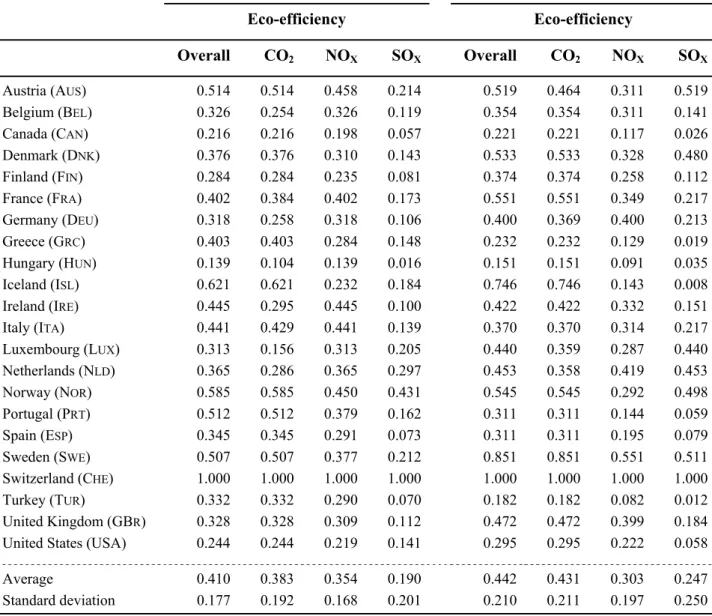
(16) for all. 0,1 and b1. b2 and we finally arrive at a log t regression model of the form of equation. (15) above.. 3. Results and discussion 3.1. Some comments on eco-efficiency. Table 1 displays several descriptive statistics for both overall and pressure-specific scores of ecoefficiency in the years 1980 and 2008. First of all, the average of the eco-efficiency indicators shows an upward trend over the sample period in all the definitions, except for NOX emissions; furthermore, the highest average eco-efficiency scores at specific air pollutant level correspond to CO2 emissions. This seems quite reasonable if we bear in mind that this pollutant is the main contributor to global warming and that environmental regulations aimed at reducing carbon dioxide emissions have been in force the longest and in most cases are the most restrictive.11 Secondly, Switzerland is the only economy that remains on the eco-efficient frontier throughout the entire period studied. In other words, Switzerland is always the most eco-efficient country in the sample. Where overall eco-efficiency is concerned, the second best performing country in 2008 was Sweden, followed by Iceland, France, Norway and Denmark, that is, mostly Scandinavian countries. Conversely, Southern European economies such as Portugal, Spain and Greece, in addition to Hungary, Turkey, Canada and the United States, record the worst eco-efficiency scores. It is also interesting to highlight that overall eco-efficiency in countries such as Portugal, Spain, Greece and Turkey is lower in 1980 than in 2008.12 In contrast, the largest improvements correspond to Sweden, Denmark, France, United Kingdom, Luxembourg and Iceland. Finally, it is worth highlighting. 11. Our scores of overall eco-efficiency are in fact largely determined by eco-efficiency in CO2 emissions, as the. proportional reduction in all three emissions is constrained in most countries by these emissions. In more technical words, due to greater effort being made to reduce CO2 emissions, restrictions on this pollutant in program (3) have more binding power. 12. Kortelainen (2008) obtains the same result for Spain and Greece as regards the evolution of environmental per-. formance between 1990 and 2003.. 14.

(17) the very low economic and ecological performance in NOX emissions of Turkey, Hungary and Canada. The abovementioned results suggest the existence of a relationship between eco-efficiency and economic development. In order to shed some light on this association, we have computed the Spearman correlation coefficient between GDP per capita and our four indicators of eco-efficiency. In 2008, correlations are 0.652, 0.611, 0.419 and 0.475 for overall eco-efficiency and eco-efficiency in CO2, NOX and SOX emissions, respectively. In addition, with the exception of NOX emissions, the relationships are statistically significant at standard confidence levels. However, eco-efficient behaviour cannot be mechanically attributed to richer countries; for example, Luxembourg is by far the richest economy in our sample, but is ranked 10th in terms of overall eco-efficiency. In addition, and in order to make a proper interpretation of our results, it should be noticed that ecoefficiency is heavily conditioned by features such as the sectoral patterns of production or trade and flows of foreign direct investment. In this sense, some economies may decide not to produce contaminating goods in-house but import these goods from more polluting countries, or simply externalise their production to countries with less restrictive environmental regulations while retaining the ownership of the production. Nonetheless, an in-depth analysis of the factors behind differences in eco-efficiency among countries is beyond the scope of this research.. 3.2. Is there eco-efficiency convergence among OECD countries?. In this Section we test for the existence of eco-efficiency convergence clubs using the indicators computed in Section 3.1 and the Phillips and Sul (2007) convergence algorithm described in Section 2.2. The results for overall eco-efficiency emissions as well as for specific eco-efficiency in CO2, NOX and SOX emissions are presented in Table 2 and Graph 1. Concerning overall eco-efficiency, the first column of Table 2 presents the five convergence clubs obtained. We should take into account that the variable of interest is bounded between zero and one, where one denotes the most eco-efficient country, which was Switzerland in all cases. We proceed as follows: we find a first convergence club (Club 1) that consists of Iceland, Sweden and Switzer15.

(18) land. The other nineteen countries do not form a complementary club,13 so we look for a new and smaller convergence club (Club 2) which in this case contains nine countries (Austria, Denmark, France, Germany, Ireland, Luxemburg, the Netherlands, Norway and the United Kingdom). The next club (Club 3) consists of Belgium, Finland, Italy, Portugal, Spain and the United States, whereas Club 4 includes Canada and Greece. Finally, Club 5 has also two members: Hungary and Turkey. We should note that all countries analysed are classified in one of the five convergence clubs. It is also worth mentioning that the speed of convergence is relatively slow for all the emissions considered in Table 2. This information can be gathered from the parameter presented under the heading ‘log t’. This parameter is which is twice the value of , the speed of convergence towards the average, and value of. 0 in the case of convergence. The first group, the best performers, records a. = 0.001. Convergence is faster among other groups, implying that they are approaching. one another more rapidly in relative terms. We should bear in mind that the absolute best performer, Switzerland, is included in the first group. The same information contained in Table 2 can be represented graphically using the relative transition paths, that is, the series of hit for all the countries analysed.14 This relative transition is calculated in relation to the average. Therefore, both the best and worst performing countries will be above and below 1, respectively. Converging implies coming closer to the average, although those countries that are improving should approach Switzerland or, at least, the first convergence club detected. Moreover, countries that are part of a convergence club may behave differently depending on their trajectories (see Phillips and Sul, 2009). We can observe the average relative transition paths of overall eco-efficiency in Graph 1a. The results previously discussed in Table 2 are equally visible in the picture: the three best performers are. 13. The statistic was -28.527 (log t equal to -0.862), so we reject convergence for the group of countries.. 14. Although our discussion will focus on the average relative transition paths of the clubs found, the Appendix. includes the Graphs containing all the countries and pollutants analysed.. 16.

(19) Iceland, Switzerland and Sweden and these are the members of the first convergence club. Concerning their relative transition path, it tends towards a value of 2, clearly below the average and improving. Concerning the second cluster of countries (including a total of nine countries), although their relative transition starts at similar levels to the third group, they are placed above the average and display slow but steady improvement. The third group, in contrast, is below the average and registers a tendency to worsen. The last two groups of countries (Canada, Greece, Hungary and Turkey) are not only the worst performers, but also display a downward trend. Finally, in order to analyse whether it is possible to merge some of the convergence clubs found above, we have followed the method proposed by Phillips and Sul (2009). The results for overall eco-efficiency are presented in Table 3. We reject the null hypothesis of club-merging for all the combinations of two or three clubs. Concerning CO2 emissions, the four convergence clubs found are presented in the second column of Table 2. The first club consists of the same countries found for overall emissions (Iceland, Switzerland and Sweden). In Graph 1b, we can observe that the first club appears distinctively above the average approaching 2. A second convergence club includes eight countries (Austria, Denmark, France, Germany, Ireland, Luxemburg, Norway and the United Kingdom). All the countries in this club display relative convergence towards 1 and their trend is positive and above the average (see Graph 1b). The third club consists of Belgium, Finland, Italy, the Netherlands, Portugal, Spain and the United States. In contrast to the previous group, their trend is negative, so they are dropping further below the average. Finally, Canada, Greece, Hungary and Turkey are the worst performers, but they form a group. Their convergence path diverges toward 0.5. As for the speed of convergence, the picture is similar to that for overall eco-efficiency. Slow convergence is found among the members of Clubs 1 and 3, whereas the members of Clubs 2 and 4 are approaching more rapidly. In addition, we test for club merging and also obtain the same negative results in this case. Table 4 shows the details. Regarding NOX emission eco-efficiency, a similar pattern emerges. The first club consists of Sweden and Switzerland. This club average, shown in Graph 1c, clearly has an upward trend, approach17.

(20) ing 3 and improving relative to the general average. The second convergence club includes Austria, France, Germany, the Netherlands and the United Kingdom. They follow a similar relative transition pattern, although they attain much lower levels. In any case, this group is clearly above the average and has a positive trend. The behaviour is very similar in the case of the next club, which consists of Belgium, Denmark, Finland, Ireland, Italy, Luxemburg, Norway and the United States. Their transition path reaches level 1 at the end of the sample, although convergence evolves at a lower rate. Finally, the fourth club is relatively large and includes the remaining countries. Even though we have found a club, the trend of their transition path is clearly negative and attains such low levels that we may consider them almost a diverging group. In Table 5 we present the clubmerging results for NOX emissions. Inter-group convergence is again rejected for all the combinations analysed. As for the speed of convergence, the fastest is found in Club 2 (0.22) and the slowest again in Club 1 (0.04). Finally, in the case of SOX emissions, we have found just one convergence club, which includes the majority of the countries. The only exceptions are Iceland, Greece and Portugal. However, although the algorithm has detected a convergence club, we should be cautious: log t is negative (-0.366) and the t-statistic is -5.76, so convergence should be rejected. Looking closely at the output obtained, the core group is very large: Switzerland, the Netherlands, Sweden, Germany, France, Italy, the United States, Finland, Belgium, Ireland, the United Kingdom, Spain, Canada, Hungary and Turkey (in strict order). The test statistic for the core group indicates the existence of a club, with log t = 2.935 (t-statistic 8.24). Once the next four members are added (Austria, Denmark, Luxembourg and Norway), the existence of a club is rejected. The most plausible reason would be that the possible club members end up at a higher level (see for example Austria in Graph A4 or Denmark) than the original ones, so in practice there is divergence. Therefore, there are two different patterns: first, the majority of the countries start at similar levels (around 1) with the exception of Switzerland, Norway and the Netherlands, which start at higher levels. However, at the end of the period, some countries improve (Luxembourg, Denmark, Sweden and Austria) and join them at around 2. Second, the rest of the countries do not improve their performance, but actually record slightly worse. 18.

(21) performance (excluding possibly Germany, which reaches 1). This explains why the results from the application of the algorithm, without further consideration, are unclear. A closer look at the results for SOX emissions confirms the discussion above. We separate the core group from the four countries added to form Club 1 in the Phillips and Sul (2007) algorithm. The core group consists of Belgium, Canada, Finland, France, Germany, Hungary, Ireland, Italy, the Netherlands, Spain, Sweden, Switzerland, Turkey, the United Kingdom and the United States. Then we start adding a country at a time and find that it was Denmark that was not part of the club. Therefore, we excluded Denmark from the analysis and applied the procedure to 21 instead of 22 countries this time. The results are presented under the heading ‘excluding DNK’. This time we find three convergence clubs: Club 1 includes Austria, Germany, Luxembourg, the Netherlands, Norway, Sweden and Switzerland, that is, the best performing countries. The second club (Club 2) consists of Finland, France, Ireland, Italy and the United Kingdom. Finally, the third club (Club 3) consists of Canada, Hungary, Portugal and the Unites States. The diverging countries are Belgium, Greece, Iceland, Spain, Turkey and Denmark. The analysis of the relative transition path clearly shows the enormous difference that exists between the best performing countries and the rest. However, although Clubs 2 and 3 are both below the average represented by a value of 1, while Club 2 is approaching this level from the mid-nineties onwards, the worst countries follow a downward sloping trajectory. This is confirmed by the tests for club-merging: the hypothesis is accepted for the case of Clubs 1 and 2 (see Table 6). These clubs exhibit the lowest values for speed of convergence. The merger between Clubs 1 and 2 results in even slower convergence, whereas for Club 3,. =. 0.0065.. 4. Summary and concluding remarks. The simplicity of the concept of economic and ecological efficiency and its inbuilt advantage of considering economics and ecology jointly has received increasing attention in political, academic and business circles. In addition, the assessment of eco-efficiency can be considered a new instrument to provide policymakers with sound information to support decisions that contribute to longer-. 19.

(22) term sustainable development. Accordingly, a burgeoning literature has emerged in the last fifteen years aimed at assessing eco-efficiency at firm, industry or economy-wide level. Starting from the most common definition of eco-efficiency as a relationship between economic performance and ecological performance, our aim is to study the existence of convergence in ecoefficiency among developed economies. For this purpose, we use a sample of 22 OECD countries with data for the period 1980-2008. Concerning the methodology, in a first stage we apply the recent approach to eco-efficiency measurement by Picazo-Tadeo et al. (2011) to compute scores of overall eco-efficiency as well as eco-efficiency in the emission of three specific air pollutants, namely, carbon dioxide, nitrogen oxides and sulphur oxides. In a second stage, we follow Phillips and Sul (2007) to test for the existence of convergence clubs in eco-efficiency. To the best of our knowledge, the study of convergence in eco-efficiency at specific environmental pressure and macro level constitutes our main contribution to previous literature in this field. Our main findings are summarised as follows. First, we find an upward trend in all our ecoefficiency indicators, with the only exception of nitrogen oxide emissions. Greater eco-efficiency corresponds to carbon dioxide emissions, probably due to the more demanding regulations in developed economies regarding this air pollutant. Switzerland is always the best performing country, while other economies that perform well are Sweden, Iceland, Norway and Denmark. In contrast, the worst-performing economies are mostly Southern European countries such as Portugal, Spain and Greece, in addition to Hungary, Turkey, Canada and the United States. A positive and statistically significant relationship between income per capita and economic-ecological performance is also found. In addition, eco-efficiency is greatly influenced by features such as the composition of a country’s economic activity and flows of international trade and direct foreign investment. However, an analysis of these aspects is beyond the scope of this paper. Concerning the analysis of convergence, we find that the most eco-efficient countries tend to form convergence clubs by themselves, whereas the worst performers also tend to form clubs of convergence. Where overall eco-efficiency is concerned, five convergence clubs are found. While Iceland, Sweden and Switzerland form the first club of best performers, Hungary and Turkey form the fifth. 20.

(23) and last convergence club. Similar patterns are found for eco-efficiency in carbon dioxide and nitrogen oxide emissions, whereas in the case of sulphur emissions we find three convergence clubs including the majority of the countries in the sample. The main policy implication of our results is that more stringent regulations on air polluting emissions are required in developed economies, particularly in countries displaying lower eco-efficiency levels. Furthermore, while the environmental regulations and intergovernmental agreements put into practice to date have mainly focused on carbon dioxide emissions, future regulations and accords should pay close attention to reducing nitrogen and sulphur oxide emissions, for which developed countries record lower eco-efficiency scores. Finally, we would like to highlight that our research analyses convergence in eco-efficiency at country and environmental pressure level, but further work is required in a topic of such interest to society and with great potential to help policymakers to design better environmental policies. In this sense, incorporating appropriate sectoral disaggregation of economic activity in the assessment of eco-efficiency or relating eco-efficiency scores to foreign direct investment flows, particularly those related to the vertical integration of production processes, are interesting avenues for further research. Accounting for more comprehensive and precise measures of pollution, the construction of composite indicators of environmental pressures with non-linear structures, including some weight restrictions in line with recent work by Zhou et al. (2010), developing more powerful methods to assess convergence or investigating into the determinants of eco-efficiency convergence are also interesting topics for future work. Broadening our knowledge in these directions is undoubtedly one of the greatest challenges for future research in relation to sustainability.. References. Aldy JE (2007) Divergence in state-level per capita carbon dioxide emissions. Land Econ 83:353– 369 Aldy JE (2006) Per capita carbon dioxide emissions: Convergence or divergence? Environ Resour Econ 33:533–555 21.

(24) Allen R, Thanassoulis E (2004) Improving envelopment in data envelopment analysis. Eur J Oper Res 154:363–379 Barassi MR, Cole MA, Elliott RJR (2008) Stochastic divergence or convergence of per capita carbon dioxide emissions: Re-examining the evidence. Environ Resour Econ 40:121–137 Barassi MR, Cole MA, Elliott, RJR (2011) The stochastic convergence of CO2 emissions: A long memory approach. Environ Resour Econ 49:367–385 Camarero M, Picazo-Tadeo AJ, Tamarit C (2008) Is the environmental performance of industrialized countries converging? A ‘SURE’ approach to testing for convergence. Ecol Econ 66; 653– 661 Camarero M, Picazo-Tadeo AJ, Tamarit C (2012) Are the determinants of CO2 emissions converging among OECD countries? Econ Lett, doi:10.1016/j.econlet.2012.10.009. Charnes A, Cooper WW, Rhodes E (1978) Measuring the efficiency of decision making units. Eur J Oper Res 2: 429–444 Cooper WW, Seiford LM, Tone K (2007) Data Envelopment Analysis. A comprehensive text with models, applications, references and DEA-Solver software. Springer, New York Ezcurra R (2007) Is there cross-country convergence in carbon dioxide emissions? Energ Policy 35:1363–1372 Farrell MJ (1957) The measurement of productive efficiency. J Roy Stat Soc A Sta 120: 253-281 Figge F, Hahn T (2004) Sustainable value added–measuring corporate contributions to sustainability beyond eco-efficiency. Ecol Econ 48:173–187 Huppes G, Ishikawa M (2005) A framework for quantified eco-efficiency analysis. J Ind Ecol 9:25– 41 IPCC, Intergovernmental Panel on Climate Change (1990) Climate change: The IPCC scientific assessment. In: Houghton JT, Jenkins GJ, Ephraums JJ (eds.) The IPCC scientific assessment. Cambridge University Press, Cambridge. 22.

(25) IPCC, Intergovernmental Panel on Climate Change (2007) Climate change 2007: Synthesis report. Geneva, Switzerland Jobert T, Karanfil F, Tykhonenko A (2010) Convergence of per capita carbon dioxide emissions in the EU: Legend or reality? Energ Econ 32:1364–1373 Koopmans T (1951) Analysis of production as an efficient combination of activities. In: Koopmans T (ed.) Activity analysis of production and allocation. John Wiley & Sons, New York Kortelainen M (2008) Dynamic environmental performance analysis: A Malmquist index approach. Ecol Econ 64:701-715 Kuosmanen T, Kortelainen M (2005) Measuring eco-efficiency of production with Data Envelopment Analysis. J Ind Ecol 9, 59-72 Lanne M, Liski M (2004) Trends and breaks in per-capita carbon dioxide emissions, 1870–2028. Energy J 25:41–65 Lee C, Chang C (2008) New evidence on the convergence of per capita carbon dioxide emissions from panel seemingly unrelated regressions augmented Dickey-Fuller tests. Energy 33:1468– 1475 Lee C, Chang C (2009) Stochastic convergence of per capita carbon dioxide emissions and multiple structural breaks in OECD countries. Econ Model 26:1375–1381 Nourry M (2009) Re-examining the empirical evidence for stochastic convergence of two air pollutants with a pair-wise approach. Environ Resour Econ 44:555–570 Organization for Economic Cooperation and Development, OECD (1998) Eco-efficiency, OECD, Paris Ordás Criado C, Grether JM (2011) Convergence in per capita CO2 emissions: A robust distributional approach. Resour Energy Econ 33:637–665 Panopoulou E, Pantelidis T (2009) Club convergence in carbon dioxide emissions. Environ Resour Econ 44:47–70. 23.

(26) Phillips PCB, Sul D (2007) Transition modeling and econometric convergence tests. Econometrica 75:1771–1855 Phillips PCB, Sul D (2009) Economic transition and growth. J Appl Econom 24, 1153–1185 Picazo-Tadeo AJ, Reig-Martínez E, Gómez-Limón JA (2011) Assessing farming eco-efficiency: a Data Envelopment Analysis approach. J Environ Manage 92:1154–1164 Porter ME, van der Linde C (1995) Toward a new conception of the environment–competitiveness relationship. J Econ Perspect 9:97–118 Romero-Ávila D (2008) Convergence in carbon dioxide emissions among industrialized countries revisited. Energ Econ 30:2265–2282 Schaltegger S (1996) Corporate environmental accounting. John Wiley and Sons Ltd, Chichester Schmidheiny S, Zorraquin FJL (1996) Financing change, the financial community, eco-efficiency and sustainable development. MIT Press, Cambridge, MA Torgersen A, Førsund F, Kittelsen S (1996) Slack-adjusted efficiency measures and ranking of efficient units. J Prod Anal 7:379–398 United Nations (2009) Eco-efficiency indicators: Measuring resource-use efficiency and the impact of economic activities on the environment. Greening of Economic Growth Series, ST/ESCAP/2561 WBCSD, World Business Council for Sustainable Development (2000) Eco-efficiency: creating more value with less impact. WBSCD, Geneva. Westerlund J, Basher S (2008) Testing for convergence in carbon dioxide emissions using a century of panel data. Environ Resour Econ 40:109–120 Wursthorn S, Poganietz WR, Schebek L (2011) Economic-environmental monitoring indicators for European countries: A disaggregated sector-based approach for monitoring eco-efficiency. Ecol Econ 70:487–496. 24.

(27) Zhang B, Bi J, Fan Z, Yuan Z, Ge J (2008) Eco-efficiency analysis of industrial system in China: A data envelopment analysis approach. Ecol Econ 68:306–316 Zhou P, Ang BW, Poh KL (2008) A survey of data envelopment analysis in energy and environmental Studies. Eur J Oper Res 189:1–18 Zhou P, Ang BW, Zhou DQ (2010) Weighting and aggregation in composite indicator construction: a multiplicative optimization approach. Soc Indic Res 96:169–181. 25.

(28) Table 1. Scores of overall and pressure-specific eco-efficiency Year 1980. Year 2008. Eco-efficiency. Eco-efficiency. Overall. CO2. NOX. SOX. Overall. CO2. NOX. SOX. Austria (AUS) Belgium (BEL) Canada (CAN) Denmark (DNK) Finland (FIN) France (FRA) Germany (DEU) Greece (GRC) Hungary (HUN) Iceland (ISL) Ireland (IRE) Italy (ITA) Luxembourg (LUX) Netherlands (NLD) Norway (NOR) Portugal (PRT) Spain (ESP) Sweden (SWE) Switzerland (CHE) Turkey (TUR) United Kingdom (GBR) United States (USA). 0.514 0.326 0.216 0.376 0.284 0.402 0.318 0.403 0.139 0.621 0.445 0.441 0.313 0.365 0.585 0.512 0.345 0.507 1.000 0.332 0.328 0.244. 0.514 0.254 0.216 0.376 0.284 0.384 0.258 0.403 0.104 0.621 0.295 0.429 0.156 0.286 0.585 0.512 0.345 0.507 1.000 0.332 0.328 0.244. 0.458 0.326 0.198 0.310 0.235 0.402 0.318 0.284 0.139 0.232 0.445 0.441 0.313 0.365 0.450 0.379 0.291 0.377 1.000 0.290 0.309 0.219. 0.214 0.119 0.057 0.143 0.081 0.173 0.106 0.148 0.016 0.184 0.100 0.139 0.205 0.297 0.431 0.162 0.073 0.212 1.000 0.070 0.112 0.141. 0.519 0.354 0.221 0.533 0.374 0.551 0.400 0.232 0.151 0.746 0.422 0.370 0.440 0.453 0.545 0.311 0.311 0.851 1.000 0.182 0.472 0.295. 0.464 0.354 0.221 0.533 0.374 0.551 0.369 0.232 0.151 0.746 0.422 0.370 0.359 0.358 0.545 0.311 0.311 0.851 1.000 0.182 0.472 0.295. 0.311 0.311 0.117 0.328 0.258 0.349 0.400 0.129 0.091 0.143 0.332 0.314 0.287 0.419 0.292 0.144 0.195 0.551 1.000 0.082 0.399 0.222. 0.519 0.141 0.026 0.480 0.112 0.217 0.213 0.019 0.035 0.008 0.151 0.217 0.440 0.453 0.498 0.059 0.079 0.511 1.000 0.012 0.184 0.058. Average Standard deviation. 0.410 0.177. 0.383 0.192. 0.354 0.168. 0.190 0.201. 0.442 0.210. 0.431 0.211. 0.303 0.197. 0.247 0.250. 26.

(29) Table 2. Convergence club classification. Overall eco-efficiency. Eco-efficiency in CO2 emissions. Eco-efficiency in NOX emissions. Eco-efficiency in SOX emissions. Club 1 [ISL, CHE, SWE]. Club 1 [ISL, CHE, SWE]. Club 1 [CHE, SWE]. Divergence. log t 0.002. t-stat 0.030. Club 2 [AUS, DNK, FRA, DEU, IRE, LUX, NLD, NOR, GBR] log t 0.012. t-stat 0.108. Club 3 [BEL, FIN, ITA, PRT, ESP, USA] log t 0.166. t-stat 9.048. Club 4 [CAN, GRC] log t 0.404. t-stat 12.04. log t 0.002. t-stat 0.030. log t 0.079. Club 2 [AUS, DNK, FRA, DEU, IRE, LUX, NOR, GBR] log t 0.254. t-stat 2.603. log t 0.121. t-stat 2.526. t-stat 1.126. Club 4 [CAN, ISL, ESP, PRT, GRC, TUR, HUN]. t-stat 5.744. log t 0.331. Club 5 [HUN, TUR] log t 0.471. t-stat 2.174. Club 3 [BEL, DNK, FIN, IRE, ITA, LUX, NOR, USA] log t 0.081. Club 4 [CAN, GRC, HUN, TUR] log t 0.315. Club 2 [AUS, FRA, DEU, NLD, GBR] log t 0.440. Club 3 [BEL, FIN, ITA, NLD, PRT, ESP, USA]. t-stat 1.313. t-stat 1.162. log t -0.366. t-stat -5.76**. Club 1 (excluding DNK) [AUS, DEU, LUX, NLD, NOR, CHE, SWE,] log t 0.173. t -stat 1.751. Club 2 (excluding DNK) [FIN, FRA, IRE, ITA, GBR] log t 0.087. t-stat 0.544. Club 3 (Excluding DNK) [CAN, HUN, PRT, USA] log t 0.219. t-stat 2.79. Non converging [BEL, GRC, ISL, ESP, TUR, DNK]. t-stat 3.84. log t -2.285. t-stat -29.526**. Note: The clubs reported in this table have been obtained from the application of the algorithm proposed by Phillips and Sul (2007). ‘log t’ stands for the parameter ˆ in equation (15), which is twice the speed of convergence, denoted as , of this club towards the average; ‘t-stat’ is the convergence test statistic, distributed as a simple one-sided t-test (i.e. the critical value is -1.65).. 27.

(30) Table 3. Convergence club classification: Overall eco-efficiency Initial classification (t of ) Club 1 [3]. 0.002 (0.030). Club 2 [9]. 0.012 (0.108). Club 3 [6]. 0.166 (9.048). Club 4 [2]. 0.404 (12.04). Tests of club merging (t of ). Final classification (t of ). Club 1+2 -0.363 (-7.88)** Club 2+3 -0.576 (-7.58)** Club 2+3+4 -0.678 (-12.15)** Club 3+4 -0.346. Club 1 [3]. 0.002 (0.030). Club 2 [9]. 0.012 (0.108). Club 3 [6]. 0.166 (9.048). Club 4 [2]. 0.404 (12.04). Club 5 [2]. 0.471. (-56.36)** Club 5 [2]. 0.471 (3.84). (3.84). Note: The left-hand-side column includes the initial club classification, where the number of countries in each club appears in brackets. The tests of club merging have as a null hypothesis that Club i and Club j can be considered a joint convergence club. The test is also distributed as a one-sided t-statistic with a 5% critical value of -1.65. Two asterisks denote rejection. The right-hand-side column includes the final club classification.. Table 4. Convergence club classification: eco-efficiency in CO2 emissions Initial classification (t of ) Club 1 [3]. 0.002 (0.030). Club 2 [8]. 0.254 (2.603). Club 3 [7]. 0.121 (2.526). Club 4 [4]. 0.315 (5.744). Tests of club merging (t of ) Club 1+2 -0.21 (-14.13)** Club 2+3 -0.369 (-7.157)** Club 2+3+4 -0.507 (-11.78)**. Final classification (t of ) Club 1 [3]. 0.002 (0.030). Club 2 [8]. 0.254 (2.603). Club 3 [7]. 0.121 (2.526). Club 4 [4]. -0.315 (5.744). Note: The left-hand-side column includes the initial club classification, where the number of countries in each club appears in brackets. The tests of club merging have as a null hypothesis that Club i and Club j can be considered a joint convergence club. The test is also distributed as a one-sided t statistic with a 5% critical value of -1.65. Two asterisks denote rejection. The right-hand-side column includes the final club classification.. 28.

(31) Table 5. Convergence club classification: eco-efficiency in NOX emissions Initial classification (t of ) Club 1 [2]. 0.079 (1.313). Club 2 [5]. 0.404 (2.174). Club 3 [8]. Club 4 [7]. Tests of club merging (t of ). Final classification (t of ) Club 1 [2]. 0.079 (1.313). Club 2 [5]. 0.404 (2.174). 0.081 (1.126). Club 3 [8]. 0.081 (1.126). 0.331 (1.162). Club 4 [7]. 0.331 (1.162). Club 1+2 -5.109 (-10.495)** Club 2+3 -0.338 (-6.291)**. Note: The left-hand-side column includes the initial club classification, where the number of countries in each club appears in brackets. The tests of club merging have as a null hypothesis that Club i and Club j can be considered a joint convergence club. The test is also distributed as a one-sided t statistic with a 5% critical value of -1.65. Two asterisks denote rejection. The right-hand-side column includes the final club classification.. Table 6. Convergence club classification: eco-efficiency in SOX emissions Initial classification (t of ) Club 1 [7]. 0.173 (1.751). Club 2 [5]. 0.087 (0.544). Club 3 [4]. Nonconvergence [6]. Tests of club merging (t of ). Final classification (t of ) Club 1+2 [12]. 0.013 (0.181). 0.219 (2.79). Club 3 [4]. 0.219 (2.79). -2.285 (-29.526)**. Nonconvergence [6]. -2.285 (-29.526)**. Club 1+2 0.013 (0.181) Club 2+3 -0.935 (-20.735)**. Note: The left-hand-side column includes the initial club classification, where the number of countries in each club appears in brackets. The tests of club merging have as a null hypothesis that Club i and Club j can be considered a joint convergence club. The test is also distributed as a one-sided t-statistic with a 5% critical value of -1.65. Two asterisks denote rejection. The right-hand-side column includes the final club classification.. 29.

(32) Graph 1. Relative transition paths. Averages for the convergence clubs obtained in the Phillips and Sul (2007) analysis. Graph 1a. Overall eco-efficiency.. Graph 1b. Eco-efficiency in CO2 emissions.. 30.

(33) Graph 1. Relative transition paths. Averages for the convergence clubs obtained in the Phillips and Sul (2007) analysis (continued). Graph 1c. Eco-efficiency in NOx emissions.. Graph 1d. Eco-efficiency in SOx emissions.. 31.

(34)