SOCIO−ECONOMIC STATUS AND HEALTH: EVIDENCE FROM THE ECHP

SOCIO−ECONOMIC STATUS AND HEALTH:

EVIDENCE FROM THE ECHP

David Cantarero Marta Pascual

Department of Economics. University of Cantabria Department of Economics. University of Cantabria

Abstract

In this paper, the effects of socioeconomic characteristics (gender, age, education level, marital status, income, occupational and health status, household size and social

relationships) on individuals´ health status in Spain from 1994 to 2001 are analysed. The estimations are carried out using ordered probit models and new data from the whole waves of the European Community Household Panel (ECHP) have been used. The results indicate that personal characteristics, education level, income as well as health status and social relationships have strong influence on self−assessed health.

The authors would like to acknowledge the help given by the Centre for Health Economics (CHE) of the University of York (United Kingdom). Also, we are very grateful for many helpful comments from the participants in the York Seminars in Health Econometrics (YSHE).

1. INTRODUCTION

Since the last years, policy makers have shown an increased interest on population health and, in particular, on those characteristics of individuals that are related to health. Thus, the study of population health is an important goal in modern societies and demands careful attention for economic analysis.

However, health is conceptually a complex matter and therefore difficult to measure. Also, there have not existed until recent years reliable data which measure individuals´ health status. By this way, individuals’ health has being specified as an individual characteristic function based on different inputs (Grossman, 1972; Bound, 1990; Smith, 1999; Fuchs, 2004). In this sense, one of the most commonly used indicators of individuals’ health status is Self-Assessed Health (SAH) which is based on a very simple question: “how is your health in general?”, with response categories ranging from “very good” or “excellent” to “bad” or “very bad". The problem with the arrival of survey data which include this kind of health measures is that information about individuals’ health is only available in an ordinal way (Van Doorslaer and Jones, 2003).

Although this SAH variable is usually supplemented by a host of other measurement instruments, its use remains very popular in general socioeconomic surveys. By this way, SAH has been used in previous studies of the relationship between health and socioeconomic status (Benzeval et al., 2000; Salas, 2002; Adams et al., 2003; Fritjers et al., 2003) and between health and lifestyles (Contoyannis and Jones, 2004). Also, it has been demonstrated that SAH can be a good predictor of use of medical care (Van Doorslaer et al., 2002) and mortality inequalities (Van Doorslaer and Gerdtham, 2003).

However, the validity of this subjective measure of health (SAH) has being discussed widely in health economics literature. Thus, SAH might be prone to measurement error (Van Doorslaer and Jones, 2003; Crossley and Kennedy, 2002). Furthermore, reporting bias and heterogeneity in the measure of SAH can be detected (Hernández-Quevedo et al., 2004). In some cases, the “true health” map into SAH categories may vary with individuals´ characteristics who respond in the survey. This type of measurement error occurs if subgroups of the population use different cut-point levels when reporting their SAH, despite having the same level of “true health” (Groot, 2000). In fact, there exists a growing literature which evaluate bias in SAH data being significant the systematic use of different thresholds for populations subgroups (Lindeboom and Van Doorslaer, 2003; Van Doorslaer and Jones, 2003). These differences can be influenced, among other factors, by age, gender, education, income and previous illnesses. In summary, it supposes that different groups interpret the question about their SAH in their own personal framework and they use different reference points when respond to the same question.

The problem of an ordinal scale can be solved creating a dichotomy variable for healthy or not healthy status or arbitrarily by the imposition of some type of order. However, the use of a dichotomy variable has several disadvantages since not the whole variation of health that is caught in the variable related to SAH is used and makes the comparisons of inequality over the time or among population segments not very reliable. By this way, the results would depend on the election of the threshold that consider healthy people versus non-healthy people (Lindeboom

and Van Doorslaer, 2003). Another alternative consists on assumming that the underlying category of the empiric distribution of the answers related to the SAH is a latent variable. This last approach will be adopted in this study.

The objective of this paper is to analyze the effect of diverse socioeconomic characteristics (gender, age, education, marital status, income, occupational and health status and social relationships) on individuals´ health status in Spain since 1994 to 2001. New data from the European Community Household Panel (ECHP) have been used. This source of information contains homogeneous data among the European Union countries and it is harmonized at European level. The ECHP includes a measure of SAH in the sense that, among the available health variables, it reports individuals’ health status and orders them in a scale of five categories or attributes.

The structure of the paper is as follows. The ECHP data set and the self-assessed health variable are described in Section 2. Section 3 is focused on the relationship between health, income and other socio-economic variables in Spain using ordered probit models. Finally, conclusions are presented in Section 4.

2. DATA AND METHODOLOGICAL DECISIONS: THE EUROPEAN COMMUNITY HOUSEHOLD PANEL (ECHP)

The ECHP is a representative database of households of different European Union countries, it was elaborated for the first time in 1994 and it was composed by 60.500 households (approximately 170.000 individuals). In the case of Spain, the first wave was composed by 7.206 households (23.025 individuals). TABLE I includes information about households and individuals´ sample composition for Spain.

This new survey contains data on individuals and households for the European Union countries with eight waves available (1994-2001). The main advantage is that information is homogeneous among countries since the questionnaire is similar across them. This source of data is coordinated by the European Commission's Statistical Office (EUROSTAT). Also, this survey includes rich new information about income, education, employment, health, etc. In this sense, it is important to highlight that it is the first fixed and harmonized panel for studying socio-economic factors of the households and individuals inside the European Union.

The variable we use as a proxy of individual’s health status is the SAH that each individual reports of their own health status and the possible responses are ordered qualitatively. Thus, SAH variable is a subjective response to the question “How is your health in general?” and it takes the values “1” (very good), “2” (good), “3” (fair), “4” (bad) and “5” (very bad). This variable is also included in other longitudinal surveys, such as the British Household Panel Survey (BHPS) in the case of the United Kingdom, the Canadian National Population Health Survey (NPHS) for Canada, the National Health Interview Survey (NHIS) for United States, etc., and it has facilitated recent research on individuals’ health status explanation. However, there are large differences in SAH status between the European Union countries (see TABLE II). For

example, in 2001, Ireland, Greece and Denmark reported the best health status while Portugal, Germany, France, Italy and Spain reported the worst one. However, the differences between countries are not completely convincing as judged by other health measures, such as life expectancy.

Thus, according to World Health Organization (2000), life expectancy at birth is longest in France, Italy and Spain and shortest in Ireland and Denmark. TABLE III shows relative frecuencies for the classifications of SAH in Spain and we can observe a clear improvement in the frequency of reporting “good” health since 1994 to 2001 and approximately half of people interviewed report that their SAH is “good”.

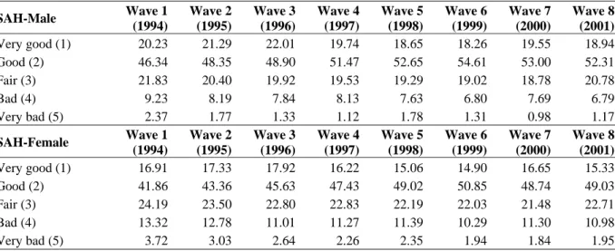
However, it is important to point out the different distribution of SAH by gender (TABLE IV). In this sense, men report better levels of SAH than women. This fact might reflect the different perception of health by gender (maybe because men´s life expectancy is shorter than women´s). Another possible explanation of gender differentials, especially at older ages, is the mortality selection (Ahn, 2002). In this case, as the mortality rate is higher for men than for women, those who survive in higher mortality environment are on average genetically stronger than the survivors in lower mortality environment.

Finally, FIGURE 1 shows the distribution of SAH for each wave, using the Spanish balanced panel of individuals who are observed for the whole 8 waves. The different categories are shown on the horizontal axis with “1” representing the highest level of health and “5” the lowest. The histograms have a similar pattern and we can observe a skewed distribution with the majority of individuals reporting that their health is good.

3. SOCIO-ECONOMIC STATUS AND SELF-ASSESSED HEALTH INEQUALITIES IN SPAIN: AN EMPIRICAL APPROACH BASED ON

ORDERED PROBIT MODELS

In the last years new techniques allow us to deepen in the study of multinomial choice variables (Greene, 2003; Jones, 2000). In particular, we will focus our analysis on individuals´ SAH. This variable takes five values that vary from “very bad” to “very good”. The logit multinomial and probit multinomial models do not take into account that dependent variable reflects an order. In this way, regression analysis of SAH can be achieved through specifying an ordered probit model. Thus, our starting model is formulated through a latent health variable H* that it is unobserved (an individual's “true” health) and which depends on a lineal combination of explanatory variables:

ε

β′ +

= x

H* , (1)

where x is a set of explanatory variables, β a set of coefficients and ε an error term uncorrelated with the set of regressors with a normal distribution.

The dependent variable used is individual report of SAH. Thus, the higher value of our latent variable, the higher will be the probability that the individual reports a higher category in the self-assessed health scale.

However, H* is unobserved and what we do observe is: ⎪ ⎪ ⎩ ⎪ ⎪ ⎨ ⎧ ≥ − ≥ ≥ ≥ = − )1 ( * 1 1 * 1 2 * 1 1 ) 1 ( ... ... ... 1 0 M i H if M H if H if H γ γ γ γ (2)

where γ₁,γ₂,...,γ_(M−1) are unknown parameters to be estimated with β . The probabilities of each category are: ) ( 1 ) , , / ) 1 ( Pr( ... ) ( ) ( ) , , / 1 Pr( ) ( ) , , / 0 Pr( ) 1 ( 1 2 1 β γ γ β β γ β γ γ β β γ γ β i M i i i i i i i i i X X M H X X X H X X H − Φ − = − = − Φ − − Φ = = − Φ = = − (3)

where function Φ denotes the standard normal distribution. (.)

The corresponding estimators are obtained maximizing the log-likelihood function:

[

]

_∑

[

]

_∑

[

]

∑

− = = = − = + + = + = = Γ ) 1 ( 1 0 ) , , / ) 1 ( Pr( log ... ) , , / 1 Pr( log ) , , / 0 Pr( log ) , ( M Y i i Y i i Y i i X H X H M X H

β

γ

β

γ

β

γ

γ

β

_{. (4)}

The sign of the coefficients shows the tendency of the variation in the probability of belonging to the highest answer due to an increment in the corresponding explanatory variable and the marginal effect of a regressor on the probability of belonging to each category is as follows:

[

]

k i M k k i i k k i k X X M H X X X H X X H β β γ β β γ β γ β β γ ) ( ) 1 Pr( ... , ) ( ) ( ) 1 Pr( , ) ( ) 0 Pr( ) 1 ( 1 2 1 − Φ − = ∂ − = ∂ − Φ + − Φ − = ∂ = ∂ − Φ − = ∂ = ∂ − (5)

So, marginal effect of a regressor Xk depends on the coefficient value βk and on the

values of a normal density function Φ for each person. (.)

In order to establish the main factors which affect health levels, we have classified them into seven groups of variables: personal characteristics, education level, marital status, income, occupational status and other variables related to individuals’ health, household characteristics and social relationships.

Firstly, as personal characteristics we have included two variables: individual’s age and gender. To allow for a flexible relationship between the SAH and age, a quartic polynomial

AGE4=Age4/1,000,000). Also, the gender of individuals has been taken into consideration and a dummy variable which takes value of 1 if individual is male has been built.

The second group of variables are refered to the maximum level of education completed. In the ECHP, education is classified into three categories based on ISCED classification: less than secondary level (ISCED 0-2), second stage of secondary level (ISCED 3) and third level (ISCED 5-7). Thus, two dummy variables have been included: third level of education (HEDUC) and another one for second stage of secondary level (SSEDUC). In this sense, many studies have shown that education is an important socioeconomic characteristic in determining health status, so the attainment of higher educational levels can be reflecting important changes in SAH.

Thirdly, representing marital status, we have considered four variables (never married, separated, divorced and widow) with married as the reference category.

On the other hand, we are concerned with the influence of income on health status. In fact, higher income should be associated with better health although this relationship is not clear and correlation can vary from highly positive to weakly negative, depending on context, covariates and level of aggregation (Fuchs, 2004). Our income variable is equivalised annual net household income (LINCOMEOCDMO) adjusted using OECD modified scale to take into account household size and composition. In this sense, we have used household information rendering the component family by using equivalence scales. The modified OECD scale gives a weight of 1 to the first adult, 0.5 to other persons aged 14 or over and 0.3 to each child aged less than 14. For each person, the “equivalised total net income” is calculated as its household total net income divided by equivalised household size. In this case, we use the logarithm of household´s income (OECD modified scale) taking into account the concavity in the health-income relationship (Gravelle, 1998; Jones and Wildman, 2004).

Other variables included in the analysis related to occupational status are status in employment and working in the public sector. We have considered a dummy variable that takes the value one if the individual is working with an employer in paid employment as a salaried and zero otherwise (SALA) and another one which takes the value one if current job is in the public sector (including non-profit private organisations) and zero otherwise (PUBLI).

Also, we have considered other variables related to health status. The variable IN-PATIENT indicates whether or not the individual has been admitted to a hospital during the past 12 months. The variable CDACTSM (cut down acts/mental condition) reflects whether or not the individual has had to cut down some activities in home, at work or in their leisure time, due to an emotional or mental health problem.

Finally, we have considered number of people in household including respondents (Household size-HHSIZE). Also, we have included variables related to social relationships, and another dummy variable has been built in order to take into account whether an individual is a member of a club or organisation (SOCIALCL) or not. TABLE V shows explanatory variables used in estimations and their corresponding definitions.

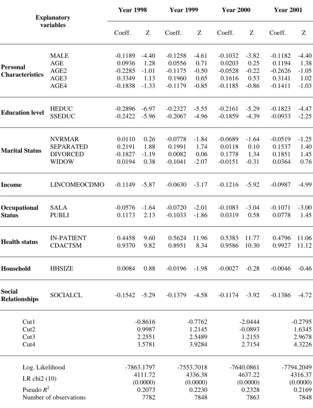
We have used ordered probit models, because they have several advantages compared with other econometric methods in the treatment of categorical ordered variables as in our case. Results have been obtained using STATA 8.0. Estimation of the models are based on the method of maximum likelihood and results for the case of Spain in 1994-2001 are presented in TABLE VI.

A first point to note is that most of coefficients of the explanatory variables are very stable for the eight waves, in particular, those related to personal characteristics, education level, income, health status and social relationships. Because of SAH appears in the ECHP on a scale from “1” to “5”, where “1” corresponds to very good health and “5” to very bad, a negative sign in the coefficients implies an increase in the probability of reporting good health.

Thus, we can observe that some personal characteristics, such as being male, have a positive and significant impact on individuals’ health while individuals’ age has a negative one reflecting the on-going general deterioration of health. The education coefficients maintain statistical significance showing that more education leads to an increase in the probability of reporting good health. Marital status variables (never married, separated, divorced, widow) have not a clear positive or negative sign and it varies among the different waves although have an important impact on individual´s health. Also, we can observe that income coefficient is always significance and has a positive effect on reporting good health. With respect to occupational status variables, salaried and working in public sector have a positive effect on individuals´ health in most of the waves. On the other hand, the two variables related to health status (IN-PATIENT and CDACTSM) increase the probability of individual reporting bad health status as expected. Household size has not a clear positive or negative sign and again it varies among the different waves. Finally, social relationships have a positive effect on health status.

Finally, it is important to note that in the whole years, the models account for about 20% of the variation of the health transition probabilities, based on the values of the pseudo-R squared statistics. TABLE VI also includes estimates of the threshold parameters γ1,γ2,γ3 and γ4 (denoted as Cut1, Cut2, Cut3 and Cut4). These imply that, for example, in 2001, a value of the latent variable less than -0.2795 corresponds to very good health, a value between -0.2795 and 1.6345 corresponds to good health, a value between 1.6345 and 2.9678 corresponds to fair health, a value between 2.9678 and 4.3226 corresponds to bad health and a value above 4.3226 corresponds to very bad health. Thus, the predicted value of H* for the reference individual (where all the explanatory variables equal zero) lies between –0.2795 and 1.6345, hence the reference individual would be predicted to report good health in 2001. So, the cutpoints can be interpreted in terms of z-scores (Greene, 2003). That is, the boundary between very good and good health is at z=−0.2795, the boundary between good and fair health is at 1.6345, the boundary between fair and bad health is at 2.9678 and the boundary between bad and very bad health is at 4.3226. These values leave Φ(−0.28)=0.3897 or 38.97% of the reference group in the very good health category, Φ(1.63)−Φ(−0.28)=0.5587 or 55.87% of the reference group in the good health category, 5.01% in the fair health category and only 0.15% of the reference group in the bad health category.

4. CONCLUSIONS

In this paper, we have developed different ordered probit models in order to identify interactions between health (self-assessed health) and different explanatory factors in Spain from 1994 to 2001. Results from microdata of ECHP indicate, firstly, that income has positive effects on health so an income redistribution to poor population groups could raise average health status and decrease health inequalities given the concativity of the relationship between income and health. This is a very important conclusion that remains constant for the eight years considered.

Nevertheless, the analysis of Spanish individual’s health status suggests that not only income, but also other variables such as gender (male), education level and social relationships have a positive impact on self-assessed health. Other factors such as age and other variables related to health status (hospital admission and cut down acts/mental condition) have a negative effect.

Finally, the results have important implications for health and welfare state policies and provide more empirical evidence about the relationship between health and different socioeconomic factors using individual data in Spain. By this way, as average education level of Spanish population is increasing and better educated younger generations are replacing older ones (with lower levels of education), it is expected a shift on population health status.

REFERENCES

Adams, P., Hurd, M.D., McFadden, D., Merrill, A., Ribeiro, T. (2003) “Healthy, wealthy and wise? Tests for direct causal paths between health and socioeconomic status” Journal of Econometrics, 112, 3-56

Ahn, N. (2002) “Assessing Self-Assessed Health Data” Working Paper 2002-24, FEDEA, Madrid.

Benzeval, M., Taylor, J., Judge, K. (2000) “Evidence on the relationship between low income and poor health: Is the Government doing enough?” Fiscal Studies, 21(3), pp. 375-399. Bound, J. (1990) “Self-Reported versus objective measures of health in retirement models” The

Journal of Human Resources, XXVI.

Contoyannis, P., Jones, A. (2004) “Socio-economic status, health and lifestyle” Journal of Health Economics, 23, 965-995.

Contoyannis, P., Jones, A., Rice, N. (2004) “The dynamics of health in the British Household Panel Survey” Journal of Applied Econometrics, 19 (4), 473-503.

Crossley, T.F., Kennedy, S. (2002) “The reliability of self-assessed health status” Journal of Health Economics, 21, 643-658.

Fritjers, P., Haisken-DeNew, J.P., Shields, M.A. (2003) “Estimating the causal effect of income on health: Evidence from post reunification East Germany” Centre for Economic Policy Discussion Paper, No. 465, Australian National University.

Fuchs, V.R. (2004) “Reflections on the socio-economic correlates of health” Journal of Health Economics, 23, 653-661.

Gravelle, H. (1998) “How much of the relation between population mortality and unequal distribution of income is a statistical artefact?” British Medical Journal, 316, no. 7128, 382-385.

Greene, W.H. (2003) Econometric Analysis, 5th Edition, Prentice Hall: Englewood Cliffs.

Groot, W. (2000) “Adaptation and scale of reference bias in self-assessments of quality of life” Journal of Health Economics, 19 (3), 403-420.

Grossman, M. (1972) “On the concept of health capital and the demand for health” Journal of Political Economy, 80 (2), 223-255.

Hernandez-Quevedo, C., Jones, A.M., Rice, N. (2004) “Reporting bias and heterogeneity in self-assessed health. Evidence from British Household Panel Survey” Ecuity III Project Working Paper, Nº 19.

Jones, A.M. (2000) “Health Econometrics”, In Culyer, A.J. and Newhouse, J.P. (eds.): Handbook of Health Economics, Elsevier, Amsterdan.

Jones, A.M., Wildman, J. (2004) “Disentangling the relationship between health and income” Ecuity III Project Working Paper, Nº 4.

Lindeboom, M., Van Doorslaer, E. (2003) “Cut-point shift and index shift in self reported health” Journal of Health Economics, 23, Issue 6, 1083-1099.

Salas, C. (2002) “On the empirical association between poor health and low socioeconomic status at old age” Health Economics, 11, pp. 207-220.

Smith, J.P. (1999) “Healthy bodies and thick wallets: the dual relationship between health and economic status” Journal of Economic Perspectives, 13, pp. 145-166.

Van Doorslaer, E., Gerdtham, U.G. (2003) “Does inequality in self-assessed health predict inequality in survival by income? Evidence from Swedish data” Social Science and Medicine,

Van Doorslaer, E., Koolman, X., Jones, A. (2002) “Explaining income-related inequalities in doctor utilisation in Europe: a decomposition approach” Ecuity II Project Working Paper, 5. Van Doorslaer, E., Jones, A. (2003) “Inequalities in self-reported health: validation of a new

approach to measurement” Journal of Health Economics, 22, Issue 1, pp. 61-78. World Health Organization (2000) The World Health Report 2000, WHO.

Figures and Tables

Table I

Household´s sample composition in ECHP (1994-2001). Number of unweighted observations

Country Wave 1 (1994) Wave 2 (1995) Wave 3 (1996) Wave 4 (1997) Wave 5 (1998) Wave 6 (1999) Wave 7 (2000) Wave 8 (2001) Household 7206 6522 6267 5794 5485 5418 5132 4966 Spain Individuals 23025 20708 19712 18167 16728 16222 15048 14320

Table II

Average SAH by country in the ECHP (1994-2001)

Wave 1 (1994) Wave 2 (1995) Wave 3 (1996) Wave 4 (1997) Wave 5 (1998) Wave 6 (1999) Wave 7 (2000) Wave 8 (2001) Average SAH 2.2453 2.2593 2.2684 - - -Germany Number of Individuals 9484 8823 8579 - - -Average SAH 2.5937 2.5944 2.5998 2.5887 2.5772 2.6034 2.6078 2.6236 Germany

(SOEP) Number of Individuals 12208 12504 12267 12042 11535 11262 10975 10613

Average SAH 1.7927 1.8060 1.8474 1.8169 1.8309 1.8548 1.8805 1.9009 Denmark Number of Individuals 5902 5501 4990 4627 4187 3982 3833 3787 Average SAH 2.1179 2.1033 2.1161 2.1193 2.1234 2.1519 2.1544 2.1588 Netherlands Number of Individuals 9405 9150 9273 9089 8826 8916 8862 8603 Average SAH 2.1099 2.0873 2.1041 2.0939 2.1128 2.1114 2.1063 2.0958 Belgium Number of Individuals 6704 6403 6096 5674 5281 4960 4675 4258 Average SAH 2.1231 2.1512 2.1599 - - -Luxembourg

(PSELL I) Number of Individuals 2046 1964 1907 - -

-Average SAH - - - -

-Luxembourg

(PSELL II) Number of Individuals - - - -

-Average SAH 2.2995 2.3515 2.3545 2.3744 2.4357 2.4255 2.4337 2.4363 France Number of Individuals 14242 13235 12959 12003 11101 10552 10202 10040 Average SAH 2.0273 2.0657 2.0782 - - -U. Kingdom Number of Individuals 10443 7539 6099 - - - - -Average SAH 2.1449 2.1702 2.1735 2.1678 2.1950 2.6185 2.2231 2.1845 U. Kingdom (BHPS) Number of Individuals 9022 8824 8946 8930 8861 8664 8634 8517 Average SAH 1.7608 1.7651 1.7603 1.7418 1.7561 1.7361 1.7517 1.7391 Ireland Number of Individuals 9893 8508 7462 6857 6311 5443 4524 4018 Average SAH 2.3654 2.3506 2.3465 2.3201 2.3522 2.3500 2.3523 2.3240 Italy Number of Individuals 17714 17779 17727 16592 15913 15380 14547 13385 Average SAH 1.9937 1.8989 1.8394 1.8880 1.8240 1.8365 1.8640 1.8046 Greece Number of Individuals 12492 12074 11321 10662 9776 9324 9195 9213 Average SAH 2.3637 2.3097 2.2655 2.2776 2.2939 2.2618 2.2555 2.2741 Spain Number of Individuals 17845 15827 15438 14521 13599 13045 12292 11921 Average SAH 2.6881 2.7225 2.7701 2.7949 2.7827 2.7625 2.7674 2.7661 Portugal Number of Individuals 11621 11766 11609 11559 11335 11183 11035 10915 Average SAH - 2.0702 2.0610 2.0634 2.0553 2.0363 2.0388 1.9971 Austria Number of Individuals - 7434 7270 6999 6557 6240 5798 5602 Average SAH - - 2.2278 2.2132 2.2273 2.2283 2.2168 2.2034 Finland Number of Individuals - - 7473 7192 6612 6390 5063 5072 Average SAH - - - 1.8668 1.8636 1.8892 1.9161 1.9596 Sweden Number of Individuals - - - 5887 5802 5725 5724 5679

Acronyms: German Socioeconomic Panel (SOEP), Luxembourg Socio-Economic Panel (PSELL) and British

Household Panel Survey (BHPS).

Table III

Relative Frecuencies for the classifications of SAH. Country: Spain.

SAH Wave 1 (1994) Wave 2 (1995) Wave 3 (1996) Wave 4 (1997) Wave 5 (1998) Wave 6 (1999) Wave 7 (2000) Wave 8 (2001) Very Good (1) 18.69 18.58 18.06 15.36 14.29 13.16 13.49 12.26 Good (2) 44.78 46.23 47.43 49.42 49.53 51.52 49.96 49.15 Fair (3) 23.63 23.46 23.74 23.82 24.03 24.23 24.02 26.15 Bad (4) 10.87 10.12 9.17 10.05 10.39 9.62 10.95 10.64 Very Bad (5) 2.04 1.62 1.60 1.35 1.77 1.46 1.58 1.81

Source: Authors’ calculation based on ECHP data

Table IV

Distribution of SAH by gender for each wave of ECHP. Country: Spain.

SAH-Male Wave 1 (1994) Wave 2 (1995) Wave 3 (1996) Wave 4 (1997) Wave 5 (1998) Wave 6 (1999) Wave 7 (2000) Wave 8 (2001) Very good (1) 20.23 21.29 22.01 19.74 18.65 18.26 19.55 18.94 Good (2) 46.34 48.35 48.90 51.47 52.65 54.61 53.00 52.31 Fair (3) 21.83 20.40 19.92 19.53 19.29 19.02 18.78 20.78 Bad (4) 9.23 8.19 7.84 8.13 7.63 6.80 7.69 6.79 Very bad (5) 2.37 1.77 1.33 1.12 1.78 1.31 0.98 1.17 SAH-Female Wave 1 (1994) Wave 2 (1995) Wave 3 (1996) Wave 4 (1997) Wave 5 (1998) Wave 6 (1999) Wave 7 (2000) Wave 8 (2001) Very good (1) 16.91 17.33 17.92 16.22 15.06 14.90 16.65 15.33 Good (2) 41.86 43.36 45.63 47.43 49.02 50.85 48.74 49.03 Fair (3) 24.19 23.50 22.80 22.83 22.19 22.03 21.48 22.71 Bad (4) 13.32 12.78 11.01 11.27 11.39 10.29 11.30 10.98 Very bad (5) 3.72 3.03 2.64 2.26 2.35 1.94 1.84 1.95

Figure 1

Distribution of SAH for each wave. Country: Spain. Waves 1-8. Period 1994-2001

.1869 .4478 .2363 .10 87 .0204 0 .1 .2 .3 .4 .5 De n s it y 0 2 4 6 SAH-ola 1 .1858 .4623 .2346 .10 12 .0162 0 .1 .2 .3 .4 .5 De n s it y 0 2 4 6 SAH-ola 2 .1806 .4743 .23 74 .0917 .016 0 .1 .2 .3 .4 .5 De n s it y 0 2 4 6 SAH-ola 3 .1536 .4942 .2382 .10 05 .0135 0 .1 .2 .3 .4 .5 De n s it y 0 2 4 6 SAH-ola 4 .1429 .4953 .2403 .10 39 .0177 0 .1 .2 .3 .4 .5 De n s it y 0 2 4 6 SAH-ola 5 .1316 .5152 .24 23 .0962 .0146 0 .1 .2 .3 .4 .5 De n s it y 0 2 4 6 SAH-ola 6 .1349 .4996 .2402 .10 95 .0158 0 .1 .2 .3 .4 .5 De n s it y 0 2 4 6 SAH-ola 7 .1226 .4915 .2615 .10 64 .0181 0 .1 .2 .3 .4 .5 De n s it y 0 2 4 6 SAH-ola 8

Source: Authors’ elaboration based on the ECHP data.

SAH-wave 1 SAH-wave 2 SAH-wave 3

SAH-wave 5 SAH-wave 6

Table V

Variables Definitions

Variable Name Variable Definition

Personal Characteristics

Gender (MALE) 1 if male, 0 otherwise

Age (AGE) Age in years at 31st December of current wave

Age squared (AGE2) Age2/100

Age cube (AGE3) Age3/10000

Age quartic (AGE4) Age4/1000000

Education Level

Higher Education (HEDUC) 1 if highest academic qualification is third level (ISCED 5-7), 0 otherwise

Second Stage Education (SSEDUC)

1 if highest academic qualification is second stage of secondary level (ISCED 3), 0 otherwise

Marital status

Never Married (NVRMAR) 1 if never married, 0 otherwise Separated (SEPARATED) 1 if separated, 0 otherwise Divorced (DIVORCED) 1 if divorced, 0 otherwise

Widow (WIDOW) 1 if widowed, 0 otherwise

Income

Net Income

(LINCOMEOCDMO)

Logarithm of equivalised annual household net income (OECD modified scale)

Occupational Status

Status in employment (SALA) 1 if paid employment, 0 otherwise

Sector of current job (PUBLI) 1 if individual works in public sector, 0 otherwise

Health Status

Hospital admission (IN-PATIENT)

1 if during previous twelve months the individual has been admitted in a hospital as an internal patient, 0 otherwise

Cut down acts/mental condition (CDACTSM)

1 if during previous fourteen days individual has had to cut down some activities in home, work or in their leisure time, due to an emotional or mental health problem, 0 otherwise

Household

Household size (HHSIZE) Number of people in household including respondent

Social Relationships

Personal relationships

(SOCIALCL) 1 if member of a club or organisation, 0 otherwise

Table VI

Ordered probit model estimation of individuals´ SAH (1994-2001). Country: Spain.

Year 1994 Year 1995 Year 1996 Year 1997

Coeff. Z Coeff. Z Coeff. Z Coeff. Z

Explanatory variables MALE -0.1378 -5.21 -0.1797 -6.63 -0.1268 -4.70 -0.1422 -5.22 AGE 0.1291 2.33 0.0226 0.37 0.1038 1.60 0.1495 2.15 AGE2 -0.3397 -1.81 0.0288 0.14 -0.2768 -1.32 -0.3967 -1.80 AGE3 0.5255 1.97 -0.0297 -0.11 0.4102 1.44 0.5552 1.90 Personal Characteristics AGE4 -0.3020 -2.24 -0.0069 -0.05 -0.2221 -1.60 -0.2884 -2.07 HEDUC -0.2609 -6.07 -0.2442 -5.49 -0.2275 -5.08 -0.2409 -5.37 Education level SSEDUC -0.2616 -6.89 -0.2241 -5.71 -0.2396 -6.09 -0.1975 -5.01 NVRMAR 0.0317 0.77 -0.0418 -0.98 -0.0674 -1.59 0.0089 0.21 SEPARATED 0.1984 1.64 0.1239 1.01 0.2488 2.10 0.1960 1.63 DIVORCED 0.2001 1.21 0.1502 0.90 0.2322 1.40 -0.0286 -0.18 Marital Status WIDOW 0.0397 0.74 -0.0044 -0.08 0.0459 0.87 0.0547 1.05 Income LINCOMEOCDMO -0.0793 -4.51 -0.0705 -3.52 -0.1266 -6.13 -0.0924 -5.21 SALA -0.1406 -4.05 -0.0408 -1.16 -0.0539 -1.51 -0.0657 -1.83 Occupational Status PUBLI -0.1285 -2.38 -0.0466 -0.85 -0.0154 -0.28 -0.0271 -0.49 IN-PATIENT 0.5952 12.69 0.4056 8.49 0.4126 8.57 0.4083 8.85 Health status CDACTSM 1.2223 14.52 0.9385 9.70 0.9674 9.44 0.7056 6.96 Household HHSIZE -0.1381 -1.56 0.0030 0.33 0.0025 0.27 0.0123 1.30 Social Relationships SOCIALCL -0.0293 -1.04 -0.0679 -2.37 -0.0813 -2.77 -0.1219 -4.18 Cut1 0.0895 -0.7635 -0.8664 0.1916 Cut2 1.5960 0.9287 0.8547 2.0336 Cut3 2.6008 2.1878 2.1306 3.3079 Cut4 3.7268 3.5349 3.4047 4.7184 Log. Likelihood -9050.6098 -7979.7148 -7995.4829 -7740.7355 LR chi2 (10) 2769.26 (0.0000) 4160.73 (0.0000) 3937.99 (0.0000) 4059.67 (0.0000) Pseudo R2 0.1327 0.2068 0.1976 0.2077 Number of observations 7819 7689 7732 7708

Table VI (continued)

Ordered probit model estimation of individuals´ SAH (1994-2001). Country: Spain.

Year 1998 Year 1999 Year 2000 Year 2001

Coeff. Z Coeff. Z Coeff. Z Coeff. Z

Explanatory variables MALE -0.1189 -4.40 -0.1258 -4.61 -0.1032 -3.82 -0.1182 -4.40 AGE 0.0936 1.28 0.0556 0.71 0.0203 0.25 0.1194 1.38 AGE2 -0.2285 -1.01 -0.1175 -0.50 -0.0528 -0.22 -0.2626 -1.05 AGE3 0.3349 1.13 0.1960 0.65 0.1616 0.53 0.3141 1.02 Personal Characteristics AGE4 -0.1838 -1.33 -0.1179 -0.85 -0.1185 -0.86 -0.1411 -1.03 HEDUC -0.2896 -6.97 -0.2327 -5.55 -0.2161 -5.29 -0.1823 -4.47 Education level SSEDUC -0.2422 -5.96 -0.2067 -4.96 -0.1859 -4.39 -0.0933 -2.25 NVRMAR 0.0110 0.26 -0.0778 -1.84 -0.0689 -1.64 -0.0519 -1.25 SEPARATED 0.2191 1.88 0.1991 1.74 0.0118 0.10 0.1537 1.40 DIVORCED -0.1827 -1.19 0.0082 0.06 0.1778 1.34 0.1851 1.45 Marital Status WIDOW 0.0194 0.38 -0.1041 -2.07 -0.0151 -0.31 0.0364 0.76 Income LINCOMEOCDMO -0.1149 -5.87 -0.0630 -3.17 -0.1216 -5.92 -0.0987 -4.99 SALA -0.0576 -1.64 -0.0720 -2.01 -0.1083 -3.04 -0.1071 -3.00 Occupational Status PUBLI 0.1173 2.13 -0.1033 -1.86 0.0319 0.58 0.0778 1.45 IN-PATIENT 0.4458 9.60 0.5624 11.96 0.5383 11.77 0.4796 11.06 Health status CDACTSM 0.9370 9.82 0.8951 8.34 0.9586 10.30 0.9927 11.12 Household HHSIZE 0.0084 0.88 -0.0196 -1.98 -0.0027 -0.28 -0.0046 -0.46 Social Relationships SOCIALCL -0.1542 -5.29 -0.1379 -4.58 -0.1174 -3.92 -0.1386 -4.72 Cut1 -0.8616 -0.7762 -2.0444 -0.2795 Cut2 0.9987 1.2145 -0.0893 1.6345 Cut3 2.2551 2.5489 1.2155 2.9678 Cut4 3.5781 3.9284 2.7154 4.3226 Log. Likelihood -7863.1797 -7553.7018 -7640.0861 -7794.2049 LR chi2 (10) 4111.72 (0.0000) 4336.38 (0.0000) 4637.22 (0.0000) 4316.37 (0.0000) Pseudo R2 0.2073 0.2230 0.2328 0.2169 Number of observations 7782 7848 7863 7848