Intelligent Monitoring and Supervisory Control System in Peripheral Milling Process in High Speed Machining

Texto completo

(1)INSTITUTO TECNOLÓGICO Y DE ESTUDIOS SUPERIORES DE MONTERREY MONTERREY CAMPUS. DOCTORATE PROGRAM IN ENGINEERING. INTELLIGENT MONITORING AND SUPERVISORY CONTROL SYSTEM IN PERIPHERAL MILLING PROCESS IN HIGH SPEED MACHINING. THESIS PRESENTED AS A PARTIAL F U L F I L L M E N T OF T H E REQUIREMENTS FOR T H E D E G R E E OF: Ph. D. E N G I N E E R I N G SCIENCES. BY. ANTONIO JR. VALLEJO GUEVARA M O N T E R R E Y , N U E V O LEÓN, MÉXICO, N O V E M B E R 2009.

(2) c °Copyright by Antonio Jr. Vallejo Guevara, 2009 All Rights reserved. ii.

(3) INTELLIGENT MONITORING AND SUPERVISORY CONTROL SYSTEM IN PERIPHERAL MILLING PROCESS IN HIGH SPEED MACHINING BY:. Antonio Jr. Vallejo Guevara. THESIS Presented to the Doctorate Program in Engineering This thesis is a partial requirement for the degree of Doctor of Philosophy in. Engineering Sciences. INSTITUTO TECNOLÓGICO Y DE ESTUDIOS SUPERIORES DE MONTERREY. November 2009. iv.

(4) Acknowledgements I would first of all like to thank my advisor Dr. Rubén Morales Menéndez for permitting me opportunity to work in this interesting and motivate project.. I truly appreciate all his encouragement, guidance and the enormous and unconditional support given during the research and especially when I was writing my thesis. Working in such a challenging project under his supervision has indeed been very inspiring and enriching for my professional and academic life.. Special thanks to Dr. José Ramón Alique for all the support given during my research stance at the Instituto de Automática Industrial in Madrid, Spain. His vast experience and knowledge in the subject were fundamental for completing the project and achieving the proposed goals.. I am thankful to Dr. Arturo Nolazco and Dr. Luis Enrique Sucar Succar for their support as advisors during the experimentation and for their recommendations to apply Artificial Intelligence algorithms in the machining processes.. Also, I want to thank Dr. Ciro Rodrı́guez, Dr. Ricardo Ramı́rez, Dr. Luis Garza Castañon and Dr. Alex Elı́as as my professors in the graduate program in the University. The acquired knowledge in their subjects was relevant and important in my research.. I wish to express my grateful to the ITESM Campus Laguna and his director Andrés Sotomayor Reyes for the opportunity and support given to complete this graduate program.. I am really thankful to Miguel Ramı́rez for his knowledge and recommendations given me to develop and complete this research. Also, I want to thank my friends in Instituto de Automática Industrial, especially to Maritza, Agustı́n, Julian, Rodolfo, Raúl, Fernando, Adriana, Diego, and Bruno for giving me the motivation and support to finish this important project in my life.. Finally, I want to express my grateful to Good for giving me the opportunity, health and who has made all this possible. v.

(5) Dedication. This thesis is dedicated to my wife Lilia, my daughter Kenia, and my sons Samir and Omar, for their support and encourage, and because they were patient during all the time that I was working in my research and thesis.. vi.

(6) Abstract This research is leading to solve a real problem in High Speed Machining processes (HSM), specifically in the peripheral milling process. Nowadays, the machining processes have increased their complexity by considering the HSM, because of the high dimensional precision, high surface quality, and the minimum cost in the demanded products. The general scope of this research is: Design and implement an intelligent monitoring and supervisory control system for peripheral milling process in HSM. The main objectives of this research are defined as follows: • Implement a general model to predict the surface roughness by considering several aluminium alloys, cutting parameters, geometries, and cutting tools. • Design and implement a monitoring and diagnosis system for the cutting tool wear condition during the machining process. • Design and develop an intelligent process planning system, which includes a merit variable to compute the optimal cutting parameters and a decision-making module to recommend some actions in agreement with the cutting tool wear condition. The design and implementation of the system implied to make research, exhaust experiments, and write several papers to validate the proposal ideas and algorithms. The main contributions can be summarized as follows: • A complete data acquisition system was implemented in a machining center HS-1000 Kondia. Several sensors were installed to characterize the surface roughness (Ra ) and flank wear of the cutting tool with the process state variables. The Mel Frequency Cepstrum Coefficients (MFCC) computed from the process signals were used for modelling the Ra with ANN models. • Related with the Ra modelling, the most important factors affecting the Ra were deduced by applying the screening factorial design. Also, Response Surface Methodology was applied with excellent results for modeling the Ra . The models were computed for a new, half-new, half-worn, and worn cutting tool condition. Multi-sensor and data fusion were used to build ANN models with excellent results. • New ideas based in the Hidden Markov Models (HMM) and the MFCC were developed for monitoring and diagnosis the cutting tool wear condition for peripheral milling process in HSM. The system was implemented for recognizing on-line four cutting tool wear conditions: new, half-new, half-worn, and worn condition. • The design and implementation of the intelligent monitoring and process planning system (IMPPS) represented the main module of the intelligent monitoring and supervisory control system. In this module, Genetic Algorithms with the RSM models were used to compute the optimal cutting parameters in Pre-process operating mode with excellent results. Another contribution was the implementation of the Markov Decision Process in the optimization process. This algorithm recommends optimal actions for minimizing the operation cost during the production of specific workpieces.. vii.

(7) Contents 1 Introduction 1.1 Motivation . . . . . . . . . . 1.2 Problem description . . . . . 1.3 State of the art . . . . . . . . 1.3.1 Optimization systems 1.3.2 Surface roughness . 1.3.3 Cutting tool wear . . 1.4 Research objectives . . . . . 1.5 Outline . . . . . . . . . . .. . . . . . . . .. . . . . . . . .. . . . . . . . .. . . . . . . . .. . . . . . . . .. . . . . . . . .. . . . . . . . .. . . . . . . . .. . . . . . . . .. . . . . . . . .. . . . . . . . .. . . . . . . . .. . . . . . . . .. . . . . . . . .. . . . . . . . .. . . . . . . . .. . . . . . . . .. . . . . . . . .. . . . . . . . .. . . . . . . . .. . . . . . . . .. . . . . . . . .. . . . . . . . .. . . . . . . . .. . . . . . . . .. 2 State of the Art 2.1 Introduction . . . . . . . . . . . . . . . . . . . . . . . . . . . . . . . . . . 2.2 Basic concepts of machining processes . . . . . . . . . . . . . . . . . . . . 2.2.1 Cutting operation and parameters . . . . . . . . . . . . . . . . . . 2.2.2 Surface roughness . . . . . . . . . . . . . . . . . . . . . . . . . . 2.2.3 Cutting tool wear . . . . . . . . . . . . . . . . . . . . . . . . . . . 2.3 State of the art in surface roughness . . . . . . . . . . . . . . . . . . . . . 2.3.1 Machining theory approach . . . . . . . . . . . . . . . . . . . . . 2.3.2 Experimental approach . . . . . . . . . . . . . . . . . . . . . . . . 2.3.3 Design of experiments approach . . . . . . . . . . . . . . . . . . . 2.3.4 Artificial intelligence approach . . . . . . . . . . . . . . . . . . . . 2.3.5 Comparison and limitations of the research on surface roughness . . 2.4 State of the art in the cutting tool wear condition . . . . . . . . . . . . . . . 2.4.1 Limitations on the research works in the cutting tool wear condition 2.5 State of the art in the optimization systems . . . . . . . . . . . . . . . . . . 2.5.1 Limitations on the optimization systems . . . . . . . . . . . . . . . 2.6 Analysis of the contributions . . . . . . . . . . . . . . . . . . . . . . . . .. viii. . . . . . . . .. . . . . . . . . . . . . . . . .. . . . . . . . .. . . . . . . . . . . . . . . . .. . . . . . . . .. . . . . . . . . . . . . . . . .. . . . . . . . .. . . . . . . . . . . . . . . . .. . . . . . . . .. . . . . . . . . . . . . . . . .. . . . . . . . .. . . . . . . . . . . . . . . . .. . . . . . . . .. . . . . . . . . . . . . . . . .. . . . . . . . .. . . . . . . . . . . . . . . . .. . . . . . . . .. . . . . . . . . . . . . . . . .. . . . . . . . .. . . . . . . . . . . . . . . . .. . . . . . . . .. . . . . . . . . . . . . . . . .. . . . . . . . .. . . . . . . . . . . . . . . . .. . . . . . . . .. 1 2 3 4 4 5 5 6 8. . . . . . . . . . . . . . . . .. 9 9 9 9 11 13 13 14 15 16 17 19 20 23 24 25 25.

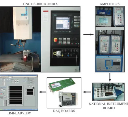
(8) 3 Intelligent Monitoring and Supervisory Control System 3.1 Introduction . . . . . . . . . . . . . . . . . . . . . . . . . . . . . . . . . . . . . . . . 3.2 Intelligent monitoring and process planning system . . . . . . . . . . . . . . . . . . . 3.3 Data Acquisition System . . . . . . . . . . . . . . . . . . . . . . . . . . . . . . . . . 3.3.1 Experimental set-up and sensors . . . . . . . . . . . . . . . . . . . . . . . . . 3.3.2 Sensors, amplifiers, and data acquisition boards . . . . . . . . . . . . . . . . . 3.3.3 Pre-processing of the signals . . . . . . . . . . . . . . . . . . . . . . . . . . . 3.3.4 Feature vectors extracted from vibration, forces, and acoustic emission signals 3.3.5 PCA Theory . . . . . . . . . . . . . . . . . . . . . . . . . . . . . . . . . . . 3.4 Analysis of the results . . . . . . . . . . . . . . . . . . . . . . . . . . . . . . . . . . .. . . . . . . . . .. . . . . . . . . .. . . . . . . . . .. . . . . . . . . .. . . . . . . . . .. . . . . . . . . .. . . . . . . . . .. 28 28 29 29 29 30 35 39 46 51. 4 Surface Roughness Monitoring Module 4.1 Introduction . . . . . . . . . . . . . . . . . . . . . . . . . . . . 4.2 Selection of the materials and test pieces for the experimentation 4.3 Test pieces for the experimentation . . . . . . . . . . . . . . . . 4.4 Measurement of the surface roughness . . . . . . . . . . . . . . 4.5 Screening factorial design . . . . . . . . . . . . . . . . . . . . . 4.5.1 Statistical analysis . . . . . . . . . . . . . . . . . . . . 4.6 Design of Experiments (DoE) . . . . . . . . . . . . . . . . . . 4.6.1 Factors and levels for the DoE . . . . . . . . . . . . . . 4.7 Modeling of the Ra using Response Surface Methodology . . . 4.7.1 RSM for the new cutting tool condition . . . . . . . . . 4.7.2 RSM for the half-new cutting tool condition . . . . . . . 4.7.3 RSM for the half-worn cutting tool condition . . . . . . 4.7.4 RSM for the worn cutting tool condition . . . . . . . . . 4.7.5 Analysis of results with the RSM models . . . . . . . . 4.8 Modeling of the Ra by using ANN . . . . . . . . . . . . . . . . 4.8.1 Input and Output variables selection . . . . . . . . . . . 4.8.2 Preprocessing of the input variables . . . . . . . . . . . 4.8.3 Training ANN Model . . . . . . . . . . . . . . . . . . . 4.8.4 Testing ANN Model . . . . . . . . . . . . . . . . . . . 4.8.5 Validation tests for the ANN models . . . . . . . . . . . 4.9 Results and contributions . . . . . . . . . . . . . . . . . . . . .. . . . . . . . . . . . . . . . . . . . . .. . . . . . . . . . . . . . . . . . . . . .. . . . . . . . . . . . . . . . . . . . . .. . . . . . . . . . . . . . . . . . . . . .. . . . . . . . . . . . . . . . . . . . . .. . . . . . . . . . . . . . . . . . . . . .. . . . . . . . . . . . . . . . . . . . . .. 52 52 52 53 54 54 56 61 61 63 65 66 67 67 67 73 73 74 76 77 78 80. . . . .. 84 84 84 86 86. 5 Cutting tool wear monitoring module 5.1 Introduction . . . . . . . . . . . . . . 5.2 Cutting tool wear condition . . . . . . 5.3 Methodology to wear the cutting tool . 5.4 Results of the tool life tests . . . . . .. . . . .. . . . .. . . . .. . . . .. . . . . ix. . . . .. . . . .. . . . .. . . . .. . . . .. . . . .. . . . .. . . . .. . . . .. . . . . . . . . . . . . . . . . . . . . .. . . . .. . . . . . . . . . . . . . . . . . . . . .. . . . .. . . . . . . . . . . . . . . . . . . . . .. . . . .. . . . . . . . . . . . . . . . . . . . . .. . . . .. . . . . . . . . . . . . . . . . . . . . .. . . . .. . . . . . . . . . . . . . . . . . . . . .. . . . .. . . . . . . . . . . . . . . . . . . . . .. . . . .. . . . . . . . . . . . . . . . . . . . . .. . . . .. . . . . . . . . . . . . . . . . . . . . .. . . . .. . . . . . . . . . . . . . . . . . . . . .. . . . .. . . . . . . . . . . . . . . . . . . . . .. . . . .. . . . . . . . . . . . . . . . . . . . . .. . . . .. . . . .. . . . .. . . . .. . . . .. . . . .. . . . ..

(9) 5.5. 5.6. 5.7. Hidden Markov Model approach . . . . . . . . . . . . . . . . . . . . . 5.5.1 Baum-Welch Algorithm . . . . . . . . . . . . . . . . . . . . . 5.5.2 Viterbi Algorithm . . . . . . . . . . . . . . . . . . . . . . . . . Monitoring and diagnosis of cutting tool wear condition . . . . . . . . . 5.6.1 Classification of the cutting tool wear condition by using HMM 5.6.2 Performance of the HMM approach . . . . . . . . . . . . . . . Analysis of the results and contributions . . . . . . . . . . . . . . . . .. . . . . . . .. . . . . . . .. . . . . . . .. . . . . . . .. . . . . . . .. . . . . . . .. . . . . . . .. . . . . . . .. . . . . . . .. . . . . . . .. . . . . . . .. . . . . . . .. . . . . . . .. . . . . . . .. . . . . . . .. 87 89 89 90 90 93 96. 6 Intelligent monitoring and process planning system 6.1 Introduction . . . . . . . . . . . . . . . . . . . . . . . . . . . 6.2 Intelligent monitoring and process planning system . . . . . . 6.2.1 Optimization process in Pre-process operating mode . 6.2.2 Optimization process in the In-process operating mode 6.3 Markov Decision Process . . . . . . . . . . . . . . . . . . . . 6.3.1 Police iteration . . . . . . . . . . . . . . . . . . . . . 6.3.2 Value iteration . . . . . . . . . . . . . . . . . . . . . 6.4 Implementation of the IMPPS . . . . . . . . . . . . . . . . . 6.5 Results . . . . . . . . . . . . . . . . . . . . . . . . . . . . . . 6.5.1 Validation with original experiments . . . . . . . . . . 6.5.2 Validation tests with new experiments . . . . . . . . . 6.5.3 Optimization in Pre-process operating mode . . . . . 6.5.4 Optimization in the In-process operating mode . . . . 6.5.5 Optimal machining policy . . . . . . . . . . . . . . . 6.6 Results and contributions . . . . . . . . . . . . . . . . . . . .. . . . . . . . . . . . . . . .. . . . . . . . . . . . . . . .. . . . . . . . . . . . . . . .. . . . . . . . . . . . . . . .. . . . . . . . . . . . . . . .. . . . . . . . . . . . . . . .. . . . . . . . . . . . . . . .. . . . . . . . . . . . . . . .. . . . . . . . . . . . . . . .. . . . . . . . . . . . . . . .. . . . . . . . . . . . . . . .. . . . . . . . . . . . . . . .. . . . . . . . . . . . . . . .. . . . . . . . . . . . . . . .. . . . . . . . . . . . . . . .. . . . . . . . . . . . . . . .. . . . . . . . . . . . . . . .. . . . . . . . . . . . . . . .. . . . . . . . . . . . . . . .. . . . . . . . . . . . . . . .. 98 98 99 100 101 101 103 104 104 106 106 106 108 111 112 120. 7 Discussion and future work 7.1 General contributions . . . . . . . . . . . . . 7.2 Specific results and contributions . . . . . . . 7.2.1 Important research results . . . . . . 7.2.2 Specific contributions of the research 7.3 Future work . . . . . . . . . . . . . . . . . . 7.4 Concluding discussion . . . . . . . . . . . .. . . . . . .. . . . . . .. . . . . . .. . . . . . .. . . . . . .. . . . . . .. . . . . . .. . . . . . .. . . . . . .. . . . . . .. . . . . . .. . . . . . .. . . . . . .. . . . . . .. . . . . . .. . . . . . .. . . . . . .. . . . . . .. . . . . . .. . . . . . .. 122 122 123 123 125 126 128. . . . . .. 137 137 138 138 139 140. A Machining Process Concepts A.1 Important variables in machining processes A.2 Surface Roughness . . . . . . . . . . . . . A.3 Tool wear in metal cutting . . . . . . . . . A.4 Mechanisms and causes in tool damage . . A.5 Machining optimization . . . . . . . . . . .. . . . . .. . . . . . .. . . . . .. x. . . . . . .. . . . . .. . . . . . .. . . . . .. . . . . . .. . . . . .. . . . . . .. . . . . .. . . . . . .. . . . . .. . . . . . .. . . . . .. . . . . . .. . . . . .. . . . . . .. . . . . .. . . . . .. . . . . .. . . . . .. . . . . .. . . . . .. . . . . .. . . . . .. . . . . .. . . . . .. . . . . .. . . . . .. . . . . .. . . . . .. . . . . .. . . . . .. . . . . .. . . . . .. . . . . .. . . . . ..

(10) A.5.1 Choice of feed . . . . . . . . . . . . . . . . . . . . . . . . . . . . . . . . . . . . . . . . . 141 A.5.2 Choice of cutting speed . . . . . . . . . . . . . . . . . . . . . . . . . . . . . . . . . . . . . 141 B Sensors, amplifiers, and data acquisition boards B.1 Introduction . . . . . . . . . . . . . . . . . . . . . . . . . . . . B.2 Accelerometers . . . . . . . . . . . . . . . . . . . . . . . . . . B.3 Acoustic Emission . . . . . . . . . . . . . . . . . . . . . . . . B.4 Amplifiers configuration . . . . . . . . . . . . . . . . . . . . . B.5 Behaviour of the process state variables in the frequency domain B.5.1 Accelerometers and dynamometers signals . . . . . . . B.5.2 Acoustic Emission signals . . . . . . . . . . . . . . . . B.5.3 MFCC computed for the process state variables . . . . .. . . . . . . . .. . . . . . . . .. . . . . . . . .. . . . . . . . .. . . . . . . . .. . . . . . . . .. . . . . . . . .. . . . . . . . .. . . . . . . . .. . . . . . . . .. . . . . . . . .. . . . . . . . .. . . . . . . . .. . . . . . . . .. . . . . . . . .. . . . . . . . .. . . . . . . . .. . . . . . . . .. . . . . . . . .. C Aluminium Alloys. 142 142 142 143 143 144 144 145 145 152. D Measurement of Ra , flank wear and run-out D.1 Procedure to measure Ra . . . . . . . . . . . . . . . . . . . . . . . . . . . . . D.2 Surface profile parameters definitions . . . . . . . . . . . . . . . . . . . . . . D.3 Methodology for assessment the surface texture . . . . . . . . . . . . . . . . . D.3.1 Parameter estimation . . . . . . . . . . . . . . . . . . . . . . . . . . . D.3.2 Evaluation length and measurement of the roughness profile parameters D.4 Measurement of the flank wear and run-out . . . . . . . . . . . . . . . . . . .. . . . . . .. . . . . . .. . . . . . .. . . . . . .. . . . . . .. . . . . . .. . . . . . .. . . . . . .. . . . . . .. . . . . . .. . . . . . .. 155 155 155 156 156 157 159. E Statistical analysis of the screening factorial design. 162. F Modeling analysis with RSM F.1 RSM for the new cutting tool condition . . . . . . . . . . . . . . . . F.2 Modeling of the Ra with RSM and half-new cutting tool condition . F.3 Modeling of the Ra with RSM and half-worn cutting tool condition . F.4 Modeling of the Ra with RSM and worn cutting tool condition . . . F.5 Modeling of the Ra by using ANN . . . . . . . . . . . . . . . . . .. . . . . .. 167 167 170 170 175 178. . . . . . . .. 179 179 181 181 182 183 183 184. G Tool-life testing procedure and parameters G.1 Tool life testing procedure . . . . . . . G.2 Methodology to wear the cutting tool . . G.2.1 Convex geometry (Big Island) . G.2.2 Concave geometry (Big Box) . G.2.3 Convex geometry (Small Island) G.2.4 Concave geometry (Small Box) G.2.5 Straight path geometry . . . . .. . . . . . . .. . . . . . . .. . . . . . . .. . . . . . . . xi. . . . . . . .. . . . . . . .. . . . . . . .. . . . . . . .. . . . . . . .. . . . . . . .. . . . . . . .. . . . . . . .. . . . . . . .. . . . . . . .. . . . . . . .. . . . . .. . . . . . . .. . . . . .. . . . . . . .. . . . . .. . . . . . . .. . . . . .. . . . . . . .. . . . . .. . . . . . . .. . . . . .. . . . . . . .. . . . . .. . . . . . . .. . . . . .. . . . . . . .. . . . . .. . . . . . . .. . . . . .. . . . . . . .. . . . . .. . . . . . . .. . . . . .. . . . . . . .. . . . . .. . . . . . . .. . . . . .. . . . . . . .. . . . . .. . . . . . . .. . . . . .. . . . . . . ..

(11) G.3 Results of the tool-life tests . . . . . . . . . . . . . . . . . . . . . . . . . . . . . . . . . . . . . . . 184 H Theory of the Markov Hidden Models H.1 Discrete Markov processes . . . . . . . . . . . . . . . . . . . . . . H.2 Extension to Hidden Markov Models . . . . . . . . . . . . . . . . . H.2.1 Baum-Welch Algorithm . . . . . . . . . . . . . . . . . . . H.2.2 Viterbi Algorithm . . . . . . . . . . . . . . . . . . . . . . . H.3 Monitoring and diagnose the cutting tool wear condition . . . . . . H.3.1 Assessment of the cutting tool wear condition by using ANN H.4 Conclusions . . . . . . . . . . . . . . . . . . . . . . . . . . . . . . I. . . . . . . .. . . . . . . .. . . . . . . .. . . . . . . .. . . . . . . .. . . . . . . .. . . . . . . .. . . . . . . .. . . . . . . .. . . . . . . .. . . . . . . .. . . . . . . .. . . . . . . .. . . . . . . .. . . . . . . .. . . . . . . .. . . . . . . .. 188 188 189 191 191 192 192 194. Machining cost. 196. J List of publications. 200. xii.

(12) Nomenclature Variable. Description. Units. A Ai,j Acc Accx,sp Accx Accy,sp Accz,sp Accx,wp Accy,wp a a ae ap ap a1 a2 a1,..,4 B b b C CC Coef Curv c DF Dtool. Finite set of actions of the operator The state transition probability distribution Acceleration X-direction acceleration in the spindle Acceleration in the x − axis of the workpiece Y-direction acceleration in the spindle Z-direction acceleration in the spindle X-direction acceleration in workpiece Y-direction acceleration in workpiece Number of levels of the factors High of the island/box Radial depth of cut Axial depth of cut Axial depth of cut Minimum high of the box geometry Maximum high of the box geometry Actions of the operator The observation symbol probability distribution Chip width Width of the island/box base Concave path Cutting conditions Coefficients in the multiple regression Curvature of the machined path Cepstrum coefficient number Degrees of freedom Diameter of the cutting tool. xiii. – – m/s2 m/s2 – m/s2 m/s2 m/s2 m/s2 – mm mm mm mm mm mm – – mm mm – – – mm−1 – – mm.

(13) Variable E ei F Fy f f fHz fM el fz HB I k L Lt l lc M ME M F CC M SE M Sl evels N N N Nf Np Ns n n nc nc nF P P PC PG p. Description. Units. Absolute error Represent the ith Eigenvector Statistical F distribution Force in the y − axis of the workpiece Instantaneous Cost function Feed Real frequency scale Perceive Mel frequency scale Feed per tooth Hardness of the workpiece Convex path Number of factors Evaluation length Length of the arc/line defined by the geometry path Sampling length Length of the cut Number of distinct observation symbols per state Average percentage error Mel Frequency Cepstrum Coefficient Mean square value of the errors Mean square value of the levels Number of states considered in S Number of samples Total number of observations Number of samples in a short frame Number of filters Number of states in the HMM Spindle speed Number of replicates Number central runs in the DoE Number of cycles of the cutting tool edge Number of runs in the DoE Defines the state transition probability distribution function Principal components vector Cutting parameters Geometric parameters Defines the number of components xiv. – – – N – mm/rev Hz Mels mm/tooth BHN – – mm mm mm mm – % – (µm)2 (µm)2 – – – – – – rpm – – – – – – – –.

(14) Variable p − value qt R R R Ra 0 Ra Rad Rad Ra,avg Ra,measured Ra,meas Ra,min Rap Ra,pred Rap Ra,obs Rpath Rq RSm Rsk Rt Rtool Rt Rz r re S S SE SSR SSE SST St T Tc. Description. Units. Probability to reject the null hypothesis Represents the state at time t Curvature radio Radio of the concave/convex path Reward function Surface Roughness or arithmetic average roughness Predicted Ra Desired Surface Roughness Desired surface roughness Average value of Ra Surface roughness measured Measurement of surface roughness Minimum surface roughness Predicted Surface Roughness Prediction of surface roughness Predicted surface roughness Observed surface roughness Radio of the geometry path Root mean square value of the Z values within a sampling length Mean value of the profile element widths (Xs) Skewness The maximum peak to valley height Radio of the cutting tool Sum of Zp and Zv within the evaluation length Sum of Zp and Zv within the sampling length Interest rate Cutter nose radius Finite set of states in the machining process Defines the state space Estimated standard error Explained variation or the regression sum of squares Unexplained variation or the error sum of squares Total sum of squares Final length of the convex/concave arc Data set matrix to compute the PCA Total cutting time of the cutting tool. – – mm mm – µm µm µm µm µm µm µm µm µm µm µm µm mm µm µm – µm mm µm µm – mm – – – (µm)2 (µm)2 (µm)2 mm – min. xv.

(15) Variable. Description. Units. T − test te tm s1,..,4 V VB V B1 V B2 V B3 V Bmax vc vf V ol VB vc vf vp X X, Y, Z Xs x x̄ Y ȳ Z z z̄ Zp Zv α α β 0 β ε λc λ µ. Statistics value to evaluate the difference in means of the Coef Cutting edge time Machining time Defines a specific state of the cutting tool Defines the symbols space in the HMM Flank wear land in the cutting tool edge Wear land extended over the tool flanks of the active cutting tool Wear land with irregular width in the cutting tool edge Exaggerated and localized form of wear at specific part of the flank Maximum wear land in the cutting tool edge and it is equal to V B3 Cutting speed Feed rate Volume of the removal metal Flank wear in the cutting tool edge Cutting speed Feed rate Vector of process state variables Energy of the spectrum Milling machine axes Distance between peak to peak (width) Amplitude of the signal Mean value of a specific input variable Scaled energy of the spectrum Normalized input variable, with mean zero and σ = 1 Absolute ordinate value within a sampling length Number of tooth of the cutting tool Bipolar sigmoidal input variable Height of the largest profile peak Height of the largest profile valley Major cutting edge angle Distance of the axial runs from the design center. Helix angle of the cutting tool End cutting edge angle Residual error Cutoff value Eigenvalue Dimensional mean vector xvi. – min min – – mm mm mm mm mm m/min mm/min mm3 mm m/min mm/min – – µm Volts – – µm – – µm µm Degrees – Degrees Degrees – mm – –.

(16) Variable φi Σ χ ωN ξ ξ¯ σ ∆φ λ π ∆Error β π ∆Error α ν. Description. Units th. Triangular weighted function, associated with the i filter Covariance matrix Logarithm value of the energy spectrum Constant equal to e(−2πi)/N Represents any value of the factors Normalized value of the factors Standard deviation of the predicted response Immersion angle of the cutting tool Defines the representation of the HMM Initial state distribution in the HMM Absolute percent error between the predicted and desired Ra Vector that maps the state space into the action space A stationary policy that can be defined by an action function Absolute percent error between the predicted and desired Ra Discount factor Expected total discount cost. xvii. – – – – – µm rad – – – – – – – –.

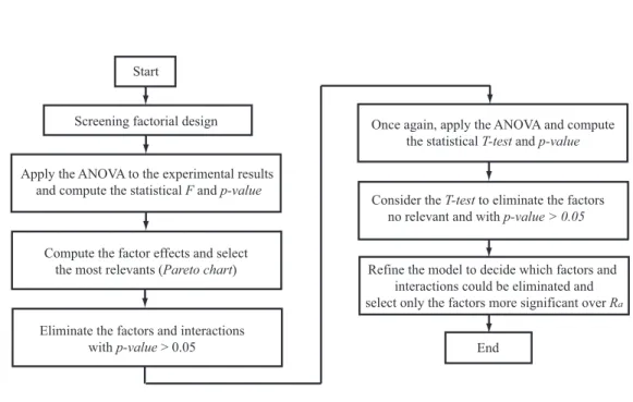
(17) List of Figures 1.1. Diagram of the intelligent monitoring and supervision system . . . . . . . . . . . . . . . . . . . . .. 2.1 2.2 2.3 2.4 2.5 2.6. Main components and movements of the vertical milling machine . . . . . . . . . The face and peripheral milling are basic geometric modes of milling operations . . Surface shape after the machining process with different imperfections. . . . . . . Idealized model of surface roughness for a cutting tool . . . . . . . . . . . . . . . Several areas of the cutting tool that present wear during the metal cutting process. Classification of the factors that affect the Ra of a workpiece . . . . . . . . . . . .. . . . . . .. . . . . . .. . . . . . .. . . . . . .. 10 10 11 12 13 14. 3.1 3.2 3.3 3.4 3.5 3.6 3.7 3.8 3.9 3.10 3.11 3.12 3.13 3.14 3.15 3.16. An intelligent monitoring and supervisory control system can provide cost effective control . . Experimental set-up: CNC machining center, amplifiers, DAQ boards, and LabView program. The Data Acquisition System is shown with the different sensors . . . . . . . . . . . . . . . . The accelerometers and acoustic emission sensors were fixed in a ring . . . . . . . . . . . . . Process signals recorded during the cutting process with fresh cutting tool . . . . . . . . . . . Power spectral density (P SD) plots in the frequency domain of the signals . . . . . . . . . . Power spectral density (P SD) plots in the frequency domain of specific signals . . . . . . . . AE-signals recorded with different sampling rate . . . . . . . . . . . . . . . . . . . . . . . . Power spectral density (PSD) of the AE signals . . . . . . . . . . . . . . . . . . . . . . . . . AE Signals in the time domain and Power spectral density of AE-signals . . . . . . . . . . . . The plots depict the power spectral density for the AE . . . . . . . . . . . . . . . . . . . . . . Feature extraction process . . . . . . . . . . . . . . . . . . . . . . . . . . . . . . . . . . . . MFCC computed from the acceleration (Accy ) process signal . . . . . . . . . . . . . . . . . . The MFCC computed from the acceleration (Accy ) process signal and the cutting conditions . The MFCC computed from the acoustic emission (AE spindle) process signal . . . . . . . . . The plots show the scores of the original data . . . . . . . . . . . . . . . . . . . . . . . . . .. . . . . . . . . . . . . . . . .. . . . . . . . . . . . . . . . .. . . . . . . . . . . . . . . . .. 30 31 32 33 36 37 38 39 40 41 42 44 45 47 48 50. 4.1 4.2 4.3. Test pieces designed for the experimentation with concave and convex paths . . . . . . . . . . . . . Test pieces used for the experimentation with the straight path. . . . . . . . . . . . . . . . . . . . . Example of the obtained profile from the Ra measurements with the Surfcom type 130A . . . . . .. 53 54 55. xviii. . . . . . .. . . . . . .. . . . . . .. . . . . . .. . . . . . .. 7.

(18) 4.4 4.5 4.6 4.7 4.8 4.9 4.10 4.11 4.12 4.13 4.14 4.15 4.16 4.17. Flow diagram to select the most relevant factors over Ra in the screening analysis. . . . . . . Pareto chart of the standardized effects . . . . . . . . . . . . . . . . . . . . . . . . . . . . . . The eight factors are shown with the main effects plot for Ra in the upper plot . . . . . . . . . Representation of the central composite designs for k = 2 and k = 3 factors . . . . . . . . . . Validation of the used information to build the Statistical Model with new cutting tool . . . . . The plots depict the quadratic behaviour of the response Ra as a function of the defined factors (A) These plots show the effects of fz and Dt ool on Ra . . . . . . . . . . . . . . . . . . . . . Contour plot to show the effects of fz and DT ool on Ra for all cutting tool conditions . . . . . Comparison of the results of the RSM model with two mechanistic models . . . . . . . . . . . Comparison of the measured Ra versus estimated Ra value . . . . . . . . . . . . . . . . . . . Proposal architecture for the ANN model with the inputs and outputs variables . . . . . . . . . The plot depicts two experiments with different cutting and geometric parameters . . . . . . . Comparison of the Ra values obtained from the DoE with: (a) ANN model . . . . . . . . . . . Comparison of the Ra values which were observed from new experiments . . . . . . . . . . .. . . . . . . . . . . . . . .. . . . . . . . . . . . . . .. . . . . . . . . . . . . . .. 58 59 62 64 66 68 69 70 71 72 75 75 80 82. 5.1 5.2 5.3 5.4 5.5 5.6 5.7 5.8 5.9 5.10 5.11. The figure shows the area, where the flank wear is located . . . . . . . . . . . . . . . . . Evolution of flank wear on the cutting edges . . . . . . . . . . . . . . . . . . . . . . . . Evolution of the maximum value of flank wear on the cutting edges . . . . . . . . . . . Procedure for computing the approach performance . . . . . . . . . . . . . . . . . . . . Flow diagram for monitoring and diagnosis of the cutting tool wear condition . . . . . . Number of iterations required to compute the HMM parameters . . . . . . . . . . . . . . Evaluation of the HMM performance with the testing data set and different configurations Evaluation of the HMM performance using different process state variables . . . . . . . Performance of the HMMs with 10 runs and different process signals . . . . . . . . . . . Performance of the HMM with the MFCC computed with Hamming window, 40 filters . Evaluation of the misclassification percentage in FFR conditions . . . . . . . . . . . . .. . . . . . . . . . . .. . . . . . . . . . . .. . . . . . . . . . . .. . . . . . . . . . . .. . . . . . . . . . . .. . . . . . . . . . . .. 85 87 88 90 92 93 94 94 95 96 97. 6.1 6.2 6.3 6.4 6.5 6.6 6.7 6.8 6.9. Flow diagram of the IMPPS . . . . . . . . . . . . . . . . . . . . . . . . . . . . . . . . . Flow diagram for the intelligent monitoring, diagnostic of cutting tool condition . . . . . . Test pieces 01, 02, and 03 with machining geometries, straight, concave and convex paths. Comparison between the measured and estimated Ra values by using (a) RSM, (b) ANN . Evaluation of optimum cutting parameters with GA in Pre-process operating mode . . . . Evaluation of the optimum cutting parameters with GA in Pre-process . . . . . . . . . . . Evaluation of the optimum cutting parameters with GA in Pre-process . . . . . . . . . . . Simulation of the Markov system . . . . . . . . . . . . . . . . . . . . . . . . . . . . . . . Comparison of costs for the different actions versus the optimal policy . . . . . . . . . . .. . . . . . . . . .. . . . . . . . . .. . . . . . . . . .. . . . . . . . . .. . . . . . . . . .. 99 105 107 111 112 113 114 118 119. A.1 Behavior of the tool damage mechanisms as a function of the cutting temperature and removal rate. 139 A.2 Different costs for a typical machining operation . . . . . . . . . . . . . . . . . . . . . . . . . . . 141. xix.

(19) B.1 B.2 B.3 B.4 B.5 B.6 B.7 B.8 B.9 B.10. Frequency domain of specific signals for the experiment number 07 Frequency domain of specific signals for the experiment number 10 Frequency domain of specific signals for the experiment number 25 Frequency domain of specific signals for the experiment number 17 Experiment number 07. Power spectral density for the AE signals . Experiment number 10. Power spectral density for the AE signals . Experiment number 25. Power spectral density for the AE signals . Experiment number 17. Power spectral density for the AE signals . MFCC computed from the cutting force . . . . . . . . . . . . . . . MFCC computed from the acoustic emission . . . . . . . . . . . .. . . . . . . . . . .. . . . . . . . . . .. . . . . . . . . . .. . . . . . . . . . .. . . . . . . . . . .. . . . . . . . . . .. . . . . . . . . . .. . . . . . . . . . .. . . . . . . . . . .. . . . . . . . . . .. . . . . . . . . . .. . . . . . . . . . .. . . . . . . . . . .. . . . . . . . . . .. . . . . . . . . . .. . . . . . . . . . .. . . . . . . . . . .. 146 146 147 147 148 148 149 149 150 151. D.1 D.2 D.3 D.4 D.5 D.6 D.7. Main parts of the portable Surfcom type 130A. . . . . . . . . . . . . . . . . . . . . . . . . . . Identification of the proposal areas for assessment the profile parameters . . . . . . . . . . . . . Identification of the sections for measuring the Ra over the machined surface . . . . . . . . . . Assessment of the surface roughness: (a) Measurement with the stylus tip of the Surfcom 130A Equipment for measuring the flank wear of the cutting edge. . . . . . . . . . . . . . . . . . . . Evolution of the flank wear for the 10 mm cutting tool. . . . . . . . . . . . . . . . . . . . . . . Assessment of the radial runout of the cutter edges. The cutting tool diameter is 20 mm. . . . . .. . . . . . . .. . . . . . . .. 157 157 159 159 160 161 161. E.1 (a)The seven factors considered with the main effects plot for Ra . (b) Interactions plot for Ra . . . . 165 F.1 F.2 F.3. Validation of the used information to build the Statistical Model . . . . . . . . . . . . . . . . . . . 170 Validation of the used information to build the Statistical Model . . . . . . . . . . . . . . . . . . . 175 Validation of the used information to build the Statistical Model . . . . . . . . . . . . . . . . . . . 178. G.1 Machining of the convex geometry. . . . . . . . . . . . . . . . . . . . . . . . . . . . . . . . . . . . 181 G.2 Machining of the concave geometry. . . . . . . . . . . . . . . . . . . . . . . . . . . . . . . . . . . 183 H.1 (a) HMM with one coin and two states. (b) HMM with two coins . . . . . . . . . . . . . . . . . . . 190 H.2 ANN model implemented for monitoring and diagnosis the on-line cutting tool condition. . . . . . . 193 H.3 Monitoring and Diagnosis the cutting tool condition with the ANN(12,12,1) model . . . . . . . . . 195. xx.

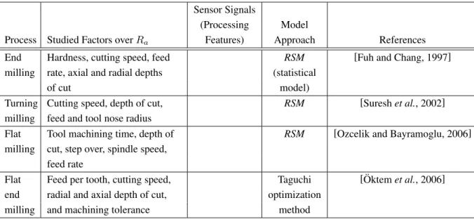
(20) List of Tables 2.1 2.2 2.3 2.4 2.5 2.6. Machine theory approach . . . . . . . . . . . . . . . . . . . . . . . . . . . Experimental approach . . . . . . . . . . . . . . . . . . . . . . . . . . . . Design of experiments approach . . . . . . . . . . . . . . . . . . . . . . . Artificial Intelligence approach . . . . . . . . . . . . . . . . . . . . . . . . Comparison of different research efforts in cutting tool condition monitoring Summary of the optimization research works in the machining process. . .. . . . . . .. . . . . . .. . . . . . .. . . . . . .. . . . . . .. . . . . . .. . . . . . .. . . . . . .. . . . . . .. . . . . . .. . . . . . .. . . . . . .. . . . . . .. 19 21 22 22 23 26. 3.1 3.2 3.3 3.4. Workpiece materials and cutting tools . . . . . . . . . . . . . . . . Characteristics of the sensors installed on the CNC machining center Cutting conditions of the selected experiment . . . . . . . . . . . . Parameters to characterize the surface roughness of the test pieces .. . . . .. . . . .. . . . .. . . . .. . . . .. . . . .. . . . .. . . . .. . . . .. . . . .. . . . .. . . . .. . . . .. 31 33 36 49. 4.1 4.2 4.3 4.4 4.5 4.6 4.7 4.8 4.9 4.10 4.11 4.12 4.13 4.14 4.15 4.16. Aluminium Alloys selected for the experimentation. . . . . . . . . . . . . . . . . . . . . . . . . . . Factors and levels defined for the screening design. . . . . . . . . . . . . . . . . . . . . . . . . . . Design of experiments for the screening design stage and the measurement of Ra . . . . . . . . . . Analysis of Variance for Ra (coded units). . . . . . . . . . . . . . . . . . . . . . . . . . . . . . . . Estimated effects and coefficients for Ra (coded units) . . . . . . . . . . . . . . . . . . . . . . . . Analysis of Variance for Ra (coded units) . . . . . . . . . . . . . . . . . . . . . . . . . . . . . . . Factors and levels of the experimentation. . . . . . . . . . . . . . . . . . . . . . . . . . . . . . . . The experiments for the central composite design (half fraction) . . . . . . . . . . . . . . . . . . . Average percentage error between the measured and estimated Ra values with different models. . . Cutting parameters and conditions for the new experiments. Also, it is included the results of the Ra . Architecture of the ANN models used to compute the Ra . . . . . . . . . . . . . . . . . . . . . . . . Performance of the ANN models for the training data set . . . . . . . . . . . . . . . . . . . . . . . Performance of the ANN models for the testing data set . . . . . . . . . . . . . . . . . . . . . . . . Selected experiments with measured and estimated Ra values . . . . . . . . . . . . . . . . . . . . . Cutting conditions and geometric parameters defined for the new experiments . . . . . . . . . . . . Results of the estimated Ra with the ANN models . . . . . . . . . . . . . . . . . . . . . . . . . . .. 53 55 57 59 61 63 65 65 73 74 76 77 78 79 80 81. xxi. . . . .. . . . .. . . . .. . . . ..

(21) 5.1. Cutting tool wear condition and the flank wear observed during the experimentation. . . . . . . . .. 6.1 6.2 6.3 6.4 6.5 6.6 6.7 6.8 6.9 6.10. Experiments selected with the measured and estimated Ra values . . . . . . . . . . . . . . . . . . Test pieces with the cutting conditions, and geometric parameters defined for the new experiments. Results of the estimated Ra in Pre and In-process operating mode . . . . . . . . . . . . . . . . . Optimal cutting conditions to minimize the Ra in Pre-process condition (7075 Aluminium alloy). Evaluation of Ra with new cutting conditions . . . . . . . . . . . . . . . . . . . . . . . . . . . . Optimal cutting conditions to minimize the Ra in Pre-process condition (6082 Aluminium alloy). Experiments used to validate the optimization process during the In-process operating mode. . . . Results computed with the Policy Iteration algorithm. . . . . . . . . . . . . . . . . . . . . . . . . Results computed with the Value Iteration algorithm. . . . . . . . . . . . . . . . . . . . . . . . . Comparison of the applied cost for 6082 − T 6 workpiece material and 16 mm . . . . . . . . . . .. . . . . . . . . . .. 107 108 109 110 110 113 115 117 117 120. B.1 B.2 B.3 B.4. Nexus amplifier configuration for the two DeltaTron channels (4) . . . . . Parameters defined to configure the Kistler charge amplifier type 5011 . . . Configuration parameters for the multi-channel amplifier type 5070. . . . . Cutting conditions for the experiments 07, 10, 25 and 17 (second replicate).. . . . .. 144 144 145 145. . . . .. . . . .. . . . .. . . . .. . . . .. . . . .. . . . .. . . . .. . . . .. . . . .. . . . .. . . . .. 87. D.1 Roughness sampling lengths for the measurement of Ra for non-periodic profiles. . . . . . . . . . . 158 D.2 Roughness sampling lengths for the measurement of Rz for non-periodic profiles. . . . . . . . . . . 158 D.3 Assessment of the radial runout of the cutting tool edges . . . . . . . . . . . . . . . . . . . . . . . 160 E.1 E.2 E.3 E.4 E.5 E.6. Estimated effects and coefficients for Ra with vc eliminated (coded units). . . . . . . Analysis of Variance for Ra with Vc eliminated (coded units). . . . . . . . . . . . . Estimated effects and coefficients for Ra with ap eliminated (coded units). . . . . . . Analysis of Variance for Ra with ap eliminated (coded units). . . . . . . . . . . . . Estimated effects and coefficients for Ra with Dtool and ae eliminated (coded units). Analysis of Variance for Ra with Dtool and ae eliminated (coded units). . . . . . . .. . . . . . .. . . . . . .. . . . . . .. . . . . . .. . . . . . .. . . . . . .. . . . . . .. . . . . . .. 163 163 164 164 166 166. F.1 F.2 F.3 F.4 F.5 F.6 F.7 F.8. Values of the considered factors for the experiments, and the measurements of the parameters 2 Results of the ANOVA analysis: R2 = 0.906, Radj = 0.895 with 128 runs . . . . . . . . . . Factors considered for the experiments, and the measurements of the parameters . . . . . . . 2 Results of the ANOVA analysis: R2 = 0.9, Radj = 0.887 . . . . . . . . . . . . . . . . . . . Factors considered for the experiments, and the measurements of the parameters . . . . . . . 2 = 0.916 with 128 runs . . . . . . . . . . Results of the ANOVA analysis: R2 = 0.927, Radj Factors considered for the experiments, and the measurements of the parameters . . . . . . . 2 Results of the ANOVA analysis: R2 = 0.934, Radj = 0.925 with 128 runs . . . . . . . . . .. . . . . . . . .. . . . . . . . .. . . . . . . . .. . . . . . . . .. 168 169 171 172 173 174 176 177. G.1 Recommended cutting conditions for end milling. . . . . . . . . . . . . . . . . . . . . . . . . . . . 180 G.2 Minimum limits of cutting conditions. . . . . . . . . . . . . . . . . . . . . . . . . . . . . . . . . . 180 xxii.

(22) G.3 Tool-life parameters for the experiments with 6082 − T 6 Aluminium alloy . . . . . . . . . . . . . . 185 G.4 Evolution of the flank wear during the experimentation . . . . . . . . . . . . . . . . . . . . . . . . 186 G.5 Evolution of the flank wear during the experimentation . . . . . . . . . . . . . . . . . . . . . . . . 187 H.1 Tool-wear from ANN model is mapped with the cutting tool wear condition. . . . . . . . . . . . . . 194 H.2 Performance of the ANN model with the training and testing data sets . . . . . . . . . . . . . . . . 194 I.1 I.2 I.3 I.4 I.5 I.6 I.7 I.8. Time constants obtained during the experimentation, and used to compute the cost functions. List of the cost required to compute the cost functions. . . . . . . . . . . . . . . . . . . . . Operation cost for the a1 action. . . . . . . . . . . . . . . . . . . . . . . . . . . . . . . . . Cost for the decision theory. Actions a1 and a2 . . . . . . . . . . . . . . . . . . . . . . . . . Total cost required to compute the a1 cost function. . . . . . . . . . . . . . . . . . . . . . . Total cost required to compute the a2 cost function. . . . . . . . . . . . . . . . . . . . . . . Decision theory cost for the a3 action. . . . . . . . . . . . . . . . . . . . . . . . . . . . . . Total cost required to compute the a3 cost function. . . . . . . . . . . . . . . . . . . . . . .. xxiii. . . . . . . . .. . . . . . . . .. . . . . . . . .. . . . . . . . .. 196 197 198 198 198 198 199 199.

(23) Chapter 1. Introduction In the world, machining processes (turning, milling, and drilling) are the most widespread metal shaping processes in mechanical manufacturing. Machine tools are essential for reproducing the technologies required in an industrial economy. Currently, worldwide investment in metal-machining machine tools holds steady or continues to increase year after year, [Childs et al., 2000], for the following reasons: 1. The metal machining is capable of high precision: part tolerances of 50 µm and surface finish of 1 µm are readily achievable. 2. The machining process is very versatile: complicated free-form shapes with many features, over a large size range, can be made more cheaply, quickly, and simply by controlling the path of a standard cutting tool rather than by investing considerable time and cost in making a dedicated moulding, forming or die casting tool. 3. Also, the mechanical micro-machining has been defined as an important and relevant process owing to its ability to fabricate micro parts out of a greater range of materials and with more varied geometry than is possible with lithography and etching. Next-Generation Manufacturing refers to the application of new concepts, models, methodologies, and information technologies, with the goal of preparing manufacturing companies to become more competitive in a global and networked environment, [Molina et al., 2005]. Then, one important characteristic of future manufacturing equipment will be its ability to adapt to changing environments and conditions. This implies the opportunity to build an intelligent machine to achieve a goal or keep the performance under stochastic process conditions. An intelligent system must posse basic features and capabilities such as sensory perception, pattern recognition, learning and knowledge acquisition, inference from incomplete information, and adaptation. For these reasons, the great economies of the world want to lead production and technology in machining centers, and during the last decades, research and development has been conducted in three areas: • Advances in machine tools (machine technology) 1.

(24) 2 • Organization of machining (manufacturing systems) • The cutting edge (materials technology). 1.1 Motivation Given the importance of machining to most industries, and in order to keep the competitive edge and satisfy various customer needs, innovative manufacturing techniques have to be developed by further integration of information and manufacturing technology. In summary, through different research, several opportunities areas have been identified for present and future industrial applications. These areas are related to the following items: 1. Modelling of machining operations are relevant to improve the machining performance, workpiece quality, and attaining high productivity and/or low production cost. The use of more than one sensor for monitoring the process gives more interesting features to model the process. These systems are called multi-sensors systems, and the information acquired will be combined in order to get a sensor fusion. 2. Monitoring of the machining processes is very important in order to achieve safety, prevent fatal damage, and prevent rejects. In [Tönshoff et al., 1988] it was demonstrated that the effective machining time of the machine tool was increased from 10 % to 65 % by using a monitoring system. Then, is a great opportunity to contribute with a cutting tool condition monitoring system in order to reduce operating cost. 3. Optimization and process modelling are two important issues in the metal cutting process because the machining process is variable owing to multiple factors (e.g. cutting tool-wear, vibrations, and other disturbances). In a CNC machining center the selection of the optimal cutting parameters is important to reduce the costs and allow high product quality. Also, control strategies are very important in the optimization process and machining operations. Two kinds of control approach are identified, i.e. on-line and off-line control. Adaptive control is a kind of on-line control, and it is applied for time-varying systems with large uncertainty concerning the process dynamic characteristics and disturbances. The on-line control received much attention in the 1970s and 1980s, [van Luttervelt and Peng, 1999]. However, at that time, knowledge of metal cutting was not sufficient, an accurate tool wear model was not available, and sensor and computer technology was not developed far enough. Currently, successful development and implementation of process monitoring and control demands high flexibility of the machine tool controller and open architecture controls in the CNC machining center, [Liang et al., 2004]. To date, various transducers, signal processing schemes, control strategies, and actuators have been proposed and extensively investigated. In the area of machining process sensing, research has focused primarily on the monitoring of tool condition, chatter and part quality. Nowadays, the machining processes with high speed (HSM) is one of the modern technologies, which in comparison with conventional cutting enables to increase efficiency, accuracy, and quality of workpieces and at the same time to decrease costs and machining time. Major advantages of HSM are reported as: high material removal.

(25) Introduction. 3. rates, the reduction in lead times, low cutting forces, reduced number of technological operations, less workpiece distortion and increased precision of the part, [Cus et al., 2007]. The HSM is being mainly used in three industry sectors owing to their specific requirements: • The first industry sector deals with machining aluminium to produce automotive components, small computer parts, or medical devices. This industry needs fast metal removal, because the technological process involves many machining operations. • The second sector is aircraft industry which involves machining of long aluminium parts by removing a great amount of material from prismatic block, [de Lacalle Marcaide et al., 2004]. • The third industry sector is the die mould industry which requires dealing with finishing of hard materials. In this category is important to machine with high speed and to keep high accuracy. The HSM is the result of numerous technical advances ensuring that milling has become faster conventional milling and has gained importance as a cutting process. This implies to define a new paradigm: it is important to maximize the metal removal rate, minimize the cutting tool-wear rate and maintain the surface quality and dimensional precision of all the machined parts in HSM. Also, in several researches [Liang et al., 2004], [Narita et al., 2004], and [Erol et al., 2000] define the future of the machine tools as follows: • The machine tool must be a smart machine with the capacity to develop intelligent functions to enhance the manufacturing process. • The machine tool must be available to realize the effective, reliable, and superior manufacturing system. • New development and technology must be conducted in the process level. The process level is related to the phenomena that occurs in the interaction of the cutting tool and workpiece. To evaluate and implement these considerations in a machine tool, it is first important to define: What does an intelligent machine mean? Intelligent machine, as defined by [Haber et al., 1998], is a computationally efficient procedure combining one or more intelligent techniques (ANN, fuzzy logic, etc.) and expert criteria (e.g. operator knowledge) with one or more higher resolution levels, which basically manipulate cutting conditions (spindle speed, feed, etc.) and should be monitoring tool status and finished surface quality, as well as increasing productivity through higher metal removal rate.. 1.2 Problem description In agreement with the previous section, the following problems can be found in the industry of the metal cutting processes..

(26) 4 1. The HSM defines new concepts and strategies of the mechanical design, the design of new related frameworks with the monitoring, control, and supervision of the machining process. Furthermore, the selection of the optimal machining parameters is important for the operation of the HSM. Currently, for conventional machining there is enough information (e.g., machining databases, handbooks) to select the proper cutting parameters for specific cutting tools and workpiece materials. However, for HSM there is no available information to select the cutting parameters, so the heuristic operation is exploited based on the operator’s experience. Cutting parameters based on estimations have a direct impact on the metal cutting economics. High operating costs, low productivity, and poor quality of the product result from non-optimal cutting conditions, where there is a great opportunity to develop new models that can be integrated with optimization techniques for computing optimal cutting parameters in HSM. 2. The quality concept implies keeping consistent tolerances in the dimensional precision and the surface finish of the parts. For this reason, the surface roughness (Ra ) has received great attention in the metal cutting process. Several research works have been developed to predict the Ra and monitor the cutting tool condition In-process operating mode. However, the experimentation made in the majority of these works over Ra and flank wear (V B) only consider a specific combination of cutting tool and workpiece material. Therefore, several authors have pointed out the importance of building databases with information of different materials and cutting tools for a complete domain in the machining process. 3. In [Rehorn et al., 2005] it is mentioned that the amount of down time owing to cutter breakage on an average machine is between 6.8 % and 20 %. Even if the tool does not break during machining, the use of dull or damaged cutters can put extra strain on the machine tool and cause a loss of quality in the workpiece. It is very much appreciated that cutting tool condition monitoring system optimizes the operating cost with the same quality of the product. 4. There is a need to design and develop an intelligent monitoring and process planning system that allows the prediction of the Ra and recommends the optimal cutting condition, Pre-process, and In-process operating mode. Also, it must be available to recommend optimal policy to operate the CNC with minimum cost.. 1.3 State of the art This section presents only a short description of the main research studies related with the optimization processes, surface roughness, and cutting tool wear. Chapter 2 presents a general classification of the different techniques and methodologies used to model the surface roughness and to predict the cutting tool wear condition in machining processes.. 1.3.1 Optimization systems Optimization techniques in metal cutting processes are essential to respond to serious competition and increasing demand for quality product in the market. In [Mukherjee and Ray, 2006] a review of optimization techniques in.

(27) Introduction. 5. metal cutting processes is presented, and a general framework for process parameter optimization is discussed. Some applied optimization methods are the Taguchi method, response surface methodology, mathematical iterative search algorithm, Genetic Algorithms, and simulated annealing. Furthermore, different objective functions used in the optimization of the machining conditions include: minimum production cost, maximum production rate, increase tool life, maximum profit rate, and weighted combination of several objective functions. Cutting constraints that should be considered in machining economics include: tool-life constraint, cutting force constraint, power, chiptool interface temperature constraint, and surface finish constraint. A complete classification of the optimization techniques will be discussed in Chapter 2.. 1.3.2 Surface roughness Surface roughness (Ra ) has received serious attention for many years. It has been an important design feature and quality measure in many situations, such as parts subject to fatigue loads, precision fits, fastener holes and esthetic requirements. Some geometric models to represent the surface roughness have been developed, and they take into consideration certain aspects from the theory of machining such as process kinematics, cutting tool properties, chip formation mechanism, etc.. Other research works are based on multiple regression analysis, where the obtained models allow the prediction of the Ra as a function of different factors, such as feed rate, spindle speed, depth of cut, tool nose radius, vibration, hardness, etc.. These models are applied only for a specific combination of cutting tool and workpiece material. Systematic methods, concern with the planning of experiments, collection and analysis of data are the Response Surface Methodology and Taguchi techniques. These are used for Design of Experiments (DoE), and they are the most wide spread methodologies for the Ra prediction problem and optimization process. Also, a number of studies on the application of Artificial Intelligence (AI) have been applied in CNC machining for determining optimum cutting parameters and for modelling the Ra . These AI techniques have been used to minimize machining errors such as tool breakage, tool wear, and surface roughness.. 1.3.3 Cutting tool wear Tool wear is defined as a gradual loss of tool material at workpiece material and tool contact zones. The monitoring of cutting tool states may be classified into direct and indirect methods. Several works related with the indirect monitoring of the cutting tool wear are based on techniques such as Artificial Neural Networks (ANN), Bayesian networks (BN), multiple regression approaches, and stochastic methods. At the feature extraction level, the most frequently used techniques are the computation of average values or trends, power values in spectral bands, or statistical features. The Tool Condition Monitoring (TCM) system must include applications where prior knowledge or cutting data could not exist. Artificial intelligence, ANNs, fuzzy logic systems, and Genetic Algorithms should be some options to solve this situation..

(28) 6. 1.4 Research objectives HSM represents a modern technology which is used in important industry sectors, such as, automotive industry for machining aluminium components, the aircraft industry for machining aluminium parts, and the die mould industry which requires high surface finishing and high dimensional precision. relevant researches have been reported in this field with important advances in the following areas: 1. In optimization processes, applied models are based on Taguchi methods, and response surface methodology, and using Genetic Algorithms, and simulated annealing, the optimal cutting parameters are computed by considering different objective functions (i.e., minimum production cost, maximum production rate, maximum tool-life). However, there is a great opportunity to design and implement intelligent monitoring systems and process planning systems in HSM. 2. In surface roughness, several models have been developed (mechanistic, statistical, etc.) to estimate the Ra as function of different factors. However, they have been only applied at specific combination of workpiece and cutting tool. The cutting tool wear condition has not been considered in the models. 3. The monitoring of the cutting tool wear condition also presents important researches using Artificial Intelligence techniques for indirect monitoring of cutting edge. It is necessary to improve models to estimate the cutting tool wear condition by considering new feature extraction from different process state signals and increasing the performance of models for recognizing different states of the cutting tool wear condition. The general scope of this research is defined as: Design and implement an intelligent monitoring and supervisory control system for peripheral milling process in high speed machining. The system must compute the optimum cutting parameters as a function of a merit variable. Also, the system must allow the monitoring of the cutting tool wear condition and the surface roughness during the machining process. Figure 1.1 shows the proposal architecture with the blocks required to develop the different functions of the system. The main objectives of this research are: 1. Design and implement an intelligent monitoring and process planning system in peripheral milling process for HSM. The proposal implies to use a multi-sensor system in the CNC machining center for recording several process state variables (i.e., forces, vibration, and acoustic emission) during the machining process. Statistical and artificial intelligence techniques must be applied to integrate an intelligent system and build new models for monitoring and diagnosing the surface quality and the cutting tool wear condition. 2. Implement new models to estimate the surface roughness (Ra ) by considering several aluminium alloys, cutting parameters, geometries, and cutting tools. The most relevant factors that affect the Ra must be selected, and the Design of Experiments must be defined with the objective of building a model for covering a machine domain with the aforementioned considerations. 3. Predict the optimal cutting parameters Pre and In-process operating mode for maintaining the surface roughness quality. With the statistical models and using artificial intelligence techniques, the intelligent system.

(29) Introduction. 7. Objective function: Minimize Ra. 3. Monitoring Cutting tool wear module. Ra d 4. Intelligent planning module. VB 2. Surface Roughness Module. CC PC PG. Operator. vP. Ra. P. Pre-process: Optimal cutting parameters In-process: Optimal cutting parameters. Vf. V f , Vc. n ap. CNC Milling Center. ae. ∆V f , ∆Vc. Accelerometers Dynamometers Acoustic Emission. Figure 1.1: Diagram of the intelligent monitoring and supervision system used to control the milling parameters based on Ra and cutting tool wear condition. The process state signals are recorded and used for monitoring the cutting tool wear condition (module 3). The surface roughness module (module 2) estimates the Ra in Pre-process operating mode. The intelligent planning module (module 4) computes the optimal parameters in Pre-process and In-process operating mode. Finally, the optimal parameters are used in the cutting process. must allow for computing the optimal cutting parameters and guarantee the same surface quality during the tool’s lifetime. 4. Design and implement a monitoring and diagnostic system for the cutting tool wear condition during the machining process. New methodologies for computing feature vectors from the process signals and a new approach based on a speech recognition system will be applied to classify and recognize the cutting tool wear condition. This system must be reliable, robust, and high performance to identify the tool wear condition. Related with the CNC operation, the system must allow to change the worn tool in time and reduce the tool costs with a precise exploitation of the tool’s lifetime. 5. Design and develop an intelligent process planning system that includes a merit variable to compute the optimum cutting parameters and a decision-making module to recommend some actions in agreement with the cutting tool wear condition. HSM systems demand advanced features such as intelligent control under uncertainty. The intelligent control must guide the actions of the operator in peripheral milling processes and yield several benefits in the operation of the CNC machining center (e.g., minimum production cost, maximum production rate, increase tool life). It is an important module that several authors have been proposed in the process level..

(30) 8. 1.5 Outline This research is organized as follows: - Chapter 2 defines important concepts of the machining theory, surface roughness, cutting tool wear condition, and the state of the art in machining processes. - In Chapter 3 a description of the intelligent monitoring and supervisory control system is included with a description of the main modules. Also, the complete data acquisition system module is presented. - In Chapter 4, the design of experiments is defined with a complete analysis for computing the surface roughness models with RSM. - Chapter 5 presents the modelling of the cutting tool wear and the implementation of the indirect monitoring system to predict the cutting tool condition. - In Chapter 6 the intelligent monitoring and process planing system is developed as is the decision-making module to recommend actions at minimum cost. - Chapter 7 presents contributions and conclusions of the research and some guidelines for future work are presented. - References. This section presents the papers, proceedings, technical reports, international norms, and books, which were consulted and analyzed during the development of this research. - Appendix A. A description of the concepts related with the mechanical cutting process is included. - Appendix B. The behaviour of the accelerometers and acoustic emission signals is explained. Technical information of the sensors, amplifiers, and data acquisition boards is included. - Appendix C. This appendix defines the specifications of the different aluminium alloys. - Appendix D. The procedure for measuring the Ra , flank wear, and run-out is described. - Appendix E. A complete description of the statistical analysis of the screening factorial design is presented. - Appendix F. The ANOVA results of the modeling analysis with RSM for all cutting tool wear conditions is presented. - Appendix G. This appendix presents the concepts, recommendations, and different tool-life parameters, which were computed during the experimentation in the CNC Kondia machining center. - Appendix H. The theory of the Hidden Markov Models is presented. - Appendix I. The appendix presents the machining costs for computing the optimal policy and minimizing the production costs. - Appendix J. A list of publications is included in this appendix..

(31) Chapter 2. State of the Art 2.1 Introduction This chapter defines important basic concepts about the theory of the machining process, and includes a discussion of the most relevant research in the fields of surface roughness, cutting tool wear condition, and optimization systems in machining processes.. 2.2 Basic concepts of machining processes Milling is one of the most important metal cutting processes, and its application in the mold/die manufacturing processes is very important in the automotive and aeronautic industries. A complete description of milling machines, types of milling cutters, and milling operations can be found in [Boothroyd and Knight, 2006], [Childs et al., 2000], [de Lacalle Marcaide et al., 2004], and [Trent and Wright, 2000]. For this research work, a vertical milling machine was used. Figure 2.1 shows the milling machine with the main components and movements.. 2.2.1 Cutting operation and parameters In milling, the main cutting motion is the rotation of a multi-toothed cutter that machines a workpiece that performs translative feed motions. The geometry of milling operations considers two basic modes: (a) face milling, and (b) peripheral milling. The peripheral milling implies two cutting operations, depending on the relation between the direction of the rotation of the cutter and the direction of the feed: (a) up-milling, and (b) down-milling. Figure 2.2 shows the milling operations and the cutting operations. The down-milling operation was selected because it allows a high surface quality. In peripheral milling, the relative motion of the cutting edge with respect to the workpiece is a sum of the rotation of the cutter with speed n (rpm) and the translation with feed rate vf (mm/min). The peripheral speed of the cutter is called the cutting speed vc (m/min). The feed per tooth fz is the distance that cutter advances across the workpiece during one revolution. The feed per tooth is also called the chip load, and it is 9.

(32) 10. Head. Spindle Table. End mill z. y x. Saddle. Figure 2.1: Main components and movements of the vertical milling machine equal to fz =. vf n. (2.1). n fz vf. ae. Peripheral milling Up-milling Face milling n. vf. Down-milling. Figure 2.2: The face and peripheral milling are basic geometric modes of milling operations. Also, two important milling operations are up and down milling. A type of peripheral milling is called end milling. An end mill is a cutter of a smaller diameter (usually between 5 mm and 30 mm diameter) clamped in overhang, and its length is several times its diameter. For the end milling, the thickness of the removed layer from the workpiece is the radial depth of cut ae and the width of the workpiece is the axial depth of cut ap. Before starting up the CNC machining center, it is very important to set up the milling operation, and this implies defining the following parameters:.

(33) State of the Art. 11. 1. The cutting speed: vc =. π × Dtool × n (m/min) 1000. (2.2). vc × 1000 (rpm) π × Dtool. (2.3). vf (mm) n×z. (2.4). 2. The number of revolutions of the spindle: n= 3. The feed per tooth: fz =. where Dtool is the cutting tool diameter, vf is the feed rate, and z is the number of teeth. The operator must specify the fz , n, and z.. 2.2.2 Surface roughness Surface roughness (Ra ) is a widely used index of product quality and in most cases a technical requirement for mechanical products. Ra is of significant interest in the manufacturing process because it determines the friction between two surfaces, how the surface wears, how it retains lubricant, and how it holds a load. To illustrate the concept of the Ra , Figure 2.3 shows the surface finish imperfections during the machining process. These imperfections are defined in Appendix A.. Lay Roughness Nominal Surface. Surface Texture = Roughness + Waviness. Waviness. Figure 2.3: Surface shape after the machining process with different imperfections. Currently, some geometric models allow for computing the surface roughness. In [Boothroyd and Knight, 2006], the final surface roughness during a practical machining operation is defined as the sum of two independent effects: 1. The ideal Ra , which is a result of the geometry of the tool and the feed speed. 2. The natural Ra , which is a result of the irregularities in the cutting operation..

(34) 12 Ideal surface roughness The ideal surface roughness represents the best possible finish that may be obtained only if built-edge, chatter, inaccuracies in machine-tool movement, and so on, are eliminated. The idealized model is depicted in Figure 2.4. The Surface Roughness (Ra ) can be evaluated by the sum of the areas above and below the mean line divided by the evaluation length (L). Analytically, Ra is given by: Ra =. 1 L. Z. L. | z(x) | dx. (2.5). 0. L. Workpiece. re feed Machined Surface Cuttting tool. Mean line z x. dx. x. Figure 2.4: Idealized model of surface roughness for a cutting tool. The waviness is the result of the cutting tool through the machined surface.. Natural surface roughness In practice, it is not usually possible to achieve only an ideal surface roughness, and normally the natural surface roughness forms a large proportion of the actual roughness. The factors that contribute to natural surface roughness are: a) built-up edge; b) chatter of the machine tool; c) inaccuracies in machine tool movements; d) irregularities in the feed mechanism; e) defects in the structure of the work material; d) discontinuous chip formation when brittle materials are machining. It is very important to control the previous factors to reduce the natural surface roughness during the machining process..

(35) State of the Art. 13. 2.2.3 Cutting tool wear Cutting tool life is one of the most important economic considerations in metal cutting. In roughing operations the various tool angles, cutting speeds, and feed rates are usually chosen to give an economical tool life. The life of a cutting tool can be defined by considering the following actions: 1. The gradual or progressive wearing away of certain regions of the face and flank of the cutting tool. Figure 2.5 shows the progressive wear in two distinct areas: (a) wear on the tool face characterized by the formation of a crater, and (b) wear on the flank. 2. Failures bringing the life of the tool to a premature end, which is called tool breakage. Face Tool. Chip Crater wear. Workpiece. Flank wear. Flank. Figure 2.5: Several areas of the cutting tool that present wear during the metal cutting process. A complete description of the crater wear and flank wear, and other concepts are including in Appendix A.. 2.3 State of the art in surface roughness Section 2.2.2 defines the Ra as the combination of the ideal and natural roughness. There are several factors affecting the Ra , and they are separated in different groups as depicted in the fish bone of Figure 2.6. Surface roughness has been investigated for many years. In [Benardos and Vosniakos, 2003] the authors divided the different research into four major categories: machining theory, experimental research, design of experiments, and artificial intelligence. With this classification, a summary of the most important ideas, and methodologies for Ra modelling will be discussed..

(36) 14. Cutting tool properties. Machining parameters. Process kinematics Cooling fluid. Tool material Runout errors. Stepover. Depth of cut rate Feed rate. Tool shape Tool angle. Nose radius Cutting speed Surface Roughness Acceleration Workpiece diameter Workpiece length. Chip formation Workpiece. Workpiece Properties. Cutting phenomena. Vibration s Friction in the cutting Cutting force vibration. Figure 2.6: Classification of the factors that affect the Ra of a workpiece. Machining parameters and cutting phenomena groups present more damage than other groups over the Ra .. 2.3.1 Machining theory approach This approach follows the theory of machining that considers process kinematics, cutting tool properties, chip formation mechanism, and so on. Two modelling methods are considered: geometric and mechanistic. For the mechanistic model, enough knowledge of the physical mechanism is required to deduce the form of the functional relationship between the output and the input of a process. Geometric modeling is based on the motion geometry of a metal cutting process regardless of the cutting dynamics. In [Kim and Chu, 1999] a texture superposition method to evaluate the surface asperity of milled surfaces is presented. The geometric roughness was expressed as a function of the feed per tooth, the path interval, the depth of cut, and the geometries of the tool and workpiece. The authors concluded that for flat and end-milling with a small fillet radius, the cutter marks are important factors to influence the surface quality of a precision machined surface. In [Lee et al., 2001] a method for the simulation of the machined surface in high-speed end milling is presented. A geometric model was used for modeling the end mill offset and tilt angle. The end milling process was examined by discretizing it angle by angle and flute by flute, and after dividing the end mill into axial segments, slice by slice. An accelerometer is used to monitor the vibrational state, and the amplitude and frequency of the principal harmonics are obtained from the signal analysis. An algorithm and programming method are used to simulate the machined surface (Ra) by considering cutting parameters, cutter and workpiece geometry, run-out parameters, and the vibration signals. In [Jung et al., 2004], the authors dealt with the geometrical surface roughness in ball-end milling. They applied a rigid method to predict the machined surface roughness. The equations of the ridges were given as function of the tool radius, the feed per tooth and the rotation angle of the cutting edges. The results were.