Dispersal and extrapolation on the accuracy of temporal predictions
from distribution models for the Darwin
’
s frog
DAVIDE. URIBE-RIVERA,1,2,7CLAUDIOSOTO-AZAT,3ANDRES VALENZUELA-SANCHEZ ,2,3 GUSTAVOBIZAMA,1,4JAVIERA. SIMONETTI,1ANDPATRICIOPLISCOFF5,6
1
Departamento de Ciencias Ecologicas, Universidad de Chile, Las Palmeras 3425, Santiago, Chile
2Ranita de Darwin NGO, Nataniel Cox 152, Santiago, Chile 3
Centro de Investigacion para la Sustentabilidad, Facultad de Ecologıa y Recursos Naturales, Universidad Andres Bello, Republica 440, Santiago, Chile
4Facultad de Ciencias, Instituto de Ecolog
ıa y Biodiversidad, Universidad de Chile, Santiago, Chile
5Instituto de Geografıa, Universidad Catolica de Chile, Avenue Vicu~na Mackenna 5860, Santiago, Chile 6Departamento de Ecologıa, Universidad Catolica de Chile, Avenue Libertador Bernardo O
’Higgins 340, Santiago, Chile
Abstract. Climate change is a major threat to biodiversity; the development of models that reliably predict its effects on species distributions is a priority for conservation biogeography. Two of the main issues for accurate temporal predictions from Species Distribution Models (SDM) are model extrapolation and unrealistic dispersal scenarios. We assessed the conse-quences of these issues on the accuracy of climate-driven SDM predictions for the dispersal-limited Darwin’s frog Rhinoderma darwinii in South America. We calibrated models using historical data (1950–1975) and projected them across 40 yr to predict distribution under current climatic conditions, assessing predictive accuracy through the area under the ROC curve (AUC) and True Skill Statistics (TSS), contrasting binary model predictions against tem-poral-independent validation data set (i.e., current presences/absences). To assess the effects of incorporating dispersal processes we compared the predictive accuracy of dispersal constrained models with no dispersal limited SDMs; and to assess the effects of model extrapolation on the predictive accuracy of SDMs, we compared this between extrapolated and no extrapolated areas. The incorporation of dispersal processes enhanced predictive accuracy, mainly due to a decrease in the false presence rate of model predictions, which is consistent with discrimination of suitable but inaccessible habitat. This also had consequences on range size changes over time, which is the most used proxy for extinction risk from climate change. The area of current climatic conditions that was absent in the baseline conditions (i.e., extrapolated areas) repre-sents 39% of the study area, leading to a significant decrease in predictive accuracy of model predictions for those areas. Our results highlight (1) incorporating dispersal processes can improve predictive accuracy of temporal transference of SDMs and reduce uncertainties of extinction risk assessments from global change; (2) as geographical areas subjected to novel climates are expected to arise, they must be reported as they show less accurate predictions under future climate scenarios. Consequently, environmental extrapolation and dispersal processes should be explicitly incorporated to report and reduce uncertainties in temporal predictions of SDMs, respectively. Doing so, we expect to improve the reliability of the infor-mation we provide for conservation decision makers under future climate change scenarios.
Key words: climate change; ecological niche modeling; extinction risk; model transferability; no-analogue climates; range dynamics.
INTRODUCTION
Anthropogenic climate change is a major threat to bio-diversity; the prediction of its effects on species distribu-tions is a priority for conservation biology (Botkin 2007). Predicting changes in species distributions and their extent is a key factor in extinction risk assessment (Rowland et al. 2011), and therefore fundamental to support conservation management (Guisan 2013). The most
commonly used tools to forecast climate-driven changes of species distribution are SDMs, which associate occur-rences and environmental conditions at a given time to estimate the probability of occurrence in space (Guisan and Zimmermann 2000). By updating environmental vari-ables, these models can be used to forecast shifts in species distributions over time (Fitzpatrick and Hargrove 2009). Recently, growing evidence is questioning their temporal predictability (i.e., capacity to predict potential distribu-tions accurately over time; e.g., Araujo and Rahbek 2006, Rapacciuolo et al. 2012, Brun et al. 2016), and therefore their utility to decide how limited funds should be allo-cated in biodiversity conservation efforts (Sinclair et al. 2010, Guisan 2013, Guillera-Arroita et al. 2015).
Manuscript received 17 August 2016; revised 23 January 2017; accepted 15 March 2017. Corresponding Editor: Trenton W. J. Garner.
7E-mail: [email protected]
1633
There are many methodological and biological short-comings regarding the temporal predictability of correla-tive SDMs. Model transference in time should have good performance when modeling a stationary process, when the models are not extrapolated to unsampled environmental conditions, and when the relationship between environmental predictors and occurrence prob-ability is not confounded with unmodeled environmental gradients (Elith and Leathwick 2009). Biological issues are mostly related to the omission of relevant biotic mechanisms and processes, such as demography, disper-sal, physiology, evolution, and species interactions (Singer 2016, Urban 2016).
There are relatively few studies that assess the predic-tive accuracy of SDM projections over time (Mor an-Ordo~nez et al. 2017). Here we explore the impacts of two of the above described issues on the accuracy of temporal predictions from SDMs: (1) the lack of species–environment equilibrium due to dispersal limita-tions and (2) the emergence of novel environments out-side the range of conditions used to calibrate the models (i.e., model extrapolation to no-analogue environmental conditions). The consequences of these issues on model predictions are not well understood, because they have not been tested using independent temporal records to validate model predictions through time, despite the recent calls to assess its effects on predictive perfor-mance of SDMs over time (Eskildsen et al. 2013, Miller and Holloway 2015, Evans et al. 2016).
Dispersal is a key process in range dynamics (Davis et al. 1998, Estrada et al. 2015, Garcıa-Valdes et al. 2015, Urban 2016), but its consequences on the accuracy of SDM predictions over time have received little atten-tion. Furthermore, most SDM studies have ignored dis-persal or dealt with it in overly simplistic ways (e.g., no dispersal vs. unlimited dispersal). Incorporating disper-sal processes could allow distinguishing the suitable area that is accessible from which that is not, a critical issue to obtain more accurate projections of range shifts (Soberon and Peterson 2005, Barve et al. 2011, Miller and Holloway 2015).
While the inclusion of dispersal processes in mechanis-tic models usually requires information that is lacking for most species (Dormann 2012, Evans et al. 2016, Singer 2016, Urban 2016), alternative semi-mechanistic SDMs that need little species information and that cou-ple habitat suitability with dispersal rates have been pro-posed to improve the prediction of range shifts under climate change (Engler and Guisan 2009, Franklin 2010, Bateman et al. 2013, Urban 2016). Species with limited dispersal capacity can be expected to be more vulnerable to climate change, since those species will not be able to track climatic changes at current or future rates (Schloss et al. 2012, Zhu et al. 2012), generating non-equilibrium conditions that challenge range shift predictions (Schurr 2012). Despite the growing number of studies showing geographical differences in model predictions between
unconstrained and dispersal constrained approaches (e.g., Fordham 2012, Martınez et al. 2012, Krause et al. 2015), the consequences of explicitly incorporating dis-persal processes on the accuracy of temporal predictions of SDMs remain untested, mainly because they make temporal predictions under future environmental scenar-ios, rather than assessing the consequences of incorpo-rating dispersal processes on predictive performance of SDMs used to reconstruct observed distributional changes (i.e., past to present SDM transference).
Model extrapolation into environments dissimilar to those characterizing the conditions for which the model was originally calibrated is another factor that could undermine temporal predictability of SDMs (Fitzpatrick and Hargrove 2009). However, this has received scarce attention (Radeloff 2015). In fact, environmental factors that limit distributions may change substantially under a new climatic regime, and observed trends may not be valid beyond the range of initial environmental condi-tions (Dormann 2007). The emergence of non-analogue climates challenges the capacity to forecast the effects of climate change, because little information exists to pre-dict how species will respond in novel environments (Fitzpatrick and Hargrove 2009). Using an independent temporal data set to assess the accuracy of model predic-tions over time, Dobrowski et al. (2011) found that model predictions for no-analogue areas had similar accuracy to those of analogue ones but significantly greater variance, indicating a higher uncertainty in model predictions in no-analogue areas.
MATERIALS ANDMETHODS
Based on historical occurrence records (1950–1975) and data on observed climatic change over the last 40 yr, we constructed SDMs including and not including dis-persal processes, and projected them to the current cli-mate to predict potential range shifts ofR. darwinii. In order to assess model accuracies, we contrasted model predictions with time-independent present-day pres-ence–absences for 2000–2014. We then compared model accuracy between SDMs that incorporated dispersal limitations and those that did not. Finally, to assess the effects of environmental extrapolation of SDMs on tem-poral predictability, we stratified model projections to no-analogue climates and climatic analogue areas.
Study case
Rhinoderma darwinii was chosen as subject of study because of its (1) low mobility, small home range, and high site fidelity (Crump 2002, Valenzuela-Sanchez et al. 2014); (2) well-studied distribution, with a number of known present and past georeferenced occurrences, from which updated distribution range maps have been produced (Soto-Azat et al. 2013a); and (3) endangered condition, undergoing rapid population declines in recent years due mainly to habitat loss, while climate change and infectious diseases are cited as potential dri-vers of extinction (Soto-Azat et al. 2013a, b). Despite the clear influence of habitat disturbance on the distribu-tion ofR. darwinii, we were unable to incorporate land use change as driver of range shifts in SDMs, because of the lack of data documenting them for the baseline period (1965–1969).
The study area covers central and southern Chile and adjacent areas of Argentina (35°46°S, 71°75°W; Fig. 1). It spans about 37,000 km2and is characterized by a highly irregular topography, including the Pacific Coast, Coastal Range, longitudinal valley, Andes Range, and fjords of northern Patagonia. Its territory includes the Chilean Winter Rainfall-Valdivian Forests, a well-recognized global biodiversity hotspot (Mittermeier et al. 2005). An increase in mean temperature and decrease in annual precipitation is expected, identifying high vulnerability and exposure to climate change within this area (Santiba~nez et al. 2013).
Historical and current georeferenced records
Both historical and current occurrences were obtained from the most recently published review of Darwin’s frog’s distribution (Soto-Azat et al. 2013a) and incorporate additional non-published records. His-torical occurrence records for the species correspond to scientific literature and archived specimens found in all museums worldwide with R. darwinii specimens col-lected between 1950 and 1975 (Soto-Azat et al. 2013a), while current presences and absences (i.e., sites
prospected but no individual found) included georefer-enced records from individuals captured between 2000 and 2014 from 36 comprehensive field campaigns across the entire historical distribution ofR. darwinii. The his-torical data set included 97 records, corresponding to 28 unique occurrences (i.e., information regarding a sin-gle cell in a grid-based georeferenced data with ~191 km resolution); the present-day data set included 1,422 records, corresponding to 83 unique occurrences plus 54 unique absences. It was assumed that the absence of a record from a sampled grid cell corresponds to a true absence of the species. For details on georeferenced records, see Appendix S1 in Support-ing Information.
Past and present climatic layers
Species distribution models
Habitat suitability models were fitted using the maxi-mum entropy algorithms implemented in the Maxent software (Phillips et al. 2006), which shows a good per-formance with limited presence data (Elith et al. 2010) and a combination of high spatial and temporal pre-dictability (Heikkinen et al. 2012, Rapacciuolo et al. 2012). Habitat suitability models were fitted using his-torical occurrences, which exceeded both the theoretical minimum sample size (i.e., 13 for an ideal, balanced, and
orthogonal world) and the practical minimum sample size (i.e., 25) required to reach good model performance (i.e., AUC >0.9; van Proosdij et al. 2016). As spatial variation in local population densities reflect the niche requirements of a species (Brown et al. 1995), climate variables that were closely related to local abundance of R. darwinii were prioritized, selecting a subset of 5 of the 19 bioclimatic variables by their degree of correlation with the population density of 15 populations across the entire distribution ofR. darwiniibut avoiding the incor-poration of pairs of collinear bioclimatic variables (i.e.,
Pearson’sr≥0.7). Using this selection procedure, tem-perature seasonality (standard deviation9100), mean temperature of the wettest quarter, annual precipitation, precipitation seasonality (coefficient of variation) and precipitation in the coldest quarter were selected. To characterize the effects of model extrapolation to no-analogue climates, the default setting “do clamping,” which constrains the upper and lower bounds of future values of environmental variables to the range in which the model is calibrated (Phillips et al. 2006), was toggled off. We only allowed linear, quadratic, and product fea-tures in the models to control model complexity, produc-ing better predictions when transferred in time or space (Merow et al. 2014). Default values were used for other MaxEnt setting.
Fifty replicates were conducted using the cross valida-tion method, but only the 15 replicates that had the best performance (i.e., highest Area Under Curve [AUC] values of the receiver operating characteristic ROC function, measured against independent occurrences excluded at the subsampling step) on training conditions were selected for further analysis. The models were pro-jected from 1970 to 1990 and 2010 climatic conditions for the 15 selected replicates. Finally, projections of those replicates were transformed from logistic output (an estimate of probability of occurrence) to binary maps of presence–absence. To do so, the maximum training sensitivity plus specificity threshold was used, calculated for each SDM, to transform predicted proba-bilities of occurrence above the selected threshold to presences, and those below to absences. This threshold algorithm has previously been found to perform better than others (Swets 1988, Jimenez-Valverde and Lobo 2007).
Incorporating dispersal processes
To simulate species-specific dispersal constraints we used MigClim (Engler and Guisan 2009), a cellular automaton-based dynamic SDM, which can be used in conjunction with habitat suitability and demographic information to explore the spatial consequences of cli-mate change. In this model, the colonization probability of an unoccupied cell is a function of propagule produc-tion and distance from nearby occupied cells, dispersal barriers and habitat“invasibility”(based on habitat suit-ability at a given time; Engler and Guisan 2009). Using dispersal and demographic parameters, maps of initial distribution (1970), and climatic habitat distributions based on changing climate conditions (i.e., 1990 and 2010) as inputs, it was possible to distinguish suitable cli-mates that were accessible from those which were not. The MigClim model includes two parameters that con-trol the flow of a dispersal simulation: (1) environmental steps, representing the period in which the environment may change, and depicted as an update in the habitat suitability layer, and (2) dispersal steps, which are nested in the environmental steps and will usually be 1 yr. The
initial distribution was the potential climate distribution modeled from habitat suitability models fitted and pro-jected on for 1970 climatic conditions, while the environ-mental steps were the same climate envelope model projected to 1990 and 2010 climatic conditions, trans-formed to binomial maps (suitable/unsuitable) using thresholds as described above. Since the dispersal kernel ofR. darwinii has not been fitted, extreme values from currently published dispersal kernels of amphibians were used, as minimum (Triturus cristatus; Kovar et al. 2009) and maximum (Rana temporaria; Kovar et al. 2009) potential dispersal scenarios (see Appendix S3 in Sup-porting Information for all published dispersal kernels fitted for amphibian species). Finally, first reproduction age was estimated from the experience of ex situ conser-vation, establishing the age of first reproduction and sex-ual maturity at 3 and 6 yr, respectively (Busse 2002, Bourke 2010). As probability densities of dispersal by distance at annual time periods were incorporated and the environmental steps (1990, 2010) were separated by 20 yr, the cellular automaton model produced had a total of 40 annual steps (or“dispersal steps”). For cali-bration parameters see Appendix S4 in Supporting Information. All dynamic models were developed using the MigClim package in R (Engler et al. 2012).
Quantifying emergence of no-analogue climates
To measure the emergence of no-analogue climates from 1970 to 2010 climatic conditions (i.e., the degree of extrapolation in SDM projections over last 40 yr) we used the Extrapolation Detection tool (ExDet), based on Mahalanobis distances (Mesgaran et al. 2014). The Exdet tool, implemented in the ExDet software (Climond.org, Australia), measures the similarity between the reference and projection domains by accounting for both the deviation from the mean (novelty type I) and changes in the correlation between variables (novelty type II; Mesgaran et al. 2014). The climatic novelty (i.e., no-analogue climates) was assessed employing the same climatic variables used to calibrate SDMs, by using the 1970 layers as reference and the 2010 layers as projected climates. We finally reclassified the study area into analogue and no-analogue climates, to assess the effects of model extrapolation comparing the accuracy of temporal prediction of SDMs between extrapolated and no-extrapolated areas (i.e., no-analogue climates and analogue climate areas, respectively).
Accuracy of temporal predictions from SDMs
approach to assess the temporal predictability of SDMs is contrasting model predictions across time with presence– absence data from the projected time period (temporal independent validation data sets; e.g., Pearman et al. 2008, Kharouba et al. 2009, Dobrowski et al. 2011, Rapacciuolo et al. 2012, Watling et al. 2013, Mor an-Ordonez et al. 2017). Thus to quantify the temporal pre-~ dictability of SDMs, we estimated the models’ ability to discriminate between occupied and non-occupied sites, comparing model predictions with contemporary (2000– 2014) presences and absences (validation temporal-inde-pendent data set). This was done for each of the 15 repli-cates of the three different model parametrizations separately by calculating two alternative measures of prediction accuracy: AUC, the area under the Receiver Operating Characteristic curve (Fielding and Bell 1997); and True Skill Statistics (TSS; Allouche et al. 2006), using the SDMTools package (VanDerWal et al. 2012). We also computed sensitivity (i.e., proportion of correctly pre-dicted presences) and specificity (i.e., proportion of cor-rectly predicted absences) rates. Interpretation of AUC scores followed the guidelines recommended by Swets (1988): excellent AUC>0.90, good 0.80<AUC<0.90, fair 0.70<AUC<0.80, poor 0.60<AUC<0.70, and fail 0.50<AUC<0.60. TSS scores interpretation fol-lowed Landis and Koch (1977): excellent TSS>0.75, good 0.40<TSS<0.75, and poor TSS<0.40.
Dispersion and extrapolation on the accuracy of SDMs predictions
To assess the effects of dispersal processes on the tem-poral predictability of SDMs, the Kruskal-Wallis test was conducted to compare medians of the three mea-sures of prediction accuracy between SDMs with and without dispersal limitation, followed by post-hoc pair-wise comparisons among model treatments using Tukey’s HSD test when differences were found. To assess the effect of model extrapolation, the predictive accuracy of analogue climates and no-analogue climate areas was computed using a geographical stratification of the validation data set according to the climatic nov-elty reclassification of the study area (see Quantifying emergence of no-analogue climates), and compared through a Mann-Whitney test. All analyses were per-formed in R v. 3.1.2 (R Core Team 2014).
RESULTS
Predicted shifts of suitable climates
The spatially explicit correlation between monthly values of climatic variables from generated climate sur-faces and from CRU-TS v3.10.01 Historic Climate Database were generally high for all three recent past periods (mean Pearson r=0.84; Appendix S5), reflecting a good fit with the recent climatic history of the study area. All five bioclimatic variables showed
significant changes between 1965–1969 and 2005–2009. Temperature seasonality, mean temperature of wettest quarter, precipitation seasonality, and precipitation of coldest quarter experienced significant increases; while annual precipitation showed a significant decrease (Friedman repeated measures analysis of variance on ranks, all P<0.001). Over the last 40 yr, the suitable climates for R. darwinii predicted by SDMs have shifted their range upward and southward (Fig. 2), resulting in increases in the climatically suitable area by 46% on average under no dispersal limitations (Fig. 3).
Identifying dispersal limitations
The MigClim output allows distinguishing between suitable habitats that are accessible from suitable habitats that are not accessible due to dispersal limitations (Fig. 2). This geographic area where dispersal limitations were identified was also consistent with populations of R. darwinii that were identified as potential recent local extinctions (2000–2014). SDMs that explicitly incorpo-rated dispersal constraints restricted the upward exten-sions, resulting in decreases in the range areas by 35% or 12% over the last 40 yr using minimum and maximum dispersal capacity scenarios for dynamic SDMs, respec-tively. These contrasting patterns in predicted range size changes (a metric usually used to assess extinction risk under climate change scenarios) between simple SDMs and dispersal-constrained SDMs were significantly differ-ent (Kruskal-Wallis testH=16.29,P<0.001; Fig. 3).
Dispersal constraints on accuracy of SDMs predictions across time
Fig. 4), which corresponds to overall good accuracy. Accuracy of SDM projections over time was higher when dispersal limitations were incorporated and these differences were statistically significant (both AUC and TSS Kruskal-Wallis tests H>6.98, P<0.05; Fig. 4), but pairwise comparisons showed that only SDM pro-jections with maximum dispersal capacity outperform projections of SDMs without dispersal constraints (Fig. 4). Also, both dynamic SDM projections (maxi-mum and mini(maxi-mum dispersal capacity) exhibited signifi-cantly greater sensitivity values than SDM projections that do not incorporate dispersal processes (Kruskal– Wallis testH=12.19,P<0.01; Fig. 4). Otherwise, no significant differences in model specificity were found, independently of the SDM framework (Kruskal–Wallis testH=2.12,P=0.34; Fig. 4).
Environmental extrapolation on accuracy of SDMs predictions across time
No-analogue climates have arisen in 39% of the study area over the last 40 yr, including both projected suitable
FIG. 3. Boxplot (median, 25th, and 75th percentiles)
show-ing the consequences of dispersal constraints on predicted range size change (%) over 40 yr (1970–2010) for Rhinoderma dar-winii. Different letters above boxes indicate statistical differ-ences in model accuracy between different modeling treatments. [Color figure can be viewed at wileyonlinelibrary.com]
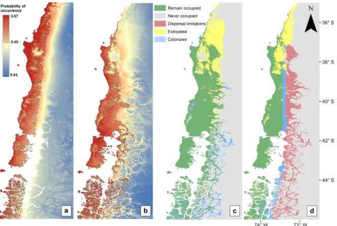
FIG. 2. (a) Maps showing predicted suitable climates for baseline (1965–1969) and (b) predictions for current climatic
and non-suitable habitats forR. darwinii(Appendix S7). Thereby, SDMs had to extrapolate into 2010 climatic conditions unrepresented in the calibration data set to be projected. The climatic novelties reported by the ExDet tool only occurred in the range of univariate vari-ation (i.e., exceeding the range of values of at least one climatic variable that occurred under the initial climatic conditions), with novel combinations between covariates not being observed. We found that no-analogue climate samples showed significantly lower performance (all Mann-WhitneyUfrom the three dispersal scenarios and two performance indexes<63, allP<0.05) and sensitiv-ity values (all Mann-Whitney test U <29, and P<0.001) than analogue samples, but no significant differences in model specificity were observed (all Mann-WhitneyU >74, andP>0.1), independently of the SDM framework (Fig. 5; for detailed U statistics and P values of analogue vs. no-analogue areas, see Appendix S6 in the Supporting Information).
DISCUSSION
Predicting species range shifts under global climate change is a major challenge for conservation biogeogra-phy (Araujo et al. 2005, Botkin 2007, Carvalho et al. 2011). However, the most commonly used approach to forecast range shifts, the habitat suitability models (or ecological niche models), have shortcomings that could limit their predictive accuracy over time (Elith and Leathwick 2009, Franklin 2013). Two key obstacles to predicting range shifts reliably under global change sce-narios are (1) lack of incorporation of dispersal pro-cesses (Miller and Holloway 2015) and (2) the environmental extrapolation of these models (Fitz-patrick and Hargrove 2009). We demonstrated the con-sequences of these shortcomings on predictability in time of SDMs using historical data contrasted with cur-rent presence–absence data.
Our results offer new insights to predict range shifts reliably. They support with empirical and time-indepen-dent results the recognized idea that incorporating dispersal processes would significantly improve the tem-poral predictability of SDMs (e.g., Pitelka 1997, Midg-ley et al. 2006, Schurr 2012, Eskildsen et al. 2013, Miller and Holloway 2015). This might help to reduce one of the most common sources of uncertainty of SDM pre-dictions, the difference between full and no dispersal sce-narios (Thuiller et al. 2006). Our results showed that model extrapolations could lead not only to higher uncertainties, but also to lower predictive accuracy over time. This is especially relevant as the rise of no-analo-gue climates is expected to be inevitable, and therefore reporting the geographic distribution of model extrapo-lation is key to informing conservation decisions better. Our results also support previous reports that model evaluation with non-temporal-independent data (i.e., data-splitting of the calibration data set) provides overly optimistic assessments of predictive accuracy over time; the time-independent data set is the most robust way to assess model accuracy over time (Araujo et al. 2005, Eskildsen et al. 2013).
While SDM forecasts usually show good predictability over time (i.e., AUC > 0.8; Kharouba et al. 2009, Dobrowski et al. 2011), the ability to predict changes in occupancy status due to climate change using SDMs that do not incorporate dispersal processes is at best weak (Rapacciuolo et al. 2012, Eskildsen et al. 2013). Two key processes that could limit the accuracy of SDMs in range shift predictions are the persistence of populations in habitats initially suitable and occupied, but that have become unsuitable; and the dispersal capacity to colonize new suitable habitats (i.e., to track climate change; Thuiller 2008, P€oyry et al. 2009, Devic-tor 2012, Lenoir and Svenning 2015), especially when the suitable habitat has been modified by human activi-ties, reducing landscape connectivity and limiting disper-sal processes (Vasudev et al. 2015). Incorporating dispersal processes not only has consequences for
FIG. 4. Boxplot (median, 25th, and 75th percentiles) of
reducing the uncertainty of projected range shifts needed in conservation planning (Carvalho et al. 2011, Aben et al. 2016), but also for extinction risk assessments. Usually, SDM projections using full dispersal assump-tions overestimate the geographical range area because these models are not able to distinguish an accessible habitat from that one that is inaccessible (Miller and Holloway 2015, Zurell 2016), and therefore might lead to incorrect estimations of extinction risk (Hamann and Aitken 2013). Moreover, the relationship between pro-jected suitable habitat (accessible and inaccessible) and extinction risk is often weak (Fordham 2012), and this apparent weakness could be explained by differences between incorporating or not the dispersal capacity of species when assessing the risk of extinction due to cli-mate change through SDMs. For R. darwinii, simple SDM forecasts predicted an increase in potential climati-cally suitable area. However, dispersal-constrained SDMs predicted decreases in the range area for 14 out of 15 replicates, highlighting that dispersal capacity plays an important role in accurate assessment of extinc-tion risk (Fig. 3). Even more, the results presented here could be considered as conservative because they do not incorporate land use change and its interactions with
climate change (Sohl 2014). If we had included land use change, the results could have shown even greater losses due to the dynamics of forests replacement experienced over the last 40 yr in central and southern Chile (Echeverrıa et al. 2006, Miranda et al. 2016).
Improvement in temporal predictability when dispersal constraints are included in SDMs is clearly explained by the desirable increase in model sensitivity (i.e., a decrease in false presence predictions). Model sensitivity has been suggested as more critical to model reliability to support conservation decisions than model specificity (Jim enez-Valverde et al. 2011). This is important in conservation management because the former allows more accurate reports of where the species is expected to spread and where the species should not colonize due to dispersal limitations, even though the model predicts suitable cli-mates. The increase in model sensitivity for R. darwinii using dispersal-constrained SDMs with respect to projec-tions from simple SDMs is consistent with large areas of habitat that have become suitable, but whichR. darwinii cannot reach due to dispersal limitations (e.g., high-lati-tude islands in Patagonian fjords and high altihigh-lati-tudes in the Andes; Fig. 2d). However, we did not observe improve-ments in SDM specificity (i.e., no decrease in false
FIG. 5. Boxplot (median, 25th, and 75th percentiles) of different measures of accuracy of species distribution models
absence predictions) when dispersal capacity was incor-porated. This could be interpreted as a limitation in the ability of SDMs to predict species distributional responses to climate change at the trailing edge of a spe-cies’range shift, which is not explained by dispersal con-straints. Two alternative explanations compete for false absence predictions. First, SDM projections are probably pessimistic in predicting habitat loss at the trailing edge, because SDMs are based on the realized climatic niche, which can be much narrower than the fundamental niche (Jackson and Overpeck 2000). This is also consistent with non-climatic range limitations, which have been proposed as likely the norm rather than the exception (Early and Sax 2014). Second, another overly pessimistic issue of SDM projections in the face of climate change is the assumption that populations under unsuitable conditions are committed to local extinction (e.g., Thomas et al. 2004). Therefore, these models rarely incorporate persis-tence of populations when the climate of a given area became unsuitable, which could explain at least part of false absence predictions (but see Dullinger 2012). This highlights the need for incorporating not only dispersal processes in dynamic SDMs, but also population persis-tence under unsuitable conditions (Schurr et al. 2007, Thuiller 2008), disentangling the effects of misrepresented niche and persistence in unsuitable habitats on the tempo-ral predictability of SDMs. An example of incorporating both processes is presented in Early and Sax (2011), who demonstrated that population persistence could be criti-cal to predict species range shifts. Moreover, Garc ıa-Valdes et al. (2015) showed that dispersal capacity was the best single predictor not only for colonization but also for extinction rates (along with climate) for most of the 23 species throughout mainland Spain. However, to our understanding, the consequences of incorporating popu-lation persistence in temporal predictability of SDMs have not been demonstrated so far (e.g., through time-independent validation of predictions). If persistence has an effect on the predictability of SDMs over time, its effects should be greater in long-lived species because of a greater temporal lag for local extinctions (climatic extinc-tion debts; Devictor 2012), assuming that it is somewhat unlikely that these populations could evolve to adapt to new conditions. Although most amphibians are expected to live for only few years, R. darwinii appears to live longer. Field studies have recorded adults a minimum of 8 yr old (C. Soto-Azat,personal communication), while in captivity, individuals have survived up to 15 yr (Busse 2002); this is a reason why the persistence of populations under unsuitable conditions should be considered in future forecasts of range dynamics for this species.
Current climate conditions are changing, with some climates disappearing and new ones emerging. However, reports of no-analogue climates to take account of pre-diction uncertainty are still an uncommon practice in species distribution forecasts (Elith and Leathwick 2009). Instead studies typically extrapolate models into no-analogue conditions and assume such extrapolations
are valid (Fitzpatrick and Hargrove 2009). Our results suggest that, similarly to spatial extrapolation (Heikki-nen et al. 2012), a good capability of SDMs to predict species distributions under training conditions does not guarantee equally good performance when these are transferred in time. In spite of this, environmental extrapolation seems to be a situation that often cannot be avoided when correlative SDMs are being transferred in space or time. For this reason, our findings demon-strate the importance of environmental extrapolation for temporal transference of SDMs, and is consistent with the recommendations of reporting the degree of environ-mental extrapolation both for temporal and spatial transference of SDMs (e.g., Elith et al. 2010, Zurell et al. 2012, Mesgaran et al. 2014) to prevent erroneous or imprecise predictions, or at least communicate where model predictions are reliable and where they are not. Bayesian Hierarchical models (e.g., Dynamic Range Models; Pagel and Schurr 2009) have been shown to pro-duce reliable predictions in time (using simulated data; Schurr 2012), with several advantages including the inference of spatiotemporal range dynamics in equilib-rium and non-equilibequilib-rium conditions, and the capacity of reporting the within-model uncertainty of the predic-tions. These advantages could be especially relevant in predicting range dynamics when models are transferred in time or space and extrapolated to novel environmen-tal conditions (Schurr 2012).
Significant improvements in temporal model pre-dictability can be obtained when realistic dispersal con-straints are included in dynamic SDMs, reducing the uncertainty of the over-simplistic approach of no or full dispersal scenarios. This may be more important for dis-persal-limited species, which have shown lower temporal predictability compared to species with high mobility. However, the predictive performance of SDMs signifi-cantly decreases in no-analogue climate areas, and as the rise of climatic novelty is inevitable, reporting the geo-graphic distribution of model extrapolation is key to bet-ter informed conservation decisions. Studies performing time-independent evaluations of SDM projections over time are needed, since this is a more robust way to assess the predictive accuracy of SDMs in a context of environ-mental change. Furthermore, the development of novel mechanistic models should include, in addition to dis-persal processes, population persistence in unsuitable habitats, thus accounting for local extinction debts or the ability of species to adapt, and thereby reducing false absences in model predictions.
ACKNOWLEDGMENTS
FONDECYT Iniciacion No 11140357, FONDECYT Ini-
LITERATURECITED
Aben, J., G. Bocedi, S. C. Palmer, P. Pellikka, D. Strubbe, C. Hallmann, J. M. J. Travis, L. Lens, and E. Matthysen. 2016. The importance of realistic dispersal models in plan-ning for conservation: application of a novel modelling plat-form to evaluate management scenarios in an Afrotropical biodiversity hotspot. Journal of Applied Ecology. https://doi. org/10.1111/1365-2664.12643
Allouche, O., A. Tsoar, and R. Kadmon. 2006. Assessing the accuracy of species distribution models: prevalence, kappa and the true skill statistic (TSS). Journal of Applied Ecology 43:1223–1232.
Araujo, M. B., R. G. Pearson, W. Thuiller, and M. Erhard. 2005. Validation of species-climate impact models under cli-mate change. Global Change Biology 11:1504–1513. Araujo, M. B., and C. Rahbek. 2006. How does climate change
affect biodiversity? Science 313:1396.
Barve, N., V. Barve, A. Jimenez-Valverde, A. Lira-Noriega, S. P. Maher, T. A. Peterson, J. Soberon, and F. Villalobos. 2011. The crucial role of the accessible area in ecological niche modeling and species distribution modeling. Ecological Modeling 222:1810–1819.
Bateman, B. L., H. T. Murphy, A. E. Reside, K. Mokany, and J. VanDerWal. 2013. Appropriateness of full-, partial-and no-dispersal scenarios in climate change impact modelling. Diversity and Distributions 19:1224–1234.
Botkin, D. B., et al. 2007. Forecasting the effects of global warming on biodiversity. BioScience 57:227–236.
Bourke, J. 2010.Rhinoderma darwiniicaptive rearing facility in Chile. Froglog 94:2–6.
Brown, J. H., D. W. Mehlman, and G. C. Stevens. 1995. Spatial variation in abundance. Ecology 76:2028–2043.
Brun, P., T. Kiørboe, P. Licandro, and M. R. Payne. 2016. The predictive skill of species distribution models for plankton in a changing climate. Global Change Biology. https://doi.org/ 10.1111/gcb.13274
Busse, K. 2002. Fortpflanzungsbiologie vonRhinoderma dar-winii (Anura: Rhinodermatidae) und die stammes-geschichtliche und funktionelle Verkettung der einzelnen Verhaltensabl€aufe. Bonner Zoologische Beitr€age 51:3–34. Carvalho, S. B., J. C. Brito, E. G. Crespo, M. E. Watts, and H.
P. Possingham. 2011. Conservation planning under climate change: toward accounting for uncertainty in predicted spe-cies distributions to increase confidence in conservation investments in space and time. Biological Conservation 144:2020–2030.
Climatic Research Unit Time-Series (CRU-TS). 2012. Historic climate database for GIS v3.10.01. http://www.cgiar-csi.org/ data/uea-cru-ts-v3-10-01-historic-climate-database
Crump, M. L. 2002. Natural history of Darwin’s frog, Rhino-derma darwinii. Herpetological Natural History 9:21–30. Davis, A. J., L. S. Jenkinson, J. H. Lawton, S. Shorrocks, and
S. Wood. 1998. Making mistakes when predicting shifts in species range in response to global warming. Nature 391:783– 786.
Devictor, V., et al. 2012. Differences in the climatic debts of birds and butterflies at a continental scale. Nature Climate Change 2:121–124.
Dobrowski, S. Z., J. H. Thorne, J. A. Greenberg, H. D. Safford, and A. R. Mynsberge. 2011. Modeling plant ranges over 75 years of climate change in California, USA: temporal transferability and species traits. Ecological Monographs 81:241–257.
Dormann, C. F. 2007. Promising the future? Global change pro-jections of species distributions. Basic and Applied Ecology 8:387–397.
Dormann, C. F., et al. 2012. Correlation and process in species distribution models: bridging a dichotomy. Journal of Biogeography 39:2119–2131.
Dullinger, S., et al. 2012. Extinction debt of high-mountain plants under twenty-first-century climate change. Nature Climate Change 2:619–622.
Early, R., and D. F. Sax. 2011. Analysis of climate paths reveals potential limitations on species range shifts. Ecology Letters 14:1125–1133.
Early, R., and D. F. Sax. 2014. Climatic niche shifts between species’native and naturalized ranges raise concern for eco-logical forecasts during invasions and climate change. Global Ecology and Biogeography 23:1356–1365.
Echeverrıa, C., D. Coomes, J. Salas, J. M. Rey-Benayas, A. Lara, and A. Newton. 2006. Rapid deforestation and frag-mentation of Chilean temperate forests. Biological Conserva-tion 130:481–494.
Elith, J., M. Kearney, and S. Phillips. 2010. The art of modelling range-shifting species. Methods in Ecology and Evolution 1:330–342.
Elith, J., and J. R. Leathwick. 2009. Species distribution models: ecological explanation and prediction across space and time. Annual Review of Ecology, Evolution, and Systematics 40: 677–697.
Engler, R., and A. Guisan. 2009. MigClim: predicting plant dis-tribution and dispersal in a changing climate. Diversity and Distributions 15:590–601.
Engler, R., W. Hordijk, and A. Guisan. 2012. The MIGCLIM R package-seamless integration of dispersal constraints into projections of species distribution models. Ecography 35:872– 878.
Eskildsen, A., P. C. le Roux, R. K. Heikkinen, T. T. Høye, W. D. Kissling, J. P€oyry, M. S. Wisz, and M. Luoto. 2013. Testing species distribution models across space and time: high lati-tude butterflies and recent warming. Global Ecology and Bio-geography 22:1293–1303.
Estrada, A., C. Meireles, I. Morales-Castilla, P. Poschlod, D. Vieites, M. B. Araujo, and R. Early. 2015. Species’ intrin-sic traits inform their range limitations and vulnerability under environmental change. Global Ecology and Biogeogra-phy 24:849–858.
Evans, M., C. Merow, S. Record, S. M. McMahon, and B. J. Enquist. 2016. Towards process-based range modeling of many species. Trends in Ecology & Evolution 31:860–871. FAO. 2001. FAOCLIM 2.0 A world-wide agroclimatic database.
Food and Agriculture Organization of the United Nations: Rome, Italy.
Fielding, A. H., and J. F. Bell. 1997. A review of methods for the assessment of prediction errors in conservation presence-absence models. Environmental Conservation 24:38–49. Fitzpatrick, M. C., and W. W. Hargrove. 2009. The projection
of species distribution models and the problem of non-analog climate. Biodiversity and Conservation 18:2255–2261. Fordham, D. A., et al. 2012. Plant extinction risk under climate
change: Are forecast range shifts alone a good indicator of species vulnerability to global warming? Global Change Biol-ogy 18:1357–1371.
Franklin, J. 2010. Moving beyond static species distribution models in support of conservation biogeography. Diversity and Distributions 16:321–330.
Franklin, J. 2013. Species distribution models in conservation biogeography: developments and challenges. Diversity and Distributions 19:1217–1223.
Guillera-Arroita, G., J. J. Lahoz-Monfort, J. Elith, A. Gordon, H. Kujala, P. E. Lentini, M. A. McCarthy, R. Tingley, and B. A. Wintle. 2015. Is my species distribution model fit for purpose? Matching data and models to applications. Global Ecology and Biogeography 24:276–292.
Guisan, A., and N. E. Zimmermann. 2000. Predictive habitat distribution models in ecology. Ecological Modelling 135:147–186.
Guisan, A., et al. 2013. Predicting species distributions for con-servation decisions. Ecology Letters 16:1424–1435.
Hamann, A., and S. N. Aitken. 2013. Conservation planning under climate change: accounting for adaptive potential and migration capacity in species distribution models. Diversity and Distributions 19:268–280.
Heikkinen, R. K., M. Marmion, and M. Luoto. 2012. Does the interpolation accuracy of species distribution models come at the expense of transferability? Ecography 35:276–288. Hijmans, R. J., S. Cameron, J. L. Parra, P. G. Jones, and A.
Jar-vis. 2005. Very high resolu-tion interpolated climate surfaces for global land areas. International Journal of Climatology 25:1965–1978.
Hijmans, R. J., S. Phillips, J. Leathwick, and J. Elith. 2014. Package dismo. http://cran.r-project.org/web/packages/dismo/ index.htm
Hutchinson, M. F., and T. B. Xu. 2013. ANUSPLIN version 4.4 user guide. Australian National University, Centre for Resource and Environmental Studies, Canberra, Australian Capital Territory, Australia.
Jackson, S. T., and J. T. Overpeck. 2000. Responses of plant populations and communities to environmental changes of the late quaternary. Paleobiology 26:194–220.
Jacques-Coper, M., and R. D. Garreaud. 2015. Characteriza-tion of the 1970s climate shift in South America. Interna-tional Journal of Climatology 35:2164–2179.
Jimenez-Valverde, A., and J. M. Lobo. 2007. Threshold criteria for conversion of probability of species presence to either-or presence-absence. Acta Oecologica 31:361–369.
Jimenez-Valverde, A., A. T. Peterson, J. Soberon, J. M. Over-ton, P. Aragon, and J. M. Lobo. 2011. Use of niche models in invasive species risk assessments. Biological Invasions 13: 2785–2797.
Kharouba, H. M., A. C. Algar, and J. T. Kerr. 2009. Historically calibrated predictions of butterfly species’ range shift using global change as a pseudo-experiment. Ecology 90:2213–2222. Kovar, R., M. Brabec, R. Vita, and R. Bocek. 2009. Spring migration distances of some Central European amphibian species. Amphibia-reptilia 30:367–378.
Krause, C. M., N. S. Cobb, and D. D. Pennington. 2015. Range shifts under future scenarios of climate change: dispersal abil-ity matters for Colorado plateau endemic plants. Natural Areas Journal 35:428–438.
Landis, J. R., and G. G. Koch. 1977. The measurement of obser-ver agreement for categorical data. Biometrics 33:159–174. Lenoir, J., and J. C. Svenning. 2015. Climate-related range
shifts-a global multidimensional synthesis and new research directions. Ecography 38:15–28.
Martınez, I., F. Gonzalez-Taboada, T. Wiegand, J. J. Camarero, and E. Gutierrez. 2012. Dispersal limitation and spatial scale affect model based projections ofPinus uncinataresponse to climate change in the Pyrenees. Global Change Biology 18: 1714–1724.
Merow, C., M. J. Smith, T. C. Edwards, A. Guisan, S. M. McMahon, S. Normand, W. Thuiller, R. O. Wuest, N. E.€ Zimmermann, and J. Elith. 2014. What do we gain from sim-plicity versus complexity in species distribution models? Ecography 37:1267–1281.
Mesgaran, M. B., R. D. Cousens, and B. L. Webber. 2014. Here be dragons: a tool for quantifying novelty due to covariate range and correlation change when projecting species distri-bution models. Diversity and Distridistri-butions 20:1147–1159. Midgley, G. F., G. O. Hughes, W. Thuiller, and A. G. Rebelo.
2006. Migration rate limitations on climate change-induced range shifts in Cape Proteaceae. Diversity and Distributions 12:555–562.
Miller, J. A., and P. Holloway. 2015. Incorporating movement in species distribution models. Progress in Physical Geography 0309133315580890.
Miranda, A., A. Altamirano, L. Cayuela, A. Lara, and M. Gonzalez. 2016. Native forest loss in the Chilean biodiversity hotspot: revealing the evidence. Regional Environmental Change. https://doi.org/10.1007/s10113-016-1010-7
Mittermeier, R. A., P. R. Gil, M. Hoffman, J. Pilgrim, T. Brooks, C. G. Mittermeier, J. Lamoreux, and G. A. B. Da Finseca. 2005. Hotspots revisited: Earth’s biologically richest and most endangered terrestrial ecoregions. University of Chicago Press, Conservation International, Chicago, Illinois, USA.
Moran-Ordonez, A., J. J. Lahoz-Monfort, J. Elith, and B. A.~ Wintle. 2017. Evaluating 318 continental-scale species distri-bution models over a 60-year prediction horizon: What fac-tors influence the reliability of predictions? Global Ecology and Biogeography. https://doi.org/10.1111/geb.12545 Pagel, J., and F. M. Schurr. 2009. Forecasting species ranges by
statistical estimation of ecological niches and spatial popula-tion dynamics. Global Ecology and Biogeography 21:293– 304.
Pearman, P. B., C. F. Randin, O. Broennimann, P. Vittoz, W. O. van der Knaap, R. Engler, G. Le Lay, N. E. Zimmermann, and A. Guisan. 2008. Prediction of plant species distributions across six millennia. Ecology Letters 11:357–369.
Phillips, S. J., R. P. Anderson, and R. E. Schapire. 2006. Maxi-mum entropy modeling of species geographic distributions. Ecological Modelling 190:231–259.
Pitelka, F. 1997. Plant migration and climate change. American Scientist 85:464–473.
Pliscoff, P., F. Luebert, H. H. Hilgerc, and A. Guisan. 2014. Effects of alternative sets of climatic predictors on species dis-tribution models and associated estimates of extinction risk: a test with plants in an arid environment. Ecological Modeling 288:166–177.
Poyry, J., M. Luoto, R. K. Heikkinen, M. Kuussaari, and€ K. Saarinen. 2009. Species traits explain recent range shifts of Finnish butterflies. Global Change Biology 15:732–743. R Core Team. 2014. R: a language and environment for
statisti-cal computing. Version 3.1.2, R Foundation for Statististatisti-cal Computing, Vienna, Austria.
Radeloff, V. C., et al. 2015. The rise of novelty in ecosystems. Ecological Applications 25:2051–2068.
Rapacciuolo, G., D. B. Roy, S. Gillings, R. Fox, K. Walker, and A. Purvis. 2012. Climatic associations of British species distri-butions show good transferability in time but low predictive accuracy for range change. PLoS ONE 7:e40212.
Rowland, E. L., J. E. Davison, and L. J. Graumlich. 2011. Approaches to evaluating climate change impacts on species: a guide to initiating the adaptation planning process. Envi-ronmental Management 47:322–337.
Schloss, C. A., T. A. Nu~nez, and J. J. Lawler. 2012. Dispersal will limit ability of mammals to track climate change in the Western Hemisphere. Proceedings of the National Academy of Sciences USA 109:8606–8611.
Schurr, F. M., G. F. Midgley, A. G. Rebelo, G. Reeves, P. Pos-chlod, and S. I. Higgins. 2007. Colonization and persistence ability explain the extent to which plant species fill their poten-tial range. Global Ecology and Biogeography 16:449–459. Schurr, F. M., et al. 2012. How to understand species’niches
and range dynamics: a demographic research agenda for bio-geography. Journal of Biogeography 39:2146–2162.
Sinclair, S. J., M. D. White, and G. R. Newell. 2010. How useful are species distribution models for managing biodiversity under future climates? Ecology and Society 1:5.
Singer, A., et al. 2016. Community dynamics under environ-mental change: How can next generation mechanistic models improve projections of species distributions?. Ecological Modelling 326:63–74.
Soberon, J., and A. T. Peterson. 2005. Interpretation of models of fundamental ecological niches and species’distributional areas. Biodiversity Informatics 2:1–10.
Sohl, T. L. 2014. The relative impacts of climate and land-use change on conterminous United States bird species from 2001 to 2075. PLoS ONE 9:e112251.
Soto-Azat, C., A. Valenzuela-Sanchez, B. T. Clarke, K. Busse, J. C. Ortiz, J. C. Ortiz, C. Barrientos, and A. A. Cunningham. 2013b. Is chytridiomycosis driving Darwin’s frogs to extinc-tion? PLoS ONE 8:e79862.
Soto-Azat, C., A. Valenzuela-Sanchez, B. Collen, J. M. Rowcliffe, A. Veloso, and A. A. Cunningham. 2013a. The population decline and extinction of Darwin’s frogs. PLoS ONE 8:e66957. Swets, J. A. 1988. Measuring the accuracy of diagnostic systems.
Science 240:1285–1293.
Thomas, C. D., et al. 2004. Extinction risk from climate change. Nature 427:145–148.
Thuiller, W., S. Lavorel, M. T. Sykes, and M. B. Araujo. 2006. Using niche-based modelling to assess the impact of climate change on tree functional diversity in Europe. Diversity and Distributions 12:49–60.
Thuiller, W., et al. 2008. Predicting global change impacts on plant species’distributions: future challenges. Perspectives in Plant Ecology Evolution and Systematics 9:137–152. Urban, M. C., et al. 2016. Improving the forecast for
biodiver-sity under climate change. Science 353:aad8466.
U.S. Geological Survey. 1996. GTOPO30. https://lta.cr.usgs.gov/ GTOPO30
Valenzuela-Sanchez, A., G. Harding, A. A. Cunningham, C. Chirgwin, and C. Soto-Azat. 2014. Home range and social analyses in a mouth brooding frog: testing the coexistence of paternal care and male territoriality. Journal of Zoology 294:215–223.
van Proosdij, A. S. J., M. S. M. Sosef, J. J. Wieringa, and N. Raes. 2016. Minimum required number of specimen records to develop accurate species distribution models. Ecography 39:542–552.
VanDerWal, J., L. Falconi, S. Januchowski, L. Shoo, and C. Storlie. 2012. SDM Tools: Species distribution modelling tools: Tools for processing data associated with species distribution modelling exercises. R package version 1.1-13. R Foundation for Statistical Computing, Vienna, Austria. http://CRAN.R-project.org/package=SDMTools
Vasudev, D., R. J. Fletcher Jr., V. R. Goswami, and M. Krish-nadas. 2015. From dispersal constraints to landscape connec-tivity: lessons from species distribution modeling. Ecography 38:001–012.
Watling, J. I., D. N. Bucklin, C. Speroterra, L. A. Brandt, F. J. Mazzotti, and S. S. Roma~nach. 2013. Validating predictions from climate envelope models. PLoS ONE 8:e63600. Zhu, K., C. W. Woodal, and J. S. Clarck. 2012. Failure to
migrate: lack of tree range expansion in response to climate change. Global Change Biology 18:1042–1052.
Zurell, D., J. Elith, and B. Schr€oder. 2012. Predicting to new environments: tools for visualizing model behaviour and impacts on mapped distributions. Diversity and Distributions 18:628–634.
Zurell, D., et al. 2016. Benchmarking novel approaches for modelling species range dynamics. Global Change Biology 22:2651–2664.
SUPPORTINGINFORMATION
Additional supporting information may be found online at: http://onlinelibrary.wiley.com/doi/10.1002/eap.1556/full
DATAAVAILABILITY