Do deep and comprehensive regional trade agreements help in reducing air pollution?

Texto completo

(1)Do Deep and Comprehensive Regional Trade Agreements help in Reducing Air Pollution? Inmaculada Martínez-Zarzoso*, University of Göttingen, Germany and University Jaume I, Spain Walid Oueslati**, Environment Directorate, Organisation for Economic Co-operation and Development, Paris, France. Published in: International Environmental Agreements, Accepted: 11 September 2018 https://doi.org/10.1007/s10784-018-9414-0. *. Address for correspondence: Department of Economics, Platz der Göttinger Sieben 3, 37073,. Göttingen (Germany). Email: [email protected]. Tel: +49551399770. **. Contact: 2, rue André Pascal - 75775 Paris Cedex 16,Email : [email protected] Tel : : +33 1 45 24 19 83. The opinions expressed in this paper are those of the authors and do not necessarily reflect the official views of the OECD or of the governments of its member countries. An earlier version of this paper appeared in the OECD Environment Working Paper Series (see Martinez-Zaroso, 2018).. 1.

(2) Do Deep and Comprehensive Regional Trade Agreements help in Reducing Air Pollution? Abstract. Environmental concerns are increasingly being incorporated into regional trade agreements (RTAs) to promote environmental quality and ultimately ensure compatibility between trade and environmental policies. This occurs in a context where air pollution and its effects on human health are of major concern. This paper investigates whether the proliferation and depth of environmental provisions (EPs) in RTAs are associated with lower concentration levels of particulate matter. We present an index of EPs in RTAs that measures the breadth and depth of the provisions and use it to estimate the effect of ratifying RTAs with different levels of EPs on changes in PM2.5 concentration levels in a panel of OECD countries over the 1999–2011 period. Using an instrumental variables strategy, we find that countries that have ratified RTAs with EPs show lower levels of PM2.5 concentrations when we control for scale, composition and technique effects and for national environmental regulations. Moreover, the PM2.5 concentration levels in the pairs of countries that belong to an RTA with EPs tend to converge for the country sample. The results also hold for a longer period of time (1990–2011) and a broader sample of 173 countries as well as for other pollutants, namely CO2 and NO2.. 1. Introduction The interactions between international trade and environmental quality have been widely recognized by scholars (Grossman and Krueger, 1991, Antweiller et al., 2001; Copeland and Taylor, 2003; López & Islam, 2008) and policy actors since the early 1990s. Trade and the environment was already identified as a relevant area in the 1992 Rio Earth Summit and also referred to in the Rio +20 agreement, in which more action was required to ensure that countries could pursue development policies with the necessary environmental protection to ensure a sustainable path of economic growth and social progress. The proliferation of regional trade agreements (RTAs), with more than 250 RTAs in effect in 2014, has been reinforced by slow progress in the multilateral negotiation arena, in both trade and environmental issues. Whereas recent RTAs usually refer to environmental quality, the World Trade Organization (WTO) has not always. 2.

(3) succeeded in integrating environmental issues in multilateral trade negotiations 1 , usually leaving these issues to environmental multilateral agreements (MEAs). Until now, MEAs have been focused on particular aspects related to global (e.g. Kyoto) and local climate change (Montreal Protocol), or conservation and biodiversity (CITES), among many other issues. However, their effectiveness is far from being generally recognized2. An increasing number of recently ratified RTAs have introduced environmental provisions (EPs) in the main text of the RTAs or in accompanying side agreements. These provisions aim to protect the environment and establish methods of collaborating on environmental issues (Morin and Jinnah, 2018; Yoo and Kim, 2015). The breadth and depth of the provisions vary widely by agreement. At a minimum, new RTAs tend to incorporate environmental issues in the preamble or in some articles dealing with investment issues or exceptions. Other RTAs include a chapter dedicated exclusively to environmental matters, whereas in. some cases,. environmental aspects are covered in a side agreement3. This paper advances the current status of the literature body on the nexus of international trade, trade agreements and the environment in two fronts. First, by categorizing RTAs according to the breadth and the depth of the EPs included in the RTAs or in the corresponding side agreements. This categorization is new 4 , theoretically reliable, replicable and justifiable and is used to further investigate the effects of trade agreements on environmental quality. Second, we focus on the effect of RTAs with EPs on PM2.55 population weighted concentrations and explore whether the inclusion of most comprehensive EPs in RTAs is associated with higher air quality in the ratifying countries, than in countries members of RTAs with less or no EPs. 1. There are, however, some exceptions. Some environmental issues are being discussed under Doha and the WTO Dispute Settlement Body (DSB) and the Appellate Body have ruled on several trade and environmental disputes since the WTO’s inception, creating an interesting precedent. 2 An excellent survey is presented in Mitchell, 2003. Although numerous studies have investigated the effectiveness of MEAs (e.g. Breitmeier, 2011; Helm . and Sprinz, 2000; Michell, 2006), no clear correlation has been established between the operation of the MEAs and the state of the environment. 3 Since 2007, the OECD has undertaken regular reviews of how environmental issues are treated in trade agreements (OECD, 2007) and providing and updating an inventory of RTAs with environmental provisions (EPs) (Gallagher and Serret, 2010 and 2011; George, 2013, 2014a and 2014b). The OECD reports refer to some ex-post assessments of environmental impacts (e.g. EU-Chile and the US for the RTAs recently signed (George, 2013)) and mention the difficulty in isolating the impact of the RTAs on environmental outcomes from other factors. 4 Morin and Jinnah (2018) assess climate-related provisions in preferential trade agreements (PTAs), but only along four dimensions. 5 PM2.5 refers to atmospheric particulate matters (PM) that have a diameter of less than 2.5 micrometer.. 3.

(4) Small airborne particles are among the most policy relevant pollutants. It is widely recognized that PM2.5 imposes a substantial burden on human health. Large cohortbased studies conducted by epidemiologists have provided evidence since at least 25 years that pollution by PM2.5 increases the rate of death, especially through increases in respiratory and heart diseases6. The existing literature investigating the effects of RTAs on emissions (Baghdadi, Martínez-Zarzoso and Zitouna, 2013; Ghosh and Yamarik, 2006; Zhou et al., 2017) only distinguishes between RTAs with or without EPs, but misses an important aspect of the distinction between agreements according to the level of EPs and their enforceability. We depart from it by including the breadth and depth of EPs in a model of the determinants of emissions, which is estimated using panel data and dynamic panel data techniques over the 1999-2011 period for OECD+BRIIC countries as well as for a global sample. This analysis is carried out within the context of the RTAs that went into effect over the study period. Our main results indicate that countries that have ratified RTAs with EPs show lower levels of PM2.5 concentrations when we control for scale, composition and technique effects. and for national. environmental regulations.. Moreover,. the. PM2.5. concentrations in the pairs of countries that belong to an RTA with EPs tend to converge for the country sample. The results also hold for a longer period of time (1990-2011) and a broader sample of 173 countries as well as for other pollutants. The rest of this paper is structured as follows. Section 2 reviews the literature on the impact of trade liberalization and RTAs on the environment. Section 3 presents the empirical framework and the modelling strategy while also outlining the methodology used to categorize EPs in RTAs and highlights the resulting categorisation. Section 4 presents and discusses the main empirical results. Finally, Section 5 draws some conclusions. 2. Literature Review 2.1 The Impact of Trade Liberalisation on the Environment The impact of trade liberalisation on the environment is a controversial topic. Increasing openness and trade generates a mixture of potential positive and negative. 6. Calculations based on existent studies suggest that ambient (outdoor) PM 2.5 caused about 3 million deaths worldwide in 2012 (Cohen et al., 2017; World Health Organization, 2016).. 4.

(5) effects on the environmental and natural resources of countries. For this reason, the interactions between trade and the environment have been widely investigated by economists in the last two decades. Early on, Grossman and Krueger (1991) focused on the environmental effects the North American Free Trade Agreement had when it went into effect and decomposed the environmental impact of trade liberalization into scale, technique and composition effects. This decomposition has been frequently used by the subsequent related literature (Antweiller et al., 2001; Stoessel, 2001; Cole and Elliot, 2003; Lopez & Islam, 2008), with some authors stating that when trade is liberalized all of these effects interact with each other (Copeland and Taylor, 2003; Managi et al., 2009). The scale effect indicates that an increase in global economic activity due to an increase in trade raises the total amount of pollution and, as a consequence, creates environmental damages. Thus, the scale effect is expected to have a negative impact on the environment. However, the evidence from the literature also reports that higher incomes have a positive effect on environmental quality (Grossman and Krueger, 1995; Copeland and Taylor, 2004). This suggests that when assessing the effects of growth and trade on the environment, we cannot automatically hold trade responsible for environmental damage (Copeland and Taylor, 2004). Since increasing incomes per capita are usually associated with a greater demand for environmental quality and in turn foster beneficial changes in environmental policy, the net impact on the environment remains unclear. This argument is linked to the so-called environmental Kuznets curve (EKC), which basically hypothesizes the existence of an inverted U-shaped relationship between environmental quality and per capita income. The EKC hypothesis states that environmental quality first decreases and then rises with increasing income per capita (Stern, 2004). In the last decades, numerous empirical studies have tested for the existence of an EKC (please see Dinda (2004), Carson (2010) and Stern (2004, 2014) for a summary of the empirical literature). The literature concludes that for pollutants with local and more short-term impacts, a significant EKC is more likely to hold than for global and long-term pollutants (Dinda, 2004; Carson, 2010). In line with Carson (2010), we argue that the focus should be shifted to the mechanisms and transmission channels that affect the income-environmental quality relationship. The technique effect is expected to have a positive impact on the environment. Researchers widely agree that trade is responsible for technology transfers and new 5.

(6) technology should benefit the environment if pollution per output is reduced. A reduction in the emission intensity results in a decline in pollution, holding constant the scale of the economy and the mix of goods produced. Recent studies suggest that this effect can, in some cases, prevail over the scale effect (Levinson, 2015). Finally, the impact of the composition effect of trade on the environment, namely the effect of a change in the basket of products exported after trade liberalization, is ambiguous. Trade based on comparative advantage results in countries specialising in the production and trade of those goods that a country is relatively efficient at producing. On the one hand, if a comparative advantage results from differences between countries in environmental regulations, countries could benefit economically from having lax regulations, resulting in possible environmental damage. The pollution haven hypothesis (PHH) predicts that trade liberalisation in goods leads to the relocation of pollution-intensive production from high-income countries with more stringent environmental regulations to low-income countries with lax environmental regulations. Developing countries could therefore enjoy a comparative advantage in pollution-intensive products and become pollution havens. On the other hand, if factor endowments are the main source of comparative advantage, the factor endowment hypothesis (FEH) claims that countries where capital is relatively abundant will export capital-intensive (dirty) goods. This stimulates production while increasing pollution in capital-rich countries. Countries where capital is scarce will see a fall in pollution given the contraction of the pollution generating industries. Thus, the economic theory predicts that the composition effect of liberalised trade on the environment depend on the distribution of comparative advantages across countries. Earlier studies using aggregate trade did not find much evidence of a pollution haven effect. Nevertheless, new studies using more disaggregate data, and accounting for endogeneity issues and spillovers, tend to find some support for it (Broner, Bustos and Carbalho, 2012; Millimet and Roy, 2015; Martínez-Zarzoso et al., 2016). In summary, the theoretical literature in economics identifies the existence of both positive and negative effects of the liberalisation of trade on the environment. The positive effects include increased growth and technology transfers accompanied by the distribution of environmentally safe, high-quality goods, services and technology. The negative effects stem from the relocation of pollution-intensive 6.

(7) economic activities in countries with lax environmental regulations that could potentially threaten the regenerative capabilities of ecosystems while increasing the danger of depleting natural resources. Most of the empirical literature has used changes in trade openness as a proxy for trade liberalisation (Antweiller et al., 2001; Cole and Elliot, 2003; Frankel and Rose, 2005; Managi et al., 2009). Roy (2017) is the only paper using intra-industry trade instead of overall trade. The main empirical findings point to net positive effects of overall trade on the environment and overall trade appears to be less proenvironment than intra-industry trade (Roy, 2017). The explanation for this net positive effect is that trade encourages innovation, speeds the absorption of new technologies and could also bring clean production techniques from more technologically advanced countries to the less advanced. Surprisingly, few studies have been devoted so far to regional trade agreements (RTAs), except in the case of NAFTA (Grossman and Krueger, 1991; Stern, 2007; Cherniwchan, 2017). Cherniwchan (2017) finds that, on average, about two-thirds of the reduction in PM10 emissions from the manufacturing sector in the United States can be attributed to NAFTA’s trade liberalization. To the best of our knowledge, only two more empirical studies have used RTAs instead of trade openness as a trade policy variable that could influence pollution levels or environmental outcomes in general (Ghosh and Yamarik, 2006; and Baghdadi et al., 2013). These two studies are described in detail in the next sub-section. However, it is worth noting that numerous studies in the field of international relations and political science have focused on the impact of RTAs on the environment in the Asian region (Vutha and Jalilian, 2008; and Yoo and Kim, 2015) and on the relation between the design of RTAs and environmental governance (e.g. Jinnah, 2011; Morin and Jinnah, 2018). Vutha and Jalilian (2008) focused on evaluating the possible impacts of trade on the environment, choosing ASEAN-China Free Trade Area (ACFTA) 7 as a case study to illustrate the relationship between RTAs and trade, and the implications of RTA-induced changes in trade flows on the environment. The authors state that they cannot offer any firm conclusion on the interaction between RTAs, trade and the environment for this specific case study 7. The ASEAN–China Free Trade Area (ACFTA), also known as China–ASEAN Free Trade Area is a free trade area among the ten member states of the Association of Southeast Asian Nations (ASEAN) and the People's Republic of China.. 7.

(8) given the complexity of the interlink and the limited data available after the ratification. Moreover, Yoo and Kim (2015) argue that recent RTAs have tended to enhance environmental cooperation among participating countries. Focusing in particular on the environmental policy changes in South Asian countries associated with the creation of its association agreements with ASEAN, the study concludes that each free trade agreement has incrementally developed environmental cooperation, especially when integrated into a vision for regional integration. Referring to the agreement between Peru and the US, Jinnah (2011) noticed that recently negotiated RTAs with EPs have the potential to enhance environmental regime effectiveness in ways that have been impossible under environmental treaties alone. Finally, Morin and Jinnah (2018) assess climate-related provisions in preferential trade agreements (PTAs) along four dimensions, namely innovation, legalization, replication and distribution. They find that some climate provisions are more specific and enforceable than some multilateral environmental agreements, such as the Kyoto protocol or the Paris Agreement. They assess the distribution of climate change provisions in PTAs by investigating whether they correlate with the level of emissions and find a negative correlation between levels of CO2 emissions and the average number of climate change provisions in PTAs. 2.2 The Impacts of RTAs on the Environment The first published study evaluating the quantitative impact of RTAs on the environment was Ghosh and Yamarik (2006). The authors proposed and estimated an empirical model where trade, growth and RTAs are linked and in which RTAs can have a direct and an indirect effect on the environment (through increasing trade and growth). Their empirical approach combines three well-known modelling strategies in the economics literature. First, the gravity model of trade, which has been considered the workhorse of empirical trade modelling since the early 1990s (Feenstra, 2016), is used to estimate the determinants of bilateral trade flows. Second, growth in GDP per capita is modelled following the growth-empirics literature that considers trade openness as one of the key factors in explaining economic growth (Frankel and Romer, 1990; Doyle and Martínez-Zarzoso, 2011). Finally, the above-mentioned literature linking trade with growth and environmental quality, based on the seminal work of Grossman and Krueger (1991) and Antweiller et al. (2001), is used to. 8.

(9) estimate the determinants of environmental degradation. As a proxy for degradation, three indicators of air quality (suspended particulate matter, sulfur dioxide and nitrogen dioxide) and four types of resource utilization (carbon dioxide per capita, percentage change in deforestation, energy depletion per capita and water pollution per capita) are considered. They apply ordinary least squares (OLS) in combination with instrumental variable estimation techniques (IV), the latter being used to control for the endogeneity of trade and income, to a sample of 151 countries in 1995 (using bilateral trade data for 1990). The main findings show that membership in RTAs reduces pollution by raising trade and income per capita, indicating that there is an indirect positive effect on environmental quality. In contrast, no evidence is found for the existence of a direct effect; for instance, they do not find any evidence that membership in RTAs itself affects environmental outcomes. There are three main limitations to Ghosh and Yamarik’s (2006) findings. First, it is based on data for a single year and therefore is unable to include the dynamics or to control for unobserved factors that are country-specific and time-invariant. Second, and perhaps the main shortcoming, is that the authors do not explain the mechanism through which the membership in RTAs could affect the environment. Finally, a third limitation is that there are important differences among RTAs in the way they take into account environmental issues. Whereas some RTAs include an extensive range of EPs (e.g. Canada-Panama), others are limited to confirming the general exceptions of GATT (art XIV and XIV) or exceptions for specific chapters (e.g. Australia-Malaysia). The two first issues are tackled in Baghdadi et al. (2013). Their approach refines and extends the modelling strategy applied in Ghosh and Yamarik (2006) by considering not only trade and GDP growth as endogenous variables, but also membership in RTAs. Moreover, the models are estimated for a panel-data set of 182 countries over the period from 1980 to 2008 and the endogeneity of the RTA variable is addressed by using matching and difference in differences (DID) techniques. The most remarkable departure from Ghosh and Yamarik (2006) is that Baghdadi et al. (2013) introduce the idea that if a direct positive effect of RTAs on the environment exists, it should only be found for those agreements that specifically include environmental provisions (EPs) in the main text of the trade agreement, or for those that are accompanied by side environmental agreements, as in the case of NAFTA 8. 8. Ghosh and Yamarik (2006) just mention that regional trade agreements address environmental issues and give the examples of NAFTA and the EU (page 20, second paragraph: “Whatever the route. 9.

(10) The direct effect is explained by the fact that EPs in RTAs will encourage members to apply and enforce more stringent environmental regulations and these should in turn enhance environmental quality. Hence, the link with regulations should induce an improvement in environmental outcomes independent of the trade-induced effect and even for similar levels of environmental regulations. In their paper, a distinction is made between RTAs membership in agreements with and without EPs. A limitation of this study is that EPs are very heterogeneous, with some RTAs including very detailed provisions and others only mentioning the environment in the investment chapter (e.g. OECD, 2007). Hence, modelling this using a dummy variable is over-simplistic. Moreover, a measure of national environmental regulations is missing in the analysis. The methodology in Baghdadi et al. (2013) consists of modelling per-capita CO2 emissions as a function of population, land area per capita, GDP per-capita, trade and RTAs. Since there could be reverse causality between the independent and the dependent variables, they assume that GDP per-capita and the trade variables are endogenously determined. The authors use instrumental variables (IV) techniques to estimate GDP per-capita (with a model borrowed from the growth-empirics literature) and trade (using a gravity model) and address RTA endogeneity due to self-selection into agreements using matching econometrics in combination with DID. To test whether countries’ CO2 emissions trajectories converge, a model for per-capita emissions is first estimated in relative terms using the log of carbon dioxide emissions per capita (log of CO2 emissions of country i relative to country j in period t, Emit/Emjt) as the dependent variable and expressing GDP per-capita, land area percapita and population also in relative terms. Next, the model is also estimated in absolute terms to examine the direct effect of RTAs on absolute pollution levels. In this case, the RTA variable is generated as a weighted average, using emissions in the partner countries as weights. The main results obtained from estimating the emissions model in relative terms provide evidence that RTAs with EPs statistically explain the convergence of CO2 levels across pairs of countries. Moreover, the agreements that specifically include provisions to ensure enforcement (NAFTA) are converging at a higher rate than others (EU), which leave compliance measures to the legal system. Conversely, RTAs without EPs do not affect relative pollution levels, indicating that controlling through which trading blocs impact the environment, regional trading arrangements are addressing environmental issues...”).. 10.

(11) for bilateral trade levels and overall openness, the trade policy variable (membership of RTAs) does not have a direct effect on emissions convergence for this type of agreements. The findings indicate that CO2 emissions are around 0.3 percent lower for countries that have RTAs with EPs, whereas the effect is not statistically significant for countries with RTAs without EPs. Hence, CO2 emissions converge to a lower level when both countries belong to the same RTA and the RTA includes EPs. With respect to the trade-environment link, the results do not show a significant effect of trade openness on the absolute levels of carbon dioxide emissions. More recently, in Zhou et al. (2017) an attempt is made to replicate Baghdadi et al. (2013) study using as dependent variable PM2.5 concentration levels instead of CO2. They presented estimates of the effect of countries participating in RTAs (with or without EPs) on emissions using a sample of 136 countries over a period of 10 years. They find that RTAs with environmental provision terms are likely to be associated with a lower level of PM2.5 concentrations and facilitate the convergence of PM2.5 concentrations between contracting countries. However, Zhou et al. (2017) included only countries with RTAs in most of their estimations and made only a distinction between RTAs with or without EPs without considering RTAs according to the level of EPs and their enforceability.. 3. Analytical Framework and Empirical Analysis In this section we present the analytical framework proposed to investigate the effect of EPs in RTAs on emissions, describe the target variables and construction of the environmental provision score and outline the modelling strategy. The main modelling strategy is partly based on Baghdadi et al. (2013) and consists of extending their approach to estimate the effects of trade and RTAs on a local pollutant using panel data and controlling for environmental regulations. The pollutant considered is particulate matter (PM2.5)9, which is used as the dependent variable in the empirical models. The corresponding explanatory variables and data sources are described in the data section below.. 3.1 Analytical Framework. 9. We use PM2.5 instead of SPM in this study. SPM refers to particles in the air of all sizes, whereas PM2.5, usually called fine particles, are not visible to the eye and are more harmful for health.. 11.

(12) Our analytical framework is based on the formal model-based definitions of the concepts of scale, composition and technique effects (Copeland and Taylor, 1994). It is also inspired by theories developed by Copeland and Taylor (2004) and Antweiller et al. (2001) relating trade and environmental regulations with environmental quality. Copeland and Taylor (2004) linked the environmental impact of trade liberalization to a country’s comparative advantage, to the choice of policy instruments and to the flexibility of the instruments. The authors noted that when analyzing the effects of trade and growth on environmental quality, one must account for endogenous policy responses. They found theoretical support for the hypothesis that more stringent regulations will have an effect on trade flows. However, trade theory suggests that many other factors, in addition to pollution regulation, will affect trade flows. Antweiller et al. (2001) presented an explicit pollution demand-and-supply model that divides trade’s impact on pollution concentrations into scale, technique and composition effects, with these effects varying across countries. The model allows income differences and factor abundance differences to jointly determine trade patterns. Their model predicts that the full effect of trade on pollution may be positive or negative, depending on the relative factor endowment of the country and on the strength of the technique and scale effects. Based on these theories, we take into account and introduce environmental regulations in an empirical framework that explains pollution concentrations with country characteristics, trade intensity and trade policy variables. We hypothesise that more stringent environmental regulations at the national level will reduce local air pollution after they are fully implemented and hence the effects will appear after some time. Moreover, for a given level of environmental regulations, participating in RTAs with EPs could also help reduce air pollution if the EPs provide enforcement mechanisms and encourage the member countries to effectively apply their national regulations. However, for RTAs without such provisions, countries may be less motivated to effectively enforce their regulations and there will be no additional effect on the environmental indicators coming from participation in RTAs without EPs. 3.2. Data sources and variables. 12.

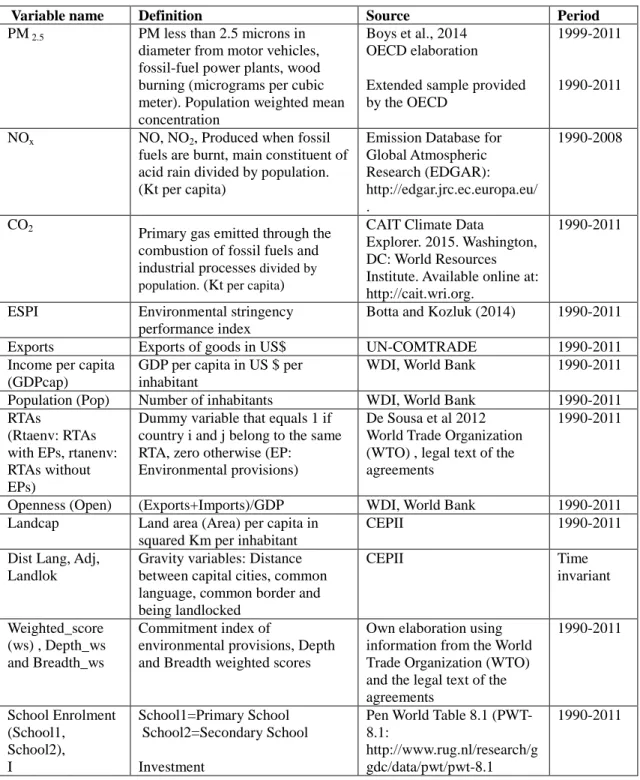
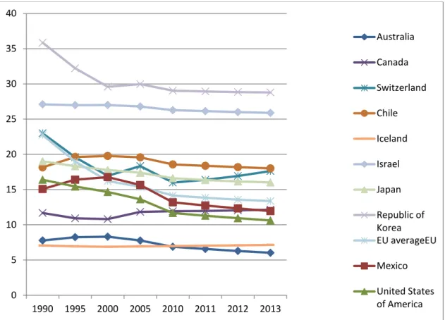
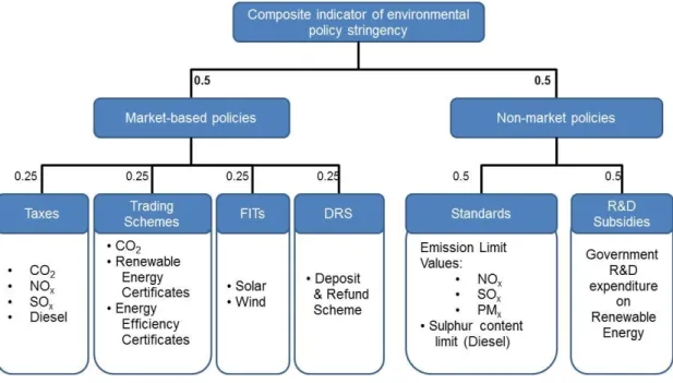
(13) Annual data for a cross-section of countries (mainly 23 OECD10+6 BRIICS11) over the period from 1999 to 2011 are used in the main empirical estimations. Moreover, we use an extended sample (173 countries) over the period 1990-2011 (data every 5 years for PM2.5).. Table 1. Description of Environmental Indicators, Data and Sources The main data for PM2.5 are from the OECD12. The variable used is the population weighted mean concentration of PM2.5. The data are available for a cross-section of 48 countries for the period from 1999 to 2011 (See Figure 1).. Figure 1. Population Weighted Concentrations of PM2.5 for Selected Countries Other variables used in the estimations of the empirical models are described in what follows. An environmental policy index, which measures the environmental policy stringency in OECD countries and has been constructed by the OECD13, is used as a proxy for policy interventions in the environmental area. The indicator is a composite country-specific measure of environmental policy stringency (ESPI). The current version of the indicator covers the above-mentioned 24 OECD countries plus the 6 BRIICS for the period 1990-2012. The indicator is based on scoring stringency of 15 policy instruments: 12 applying to the energy sector (though often to industry), 2 to transport and 1 in waste (Figure 2).. Figure 2. Economy-Wide ESPI Indicator Bilateral exports are from UN-COMTRADE and data for factors influencing bilateral trade, namely country and country pair characteristics are from CEPII. The ‘gravity’ variables used include distance between capital cities of the trading countries, dummy variables for a common language or past colony, exit to the sea, geographic size and a common border. 10. Australia, Austria, Belgium, Canada, Denmark, Finland, France, Germany, Greece, Hungary, Ireland, Italy, Japan, the Netherlands, Norway, Poland, Portugal, Slovakia, Spain, Sweden, Switzerland, the United Kingdom and United States. 11 Brazil, Russia, India, Indonesia, China and South Africa. 12 Data on PM2.5 are elaborated on by the OECD using datafrom the Atmospheric Composition Analysis Group (Boys et al., 2014). Available at: http://fizz.phys.dal.ca/~atmos/martin/?page_id=140. 13 See Botta and Kozluk (2014).. 13.

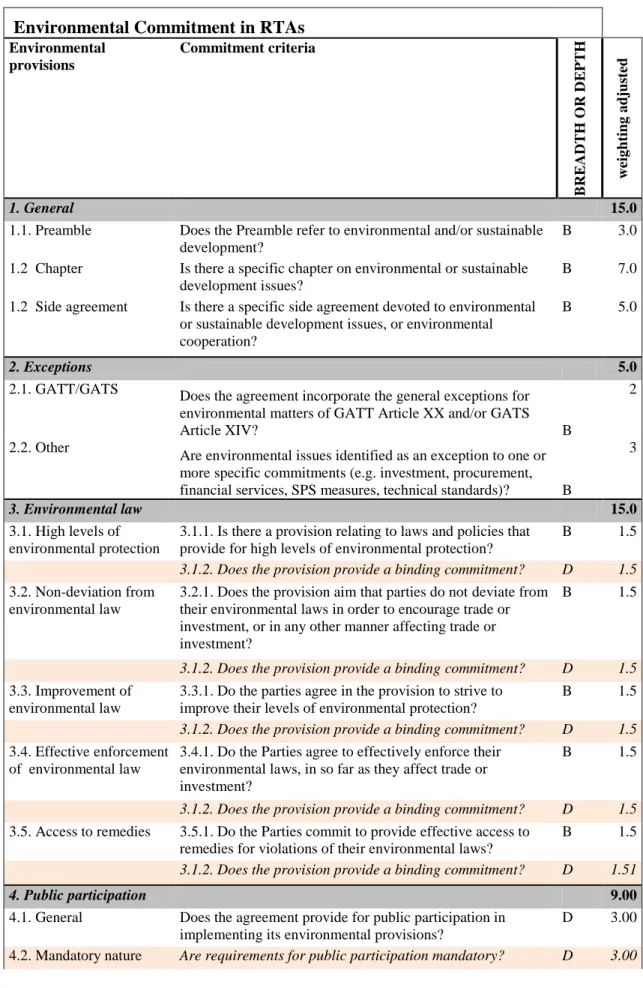
(14) Data for factors explaining income per capita in the growth regressions (population growth, school enrolment and the human development index) are from the WDI and the Pen World Table 8.114. Information concerning RTAs and the EPs included in each agreement has been collected from the World Trade Organization (WTO) and from the legal text of the agreements obtained from the corresponding government agencies of the signatory countries. 3.2.1 Categorisation of Environmental Provisions in RTAs On the basis of the key types of environmental provisions identified from the annual OECD updates on RTAs and the environment, a set of indicators on the degree of environmental commitment has been developed for an ex-post assessment of environmental provisions in RTAs. Different types of environmental provisions found in RTAs have been divided into nine categories for the purpose of this analysis: ‘General’, ‘Exceptions’, ‘Environmental Law’, ‘Public Participation’, ‘Dispute Settlement’, ‘Partnership and Co-operation’, ‘Specific Environmental Issues’, ‘Implementation Mechanism’ and ‘Multilateral Environmental Agreements’. Based on these nine key types of environmental provisions, three indicators on the degree of environmental commitment have been developed. The indicators are constructed using a number of questions relating to the content of the each RTA. Each question leads to a 0 or 1 answer (see Appendix 2). The questions are then weighted to give a total score for each RTA. Weights are adjusted to reflect the heterogeneity of different environmental provisions that may lead to differing impacts on the ultimate environmental outcome. In other words, the higher the expected impact of an environmental provision is, the higher the weight is given to that category. Weightings are adjusted so that there is not undue influence on a final score due to one particular over-weighted question or category. The total score for all questions across all categories is 100 in order to facilitate conversion of the index to a usable normalised variable. Questions are assigned either the breadth or depth label in case this will be a distinguishing characteristic in the model. In terms of breadth, the indicators aim to measure the degree of attention given to environmental issues in the agreement. In terms of depth, they aim to measure the extent to which the legal texts bind the parties to adhere to or implement their environmental provisions.. 14. PWT-8.1:http://www.rug.nl/research/ggdc/data/pwt/pwt-8.1.. 14.

(15) This weighting system aims to capture the relative importance of different types of provisions. Weights have been assigned based on a review of the OECD and other literature relating to the design, prevalence and implementation of environmental provisions (including George, 2014a; 2011; Gallagher and Serret, 2011; OECD, 2007)15. The ‘general’ category is assigned relatively high weighting because the inclusion of either a dedicated environmental chapter or an environmental side agreement (or both) is an important statement on the importance of the environment both legally and politically. The ‘environmental’ law category is also assigned a heavy weighting because these provisions are deemed to be an important means of leverage for RTA implementation to have an effect on environmental legislation in contracting parties. The Commitment of Multilateral Environmental Agreements (MEAs) is also regarded as a significant environmental provision because they can, in some instances, have precedence over trade regulation obligations where there are potential tensions between trade liberalization commitments and MEA trade-related measures (van Vooren et al., 2013). The obligations of MEAs shall prevail, in case of any inconsistency between the provisions and specific trade obligations set out in certain multilateral and bilateral environmental agreements.16 Considering that incoherence between the trade regulations and MEAs is an unresolved issue under the current WTO negotiations, this category is given relatively higher weight. Two categories of provision that relate to the implementation and operationalization of environmental provisions are given a moderate weighting: public participation and the implementation mechanism. These provisions have been highlighted in the OECD reviews as being important factors in achieving environmental commitments in RTAs. These two indicators relate to the actual operation of environmental commitments. Given that environmental outcomes would not arise from RTAs without the actual operation of the commitments, implementation mechanisms are considered important in this scoring method. The creation of a specific body to oversee implementation of the environmental provisions of a trade agreement is a factor in ensuring that the commitments made in the legal texts are implemented in practice. At the same time, the public participation is a fundamental component of the implementation. 15 16. Data on the breadth and depth indicators is available from the authors upon request. The provision on a legal precedence of MEAs roots from NAFTA in 1994, and presumably under the influence of NAFTA, most RTAs signed by Canada provide this provision.. 15.

(16) Transparency through the opportunity to participate in the decision-making process, the provision of effective access to judicial and administrative proceedings including redress and remedy, is important in ensuring that the environmental provisions in RTAs are actually implemented. In this regard, these two commitments are also given relatively higher weights. Although the category ‘specific environmental issues’ carries an overall higher weight, the category contains a large number of subquestions, all of which do not apply to any one particular RTA. Therefore, it would be very unlikely for an individual RTA to score a disproportionately high score for this category. Moreover, in every category, higher weights were allocated to individual questions relating to provisions, which are either binding or enforceable. For this purpose, sub-questions relating to ‘enforceability’ or ‘bindingness’ of provisions were embedded. Through these provisions, higher scores could be given to RTAs that not only mention a topic, but also have a provision that is binding or enforceable. Enforceability and bindingness is determined by the language used in these provisions, based on the enforceability index developed in Kohl et al. (2016). E.g. “shall” and “commit to” constitute a binding commitment; “strive to”, “encourage” are not binding. In contrast, the breadth of criteria in ’Specific environmental issues’ is assigned lower rates as they are usually brief statements or aspirations. 3.3 Modelling Strategy: Environmental-Impact Model According to the underlying theories that relate trade with the environment (e.g. Antweiller et al., 2001; Copeland and Taylor, 2004), environmental damage depends on population, per-capita GDP, openness to trade and RTAs. These variables are assumed to control for scale, technique and composition effects 17 . Panel data techniques are used to control for the endogeneity of the target variables (RTA, score, breadth and depth) in the environmental-impact model, whereas using instrumental variables will enable us to address the endogeneity of the income and trade variables. We will proceed with the description of the core equations for environmental impact. The details of the first step procedures for the instrumental variables estimation are explained in Appendix 1.. 17. Our model considers the main factors affecting emissions in line with Frankel and Rose (2005) and Baghdadi et al. (2013). Moreover, as in Frankel and Rose (2005) and Ghosh and Yamarik (2006), a Kuznets-curve term, namely the square term of the log of income per capita, is added in Model 1.. 16.

(17) First, to examine the direct effect of RTAs on absolute environmental quality, we specify the estimated equation as:. (1). where Eit, the natural logarithms of population-weighted PM2.5 for country i at time t, is the dependent variable 18 . All of the independent variables are also in natural logarithms apart from the two RTA variables. Population (Popit) is a proxy for the scale effect, GDP per capita predicted from a growth equation (. ) and its. squared term serve to test the EKC hypothesis that predicts that environmental quality eventually increases with income, predicted openness (. ) serves as proxy for the. composition effect and could be positively or negatively affecting environmental quality, as discussed in the previous section. The proxy used for environmental policy is the environmental policy stringency index (ESPIit), which is assumed to have a positive impact on environmental quality (negative effect on emissions). Nrtaenvit=. denotes agreements with EPs and Nrtanenvit= denotes RTAs without EPs. Both variables are generated as a weighted. average of the variables rtaenvijt (that takes the value of one when countries i and j have an RTA with EPs enforced in year t, zero otherwise), and rtanenvijt (that takes the value of one when countries i and j have an RTA without EPs enforced in year t, zero otherwise). wjt denotes the weights given to the different RTAs, equal weights for all agreements are used as default19. Hence the variable Nrtaenvit (Nrtanenvit) is the sum of the number of trading partners (j) that each country (i) has belonging to RTAs with EPs (without EPs), in a given year t. Finally, δt indicates the inclusion of year dummy variables (time fixed effects), which also serve as a proxy for the technique 18. A small part of PM2.5 can be considered as transboundary air pollution. However, there is no data available allowing the distinction between what has been emitted in a country and what goes through the borders. 19 Alternatively, we used bilateral trade lagged two years as weights in equation (1), the results remained similar in direction and statistical significance. Equal weights are selected to facilitate the interpretation of the results.. 17.

(18) effect that is common to all countries20. Equation (1) will be estimated distinguishing between RTAs with EPs and RTAs without EPs. In this way, we are able to test the prediction that only RTAs with EPs as a policy variable should affect a given environmental indicator directly, whereas RTAs without EPs should only affect the environment through trade or income. Next, model (1) is modified to include the described environmental commitment index and the depth and the breadth of the environmental commitments of the RTAs with EPs. Hence, the two dimensions of the provisions, depth and breadth and the overall score (described in section 3.2.1), which is the sum of breath and depth, are used separately in equation (1) to acknowledge that each of them can have a different effect on the given environmental indicators, so three different equations will be estimated. The same IV strategies, as described above, are used to identify the income and trade effects on the environment. We also use a panel data strategy21 as a way to overcome endogeneity issues. Second, following Baghdadi et al. (2013) who also tested for the convergence of emissions, we estimate a log-linear equation in relative terms in which the dependent variable is the log of the level of a given environmental indicator in country i relative to country j in period t (. ln(Eit/Ejt)|. The estimated model is. given by:. (2). 20. We also experimented with specific time trends for different groups of countries and the results concerning our target variable remained unchanged. Results are available upon request. 21 In a panel data framework, the inclusion of country and time fixed effects as regressors, together with the policy variable that identifies the before and after policy intervention (in the case when an RTA has begun to be enforced), is equivalent to a difference in differences strategy. See for example Galiani et al. (2005).. 18.

(19) where Popit (Popjt) is the population in terms of the number of inhabitants in country i (j) in year t. Landcapit (Landcapjt) is land area in square kilometres per capita, ( (j) in year t.. ) is predicted GDP per capita at constant US dollars in country i (. ) refers to the openness ratio measured as predicted. export- and import-openness ratio in country i (j). ESPIit (ESPIjt) is the environmental policy stringency index in country i (j) at year t.. denotes predicted. bilateral trade between countries i and j in period t (see Appendix A1.2) and rtaenvijt and rtanenvijt are dummy variables that take the value of 1 when countries i and j have an RTA enforced in year t with and without EPs, respectively. The details of the estimation used to obtain. are outlined in the Appendix. (A.1.1). Similarly, predicted openness (both bilateral and multilateral) is obtained from the estimation of a gravity model of trade using a large dataset on pair-wise trade (see Appendix A.1.2). In particular, we use Badinger’s specification of the gravity model (Badinger, 2008). The exponent of the fitted values across bilateral trading partners is aggregated to obtain a prediction of total trade for a given country. , which is used as regressor in model (1). The endogeneity of the. RTA variable is solved by using panel data techniques as suggested by Baier and Bergstrand (2007). As a robustness check, we also estimate a long-run version of model (1) in which the estimation technique used is the dynamic Generalized Method of Moments (GMM) for panel data (Arellano and Bond, 1991; Blundell and Bond, 2000). A considerable strength of the GMM method is the potential for obtaining consistent parameter estimates in the presence of measurement errors and endogenous righthand-side variables. In practical terms, when using panel data, the unobserved country-specific component is eliminated by taking the first differences of the leftand right-hand-side variables and the endogeneity issue is solved by using the lagged values of the levels of the endogenous variables as instruments. The model is specified as: (3) The validity of specific instruments can be tested in the GMM framework by using the Hansen test of over-identifying restrictions. In the context of this research, we consider as endogenous variables, the lagged dependent variable (. 19. and the.

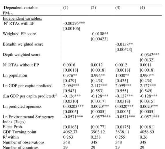
(20) variables related to an RTA with EP (rtaenv, score, breadth and depth) and the instruments used are the second and third lagged values in the levels of the respective variables. Next, we will examine whether the depth and the breadth of the RTA’s EPs contribute to convergence in environmental indicators between pairs of countries belonging to the same RTA. The estimated model is based on model (2), where RTAijt is replaced by. which measures the EP-commitment score and its two. dimensions, depth and breadth, of the agreement between countries i and j in year t (separate models are estimated for each variable: score, breadth and depth). The rest of the variables have been described below equation (2). Modifications of models (1) and (2) will be estimated using population-weighted PM2.5 concentrations as the dependent variable.. 4. Main Results This section presents the main results. Models (1) and (2) and their modified versions including the commitment index of EPs are estimated for PM2.5 (population weighted mean concentrations) and the main results are presented in Tables 2, 3 and 4. Yearly data for this pollutant are only available starting in 1999 and for a maximum of 48 countries. Alternatively, data is available at five-year intervals for a sample with 173 countries. The results we present in Table 2 are for a sample with 29 countries, for which the environmental policy proxy is available. The results are very similar to those obtained for the 48 sample presented in Appendix 4 (Table A.3.2). The within estimator with an autocorrelation term of order (1) is the preferred estimator22 and a non-linear effect for income is assumed (EKC hypothesis). Column (1) in Table 2 presents the estimates of the determinants of emissions and includes the variables Nrtaenv and Nrtanenv, the number of participants in RTA agreements signed by each country and year with and without EPs, respectively. The variable Nrtaenv shows a negative and significant coefficient (at the 5% level) indicating that for each additional bilateral RTA with EPs (in case of plurilateral agreements, for each additional country-member), the mean concentration of PM2.5 decrease by around 0.3 22. The model is estimated with the Stata command xtregar with fixed effects. Similar results were obtained with alternative specifications (e.g xtreg, fe and time dummies). The Hausman test suggested that the error term is correlated with time-invariant country heterogeneity, which suggests that only the within estimator is consistent. The model was also estimated using group specific time-dummies for OECD and non-OECD countries and no significant differences in the results were observed.. 20.

(21) percent, whereas Nrtanenv is not statistically significant. The negative and significant coefficient of only Nrtaenv indicates that RTAs with environmental provisions (EPs) have a direct negative effect on PM2.5 concentrations. The ESPI coefficient is also negative and statistically significant indicating that an increase in the index of 10 percent reduces concentrations by around 0.6 percent (this variable was entered with 3 lags and in general only the third lag is statistically significant, the coefficient shown in the table is the sum of the statically significant coefficients).. Table 2. Determinants of PM2.5 Emissions Concentrations The result for the income variables show evidence of a Kuznets-curve model with the squared coefficient of GDP per capita being statistically significant and showing the expected negative sign. It indicates that concentrations are negatively correlated with GDP per capita for income levels that surpass the turning point, which is shown at the bottom of the Table and is around 3.6-4 thousand USD. The sign and significance of the target variables Nrtaenv and ln ESPI are almost unchanged, in comparison to a model without the squared income term, except for the fact that ln ESPI shows a slightly lower coefficient, as expected. The predicted openness variable shows a positive coefficient that is always statistically significant at conventional levels, indicating that higher levels of trade do increase concentrations of PM2.5. However, the magnitude of the effect is close to zero and hence negligible in economic terms. For instance, an increase in trade of 100 percent is associated with an increase in PM2.5 concentrations of only 0.2 percent. In column (2) the target variable is the commitment index explained in the previous section. The result indicates that the score is negatively correlated with PM2.5 concentration levels and the same holds for the two dimensions of the index: breadth and depth (columns 3 and 4, respectively), with a higher magnitude observed for the coefficient for the depth dimension. An increase in 1 point in the breadth score decrease PM2.5 concentrations by around 1.6 percent, whereas the same increase in the depth score decrease PM2.5 concentrations by around 3.4 percent. Table 3 presents similar results to those shown in Table 2 using the extended sample of 173 countries23 for which the data are available every 5 years since 1990 23. The BRIICS countries used in this study hold some interesting policy insight into whether or not their membership in RTAs that have EPs leads to lower pollution. Since India and China are two. 21.

(22) until 2010 and then yearly until 2012. The results for the variable Nrtaenv (in column 1) show a negative and statistically significant coefficient (at the 5% level), which indicates that for each additional bilateral RTA with EPs, the mean concentration of PM2.5 decrease by around 0.5 percent (versus 0.3 percent in Table 2). On the other hand, Nrtanenv is also statistically significant (it was not in Table 2) but the effect is halved in comparison with the effect of Nrtaenv. The negative and statistically significant coefficients of both, RTAs with and without environmental provisions (EPs), could be due to the fact that in this case we are not able to control for domestic environmental regulations, since the ESPI indicator is only available for the small sample of countries used in the main results. It could be that some countries with RTAs without EPs also have more stringent regulations than others without RTAs.. Table 3. Determinants of PM2.5 Emissions Concentrations for 173 Countries Table 4 presents the results for convergence in emissions. The dependent variable is the ratio of PM2.5 concentrations per capita in natural logarithms. A negative sign in the target variables rtaenv (w_score, breath, depth) indicates that there is convergence in emissions between countries that participate in RTAs with EPs. The result in column (1) indicates that the rate of convergence is 9 percent for a pair of countries in RTAs with EPs and 12 percent in agreements without EPs. However, once the commitment index and its dimensions, instead of the simple dummy, are used as regressors (columns 2 to 4), the corresponding estimated coefficient for RTAs without EPs is not statistically significant, whereas the score, breadth and depth variables show a negative and statistically significant coefficient at the one percent level, indicating convergence in emissions in RTAs with more comprehensive EPs. The coefficient of bilateral exports (lexp_predict) is in most cases not statistically significant and the ESPI ratio present a negative coefficient indicating that convergence in environmental regulations is negatively correlated with convergence in emissions of PM2.5. countries with cities that have some of the worst PM2.5 emission concentrations in the world, their membership in RTAs (whether in breadth or depth), which may potentially lower air pollution, can provide some interesting policy insight. Of course, given that these are only 6 countries, data constraints prevent us from showing the empirical results for these 6 countries in a similar format as Tables 2 and 4. However our main results in our extended sample remain unchanged even after removing the 2 outlier countries of China and India. We thank an anonymous referee for this suggestion.. 22.

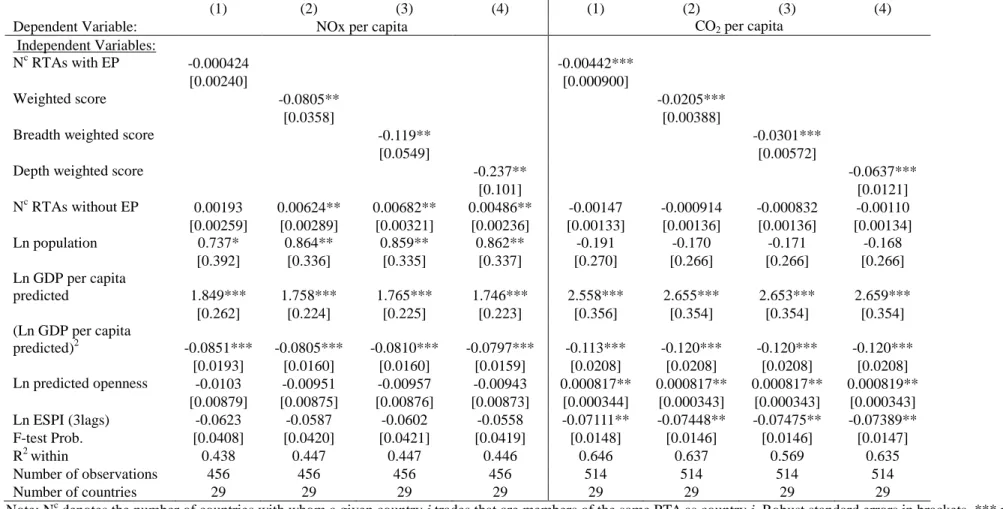
(23) Table 4. Determinants of Convergence in PM2.5 Emissions 4.3. Robustness As a robustness check we use another two pollutants, namely nitrogen oxide (NOx) and CO2 to obtain estimates for Model (1) using the same sample of countries as for PM2.5 in Table 2. The results are shown in Table A.3.1. The first part of the table shows the results for NOx. In this case, only the coefficient of the commitment index (w_score) and the breadth and depth components (depth) are statistically significant indicating that higher scores of the provisions are negatively correlated with emission of NOx; however, the mere membership criteria is not showing a statistically significant coefficient. Moreover, the proxy for environmental regulations shows a negative but non-significant coefficient, indicating that higher levels of regulatory stringency do not have a reducing effect on NOx emissions. As the environmental stringency index is a composite of market- and non-market-based policies, it could be that it does not capture the specific effect on single pollutants. For further research, it should be desirable to use instead of separate components in the index. The second part of Table A.3.1 shows the results for CO2. These results are more in line with those obtained for PM2.5. On the one hand, we observe negative and statistically significant coefficients for the target variables (RTA with EPs, score and its dimensions) and on the other hand, the stringency of environmental regulations also shows a negative and statistically significant effect on the levels of CO2 emissions. Given that CO2 is a global pollutant, this has important policy implications on further negotiations of RTAs. Model (1) has been also estimated for an extended sample of 48 countries with yearly data of population weighted PM2.5 emissions using a panel data model with country and time fixed effects and also using a dynamic panel data estimator, namely, difference GMM (dif-GMM, Arellano and Bond, 1991). The results are shown in Appendix 3 (Tables A.3.2 and A.3.3, respectively). In general, the results shown in Table A.3.2 for the 48-country sample confirm the results obtained for the smaller sample of 29 countries. The fact that the estimated. 23.

(24) effects are slightly different in magnitude is not only due to the addition of 19 countries but also because we are not able to include the ESPI among the regressors24. The results shown in Table A.3.3 using dif-GMM (with a lagged dependent variable and the model in first differences) confirm those obtained with the static panel data models indicating that both, membership in RTAs with EPs as well as an incremental inclusion of environmental issues in the text of the agreements, contribute to improving environmental quality. In general, the dif-GMM long-run estimates in Table A.3.3 show stronger effects than the estimates in the main text, which could be interpret as short-run effects. Finally, In order to check whether spatial dependence across countries affects the accuracy of our estimates, we have run the models allowing for standard errors that are heteroskedasticity consistent and robust to general forms of cross-sectional (spatial) and temporal dependence 25. The point estimates are very similar to those shown in the main results and in most cases the standard errors are smaller in magnitude, providing more accurate estimates. A more comprehensive modelling of the spatial dependence of the pollution observed is undoubtedly an interesting avenue of future research.. 5. Discussion and Conclusions The main results show that RTAs with EPs have a reducing effect on air pollution measured using PM2.5 emissions concentrations and also help emissions to converge among the participants in the RTAs. The empirical results indicate that a direct positive effect of RTAs on reducing air pollution exists, which is mainly present for those agreements that specifically include environmental provisions (EPs) in the main text of the trade agreement, or for those that are accompanied by side environmental agreements. The direct effect could be explained by the fact that the EPs in RTAs will encourage members to apply and enforce more stringent environmental regulations and these should in turn reduce environmental damage. Hence, the link with regulations induces a decrease in environmental degradation 24. To investigate the effect that excluding ESPI has on the results for the target variables, we estimated the model for the sample of 29 countries without ESPI. The estimated coefficients for rtaenv, w_score, breadth and depth are -0.0033, -0.0166, -0.0171 and -0.0362, respectively. Hence, these effects are shown as an upward bias in the coefficients of the variables (compare with -0.00295, -0.0108, -0.0158 and -0.0342 in Table 2). 25 We would like to thank one anonymous referee for raising this issue. The Stata command xtscc has been used, which is appropriate when the time dimension becomes large. The results are available upon request from the authors.. 24.

(25) independent of the trade-induced effect. This effect is also independent from the effect induced by other national environmental policies that are summarized in the environmental performance index, which is also used as an explanatory variable in the regressions. The results also indicate that the content of the EPs also matter for the environment. Indeed, the results show that higher levels of environmental regulations are also positively correlated with environmental quality. In particular, this is the case for PM2.5 emissions concentrations. The practice of including provisions that refer to the environment in trade agreements is a complementary way to address climate change, environmental degradation and related issues that should in any case be discussed at the international level in multilateral negotiations. In particular, joint international action is needed to place a cap on greenhouse gas (GHG) emissions and the recent outcome of the 2015 United Nations Climate Change Conference of Parties (COP21), held in Paris, is an excellent starting point. In fact, our results point towards a certain complementary relationship between domestic environmental policy and trade policy. This means that in addition to stringent environmental regulation, the use of environmental provision in trade agreements can improve environmental outcomes. Although these findings appear to have important implications for environmental provisions in ongoing negotiations of RTAs, we have to bear in mind that the analysis is not free from challenges and limitations. For instance, measuring the environmental end points in a given country is a difficult exercise. Air emissions of PM2.5 are known to be domestic pollutants and may not be a perfect proxy to represent environmental quality at the national level. Similarly, air emissions do not respect country borders, so measuring air emission concentrations within a small country, such as Panama, and relating it to Panama's number of trade agreements, may also be a challenge. Even with a focus on air emissions, PM2.5 data is only available for around 10 years and enables analysis for only 48 countries, whereas RTAs with environmental provisions cover a broader cross-section of countries for a period of more than two decades. Finally, the narrow definition of environmental provisions applied in this study may affect the results. A broader definition would classify the majority of RTAs as those with environmental provisions and may have different implications on the analysis. For this reason, we mainly rely on the results using the score rather than on those obtained using the number of RTAs. These findings should be validated in 25.

(26) future research, given the limitations on data availability in terms of coverage for the environmental quality indicators, countries, the time period and the different interpretations of environmental provisions in RTAs. Further analysis is also needed to shed light on the channels through which environmental provisions in RTAs may influence domestic policy processes and ultimately the environmental outcomes. The currently existing environmental policy stringency indicators are only available for a limited number of countries and do not capture the stringency of environmental policy in the developing countries that are sought to have improved their environmental policies in accordance with progressive environmental provisions in RTAs. Environmental policy indicators that cover both developed and developing countries would be required to further develop such analysis. In this sense, the current investigation could be extended using proxies for environmental regulations (treaties and laws) using a broad sample of countries.. References Antweiler W., Copeland, B. R. & Taylor, M. S. (2001). Is free trade good for the environment?. American Economic Review, 91(4), 877-908. Arellano, M. & Bond, S. (1991). Some Tests of Specification for Panel Data: Monte Carlo Evidence and Application to Employment Equations. Review of Economic Studies, 58, 227-297. Badinger, H., (2008). Trade policy and productivity. European Economic Review, 52, 867-891. Baghdadi, L., Martínez-Zarzoso, I. & Zitouna, H. (2013). Are RTA agreements with environmental provisions reducing emissions?, Journal of International Economics, 90(2), 378-390. Baier, S. L., & Bergstrand, J. H. (2007). Do free trade agreements actually increase members’ international trade?. Journal of International Economics, 71, 72-95. Botta, E. & Kozluk, T. (2014). Measuring environmental policy stringency in OECD countries - a composite index approach. OECD ECO Working Paper 1177, OECD Publishing. Blundell, R.W. & Bond, S.R. (1998). Initial Conditions and Moment Restrictions in Dynamic Panel Data Models. Journal of Econometrics, 87, 115-143.. 26.

(27) Broner, F., Bustos, P. & Carvalho, V. (2012). Sources of comparative advantage in polluting industries. NBER WP, No. w18337. Boys, B.L., Martin, R.V., van Donkelaar, A., MacDonell, R., Hsu, N.C., Cooper, M.J., Yantosca, R.M., Lu, Z., Streets, D.G., Zhang, Q. & Wang, S. (2014). Fifteenyear. global. time. series. of. satellite-derived. fine. particulate. matter.. Environmental Science & Technology, 48(19), 11109-11118. Breitmeier, H.; Underdal, A. & Young, O. R. (2011). The effectiveness of international environmental regimes comparing and contrasting findings from quantitative research. International Studies Review, 13, (4), 579-605. Carson, R. T. (2010). The environmental Kuznets curve: seeking empirical regularity and theoretical structure. Review of Environmental Economics and Policy, 4 (1), 3-23. Cherniwchan, J. (2017). Trade liberalization and the environment: Evidence from NAFTA and U.S. manufacturing. Journal of International Economics, 105, 130-149. Cohen, A.J., Brauer, M., Burnett, R., Anderson, H.R. et al. (2017). Estimates and 25year trends of the global burden of disease attributable to ambient air pollution: an analysis of data from the Global Burden of Diseases Study 2015. The Lancet, 389 (10082), 1907–1918. Cole, M.A. & Elliott, R.J. (2003). Determining the trade-environment composition effect: the role of capital, labor and environmental regulations. Journal of Environmental Economics and Management, 46(3), 363-83. Copeland, B.R. & Taylor, M.S. (1994). North-South trade and the environment. Quarterly Journal of Economics, 109(3), 755-787. Copeland, B.R. & Taylor, M.S. (2003). Trade and the environment: theory and evidence. Princeton, NJ: Princeton University Press. Copeland, B.R. & Taylor, M. S. (2004). Trade, growth, and the environment. Journal of Economic Literature, 42(1), 7-71. De Sousa, J. (2012). The currency union effect on trade is decreasing over time. Economics Letters, 117(3), 917-920. Dinda, S. (2004). Environmental Kuznets curve hypothesis: A survey. Ecological Economics, 49, 431-455. Doyle, E. & Martínez-Zarzoso, I. (2011). Productivity, trade and institutional quality: A panel analysis. Southern Economic Journal, 77 (3), 726-752. 27.

(28) Feenstra, R.C. (2016), Advanced international trade. Theory and Evidence, Princeton University Press. Frankel, J. & Romer, D. (1999). Does trade cause growth?. American Economic Review, 89(3), 379-399. Frankel J.A. & Rose, A.K. (2005). Is trade good or bad for the environment? Sorting out the causality. The Review of Economics and Statistics, 87, 85-91. Galiani, S., Gertler, P. & Schargrodsky, E. (2005). Water for life: The impact of the privatization of water services on child mortality. Journal of Political Economy, 113 (1), 83-120. Gallagher, P. & Serret, Y. (2010). Environment and regional trade agreements: developments in 2009. OECD Trade and Environment Working Papers, No. 2010/01, OECD Publishing, Paris. DOI: http://dx.doi.org/10.1787/5km7jf84x4vk-en. Gallagher, P. & Serret,Y. (2011). Implementing regional trade agreements with environmental provisions: A framework for evaluation. OECD Trade and Environment Working Papers, No. 2011/06, OECD Publishing, Paris. DOI: http://dx.doi.org/10.1787/5kg3n2crpxwk-en. George, C. (2013). Developments in regional trade agreements and the environment: 2012 Update. OECD Trade and Environment Working Papers, No. 2013/04, OECD Publishing. George, C. (2014a). Environment and regional trade agreements: emerging trends and policy drivers. OECD Trade and Environment Working Papers, No. 2014/02, OECD Publishing. George, C. (2014b). Developments in regional trade agreements and the environment: 2013 Update. OECD Trade and Environment Working Papers, No. 2014/01, OECD Publishing. Ghosh, S. & Yamarik, S. (2006). Do regional trading arrangements harm the environment? An analysis of 162 countries in 1990. Applied Econometrics and International Development, 6(2), 15-36. Grossman G.M. & Krueger, A.B. (1991). Environmental impacts of the North American free trade agreement. NBER working paper 3914. Grossman G.M. & Krueger, A.B. (1995). Economic growth and the environment. Quarterly Journal of Economics, 110(2), 353-377.. 28.

(29) Kohl, T., Brakman, S. & Garretsen, J. (2016). Do trade agreements stimulate international trade differently? Evidence from 296 trade agreements. World Economy, 39 (1), 97-131. Helm, C. & Sprinz, D. (2000). Measuring the Effectiveness of International Environmental Regimes. The Journal of Conflict Resolution, 44, (5), 630-652. Jinnah, S. (2011). Strategic linkages: the evolving role of trade agreements in global environmental governance. The Journal of Environment & Development, 20 (2), 191-215. Levinson, A. (2015). A direct estimate of the technique effect: Changes in the pollution intensity of US manufacturing, 1990-2008. Journal of the Association of environmental and Resource Economist, 2(1), 34-56. López, R. & Islam, A. (2008). Trade and the environment, The Princeton Encyclopedia of the World Economy. Princeton University Press, Princeton, New Jersey. Managi S., Hibiki, A. & Tsurumi, T. (2009). Does trade openness improve environmental quality?. Journal of Environmental Economics and Management, 58(3), 346-363. Martínez-Zarzoso, I., Vidovic, M. & Voicu, A. (2016). Are the Central East European Countries pollution havens?. The Journal of Environment and Development, 26, 25-50. Martínez-Zarzoso, I. (2018). Assessing the effectiveness of environmental provisions in regional trade agreements: An empirical analysis. OECD Trade and Environment Working Papers, 2018/02, OECD Publishing, Paris. http://dx.doi.org/10.1787/5ffc6 15c-en. Millimet, D.L. & Roy, J. (2016). Empirical test of the Pollution Haven hypothesis when environmental regulation is endogenous. Journal of Applied Econometrics, 31(4), 652-677. Mitchell, R.B. (2003). International environmental agreements: A survey of their features, formation and effects. Annual Review of Environment and Resources, 28, 429–61. Mitchell, R. B., (2006). Problem structure, institutional design, and the relative effectiveness of international environmental agreements. Global Environmental Politics, 6, (3), 72-89. OECD (2007). Environment and regional trade agreements, OECD Publishing, Paris. 29.

(30) Morin, J-F. & Jinnah, S. (2018). The untapped potential of preferential trade agreements for climate governance. Environmental Politics, 27(3), 541-565. OECD (2017). Green Growth Indicators 2017, OECD Publishing, Paris. DOI: http://dx.doi.org/10.1787/9789264268586-en. Roy, J. (2017). On the environmental consequences of intra-industry trade. Journal of Environmental Economics and Management, 83, 50-67. Stern, D. I. (2004). The rise and fall of the Environmental Kuznets Curve. World Development 32 (8), 1419-1439. Stern, D. I., (2007). The effect of NAFTA on energy and environmental efficiency in Mexico. The Policy Studies Journal, 35(2), 291-322. Stern, D.I. (2014). The Environmental Kuznets Curve: A primer. CCEP Working Paper 1404. Centre for Climate Economic & Policy, Australian National University. Stoessel, M. (2001). Trade liberalization and climate change. The Graduate Institute of International Studies, Geneva. Van Vooren, B., Blockmans, S. & Wouters, J. (eds.) (2013). The EU’s Role in Global Governance, Oxford: Oxford University Press. Vutha, H. & Jalilian, H. (2008). Environmental Impacts of the ASEAN-China Free Trade Agreement on the Greater Mekong Sub-Region. International Institute for Sustainable Development. http://www.iisd.org. World Health Organization (2016). Ambient air pollution: A global assessment of exposure and burden of disease. WHO Press, Geneva, Switzerland. Yoo, I. T. & Kim, I. (2015). Free trade agreements for the environment? Regional economic integration and environmental cooperation in East Asia. International Environmental Agreements: Politics, Law and Economics, 16 (5), 721–738. Zhou, L., Tian, X. and Zhou, Z. (2017). The effects of environmental provisions in RTAs on PM2.5 air pollution, Applied Economics 49 (7), 2630-2341.. 30.

(31) TABLES Table 1. Description of Variables, Data and Sources Variable name PM 2.5. NOx. CO2. ESPI Exports Income per capita (GDPcap) Population (Pop) RTAs (Rtaenv: RTAs with EPs, rtanenv: RTAs without EPs) Openness (Open) Landcap Dist Lang, Adj, Landlok. Weighted_score (ws) , Depth_ws and Breadth_ws. School Enrolment (School1, School2), I. Definition PM less than 2.5 microns in diameter from motor vehicles, fossil-fuel power plants, wood burning (micrograms per cubic meter). Population weighted mean concentration NO, NO2, Produced when fossil fuels are burnt, main constituent of acid rain divided by population. (Kt per capita) Primary gas emitted through the combustion of fossil fuels and industrial processes divided by population. (Kt per capita) Environmental stringency performance index Exports of goods in US$ GDP per capita in US $ per inhabitant Number of inhabitants Dummy variable that equals 1 if country i and j belong to the same RTA, zero otherwise (EP: Environmental provisions) (Exports+Imports)/GDP Land area (Area) per capita in squared Km per inhabitant Gravity variables: Distance between capital cities, common language, common border and being landlocked Commitment index of environmental provisions, Depth and Breadth weighted scores. School1=Primary School School2=Secondary School Investment. 31. Source Boys et al., 2014 OECD elaboration. Period 1999-2011. Extended sample provided by the OECD. 1990-2011. Emission Database for Global Atmospheric Research (EDGAR): http://edgar.jrc.ec.europa.eu/ . CAIT Climate Data Explorer. 2015. Washington, DC: World Resources Institute. Available online at: http://cait.wri.org. Botta and Kozluk (2014). 1990-2008. UN-COMTRADE WDI, World Bank. 1990-2011 1990-2011. WDI, World Bank De Sousa et al 2012 World Trade Organization (WTO) , legal text of the agreements. 1990-2011 1990-2011. WDI, World Bank CEPII. 1990-2011 1990-2011. CEPII. Time invariant. Own elaboration using information from the World Trade Organization (WTO) and the legal text of the agreements Pen World Table 8.1 (PWT8.1: http://www.rug.nl/research/g gdc/data/pwt/pwt-8.1. 1990-2011. 1990-2011. 1990-2011. 1990-2011.

(32) Table 2. Determinants of PM2.5 emissions concentrations in OECD and BRIIC countries. Dependent variable: PM2.5 Independent variables: Nc RTAs with EP. (1). (2). (3). -0.00295*** [0.00106]. Weighted EP score. -0.0108** [0.00423]. Breadth weighted score. -0.0158** [0.00623]. Depth weighted score Nc RTAs without EP Ln population Ln GDP per capita predicted (Ln GDP per capita predicted)2 Ln predicted openness Ln Environmental Stringency Index (3lags) F-test Prob. GDP Turning point R2 within Number of observations Number of countries. (4). 0.0016 [0.0018] 0.976** [0.429] 2.094*** [0.543] -0.126*** [0.0310] 0.00203*** [0.0005] -0.0571***. 0.0012 [0.0018] 0.996** [0.434] 2.117*** [0.553] -0.128*** [0.0317] 0.0020*** [0.0005] -0.0577***. 0.0012 [0.0018] 1.000** [0.435] 2.099*** [0.555] -0.127*** [0.0318] 0.0020*** [0.0005] -0.0571***. -0.0342*** [0.0132] 0.0011 [0.0018] 0.990** [0.434] 2.127*** [0.549] -0.128*** [0.0315] 0.0020*** [0.0005] -0.0571***. [0.0163] 4062.37 0.263 348 29. [0.0177] 3903.12 0.258 348 29. [0.0175] 3638.11 0.255 348 29. [0.0181] 4058.60 0.26 348 29. Note: Nc denotes the number of countries with whom a given country i trades that are members of the same RTA as country i. EP denotes environmental provisions. Robust standard errors in brackets. *** p<0.01, ** p<0.05, * p<0.10. Ln denotes natural logarithms. The dependent variable is a population weighted mean concentration of PM2.5. Country fixed effects, not reported to save space, are included in all columns. Estimation technique is a panel data model with correction for autocorrelation.. 32.