Devolution dynamics of Spanish local government

Texto completo

(1)Devolution dynamics of Spanish local government∗ Maria Teresa Balaguer-Coll Department of Finance and Accounting Universitat Jaume I Campus del Riu Sec 12071 Castelló (Spain) Email: bcoll@uji.es Voice: +34 964728570 Fax: +34 964728565. Diego Prior Department of Business Economics Universitat Autònoma de Barcelona 08193 Bellaterra (Barcelona), Spain Email: diego.prior@uab.es Voice: +34 935811539 Fax: +34 935812555. Emili Tortosa-Ausina† Department of Economics Universitat Jaume I Campus del Riu Sec 12071 Castelló (Spain) Email: tortosa@uji.es Voice: +34 964387168 Fax: +34 964728591 January 29, 2010. Keywords: activity analysis, decentralization dynamics, efficiency, local government JEL Classification: D24, D60, H71, H72. ∗. We are grateful to the Instituto Valenciano de Investigaciones Económicas (Ivie) for financial support. We are also grateful to three referees and the editor, Eric Sheppard, for helpful comments. Maria Teresa Balaguer-Coll and Diego Prior acknowledge the financial support of the Fundació Caixa Castelló-Bancaixa (P1.1A2006-15) and the Ministerio de Educación y Ciencia (SEJ2007-60995/ECON). Emili Tortosa-Ausina acknowledges the financial support of Fundació Caixa Castelló-Bancaixa (P1.1B2008-46), and the Ministerio de Ciencia e Innovación (ECO2008-03813/ECON and ECO2008-05908-C02-01/ECON). † Contact author.. 1.

(2) Devolution dynamics of Spanish local government Abstract Over the last few years, there has been a devolutionary tendency in many developed and developing countries. In this article we propose a methodology to decompose whether the benefits in terms of efficiency derived from transfers of powers from higher to municipal levels of government (the “economic dividend” of devolution) might increase over time. This methodology is based on linear programming approaches for efficiency measurement. We provide an application to Spanish municipalities, which have had to adapt to both the European Stability and Growth Pact as well as to domestic regulation seeking local governments’ balanced budget. Results indicate that efficiency gains from enhanced decentralization have increased over time. However, the way through which these gains accrue differs across municipalities—in some cases technical change is the main component, whereas in others catching up dominates.. 2.

(3) 1.. Introduction. The literature on the economic dividend of devolution, i.e., the transfer of powers from higher to lower levels of government, has been growing over the last few years. Many factors have prompted its blooming, among which we may highlight three. First, in the case of developed countries, the guises of subsidiarity, devolution and federalism have prompted its analysis as a central policy issue both in the United States and several European Union countries (Inman and Rubinfeld, 1997, 1998). Second, in the developing world it is at the center of reform efforts not only throughout Latin America and many parts of Asia and Africa but also in several formerly planned economies (Stewart, 2000). Last, but not least, analyzing the links between decentralization and efficiency has been always at the core of public economics, and it provides the rationale as to which benefits could arise from decentralizing in developing countries. As recognized by many studies since Tiebout’s classic essay (1956), a literature has developed that emphasizes the benefits of political decentralization and the competition that it fosters among regional or local governments (Cai and Treisman, 2004). The literature analyzing the economic dividend of devolution in local government enumerates several advantages, although some downsides also exist. The early contributions date back to the pioneering studies by Tiebout (1956) and Oates (1972), but given the acceleration of the global trend towards devolution that has occurred over the last thirty years some recent studies have reassessed its costs and benefits.1 On the positive hand, we may highlight that the devolved administrations’ ability to tailor policies to local needs generate innovation in service provision through inter-territorial competition, as well as stimulates participation and accountability by reducing the distance between those in government and their constituencies (Rodríguez-Pose and Gill, 2005). From the economic costs’ point of view, devolved governmental systems may have some negative economic implications in terms of efficiency and equity, along with the imposition of significant institutional burdens. One of the most significant economic benefits that devolution may bring about is municipalities’ productive efficiency. As indicated by Rodríguez-Pose and Bwire (2004), some of the proponents of decentralization attribute their support for a greater transfer of powers towards subnational tiers of government to their negative perception of the capacity of central governments to deliver public services efficiently (Klugman, 1994). This positive effect may work through a variety of mechanisms. One of them relates to citizen mobility, which eventually 1. See, for instance, the studies by Rodríguez-Pose and Bwire (2004), Keating (1998), Klugman (1994), Xie et al. (1999), or Zhang and Zou (1998), among others.. 3.

(4) ensures a perfect match between taxpayers’ demands and municipalities’ supply, thus guaranteeing an efficient delivery of public services (Tiebout, 1956; Oates, 1972). Interterritorial competition at local and regional level may also have a significant part to play, since it forces governments to concentrate on the efficient provision of public goods and services (Tiebout, 1956; Rodríguez-Pose and Bwire, 2004). Another mechanism operates through the advantages that smaller jurisdictions have to tailor their policies to the specific preferences of their populations. Indeed, as one may derive from Oates’ (1972) decentralization theorem, the larger the variance in taste, the larger are the potential benefits of decentralization. There are also some arguments which operate from a political perspective. For instance, if local governments have greater proximity to their constituencies, this allows them greater flexibility to respond to local needs and preferences, and therefore efficiently match the provision of public services to local demand. This proximity to the “people” also widens the scope for greater political and accountability transparency. In addition, not only does it reduce bureaucratic complexity and increases citizens’ monitoring capacity, but it stimulates further efficiency gains as elected representatives are obliged to be more sensitive to the preferences of their constituencies. However, there are limits to the economic benefits of devolution. Some authors even point towards the “dangers” of transfers of powers to lower levels of government (Prud’homme, 1995). The main argument is that national provision of public goods and services may be more efficient than at regional and local level. This would occur under certain circumstances such as when economies of scale and scope exist, and/or there are difficulties in assigning powers in a non-overlapping way. A further example is where corruption may emerge more easily at regional and local level, and/or regional governments operate in conditions of “soft budget constraints”. It should also be pointed out that the devolution of powers to subnational governments might increase spatial disparities, since the power of central government to curb inequalities is reduced (Prud’homme, 1995). This point has also been forcefully made by Rodríguez-Pose and Gill (2005), who argue that Peterson’s (1981) balance between a redistributive central or federal state and distributive and regulatory local and regional governments can be perturbed by devolution. However, the magnitude of this limit is partly subjective, given that it hinges on the value each nation attaches to reducing inequality among its citizens. Most of the literature, regardless of the particular vision on whether the links between efficiency and devolution are positive or negative, stresses that more empirical work is needed (Prud’homme, 1995; Rodríguez-Pose and Bwire, 2004). Until relatively recently, the existing studies which analyzed the question from this empirical perspective were “surprisingly. 4.

(5) few” (Rodríguez-Pose and Bwire, 2004). This claim was recently stressed by Rodríguez-Pose et al. (2009) who, following Martinez-Vazquez and McNab (2003), indicate that “although the notion that decentralisation increases government efficiency seems widely accepted amongst governments and international organisations alike, the empirical proof for this proposition remains scant” (Rodríguez-Pose et al., 2009, p.2041). Most of the existing empirical studies are country-specific, although severals cross-country comparisons have also been published (Davoodi and Zou, 1998; Zhang and Zou, 1998; Xie et al., 1999). Some of the early empirical studies report positive links between devolution and efficiency (Akai and Sakata, 2002; Zhang and Zou, 2001). In other cases, relationships have been found to be weak (Rodríguez-Pose, 1996). The number of empirical studies on the issue has increased sharply in recent times (Barankay and Lockwood, 2007, see, for instance), although most of the papers are more focused on how devolution affects growth; see, for instance, Lin and Liu (2000), Thießen (2003), Iimi (2005), Thornton (2007) or, more recently, Rodríguez-Pose et al. (2009). Rodríguez-Pose et al.’s (2009) is particularly interesting in some regards, since it provides a cross-country comparison for five developed and developing countries (Germany, India, Mexico, Spain, and the USA) where decentralization initiatives have differed greatly. Calamai (2009) also discusses issues related to decentralization and growth (in particular, they study the link between devolution and regional disparities in Italy), whereas other recent papers such as Silva-Ochoa (2009) deal with related topics (institutions and the provision of local services) in the case of Mexico. Therefore, the literature is rapidly bridging the gap on the lack of empirical studies, with the links between decentralization and efficiency being explored from several perspectives. In this paper we provide some methods to analyze the benefits of enhanced devolution in terms of local governments’ efficiency from a dynamic perspective. In order to do this, we present a methodology whose underpinnings are derived from the literature on the analysis of efficiency and productivity using linear programming methods. Specifically, our methods are directly derived from the (deterministic) frontier production function literature, based on the pioneering work of Farrell (1957), and Afriat (1972) and nicely exposited in Färe et al. (1994), combining them with the recent contribution to evaluate jointly efficiency and devolution by Balaguer-Coll et al. (2009). We propose an indicator to measure whether municipalities can benefit over time from a hypothetical transfer of powers from higher levels of government, in such a way that small municipalities (under 1,000 inhabitants) would provide similar services to large ones. Our goal is to analyze whether these hypothetical efficiency gains—the economic. 5.

(6) dividend of devolution—increased from year 1995 to 2000, and from 2000 to 2005, and to decompose the gains over time in two components in a similar fashion to the Malmquist productivity index (Caves et al., 1982). We analyze this question in the context of Spanish local government. Several reasons support this application. First, since the passing of the Spanish Constitution in 1978, there has been a relentless process of devolving powers from national to regional levels of government. As indicated by Rodríguez-Pose et al. (2009), regional pressures, especially those by nationalist forces in Catalonia, the Basque Country, and, to a lesser extent, Galicia, are largely responsible for this recent devolution of powers to lower levels of government (Núñez, 2001). In this scenario, the devolutionary process was perceived as a transcendent step for both consolidating democracy and creating a more widely accepted form of governance Rodríguez-Pose (1996). Indeed, as indicated by (Rodríguez-Pose et al., 2009), devolution is also especially important in Spain from a point of view of increasing stability and public trust in government after the death of General Franco, contributing to the strengthening of democratic principles (Núñez, 2001). The magnitude of this devolutionary process has led to a remarkable increase in subnational expenditures (Rodríguez-Pose et al., 2009). Specifically, the increase of transfers to subnational governments reflects their enhanced control over functions and resources. However, the “hypothetical” second devolution, from regional to local levels of government, never actually took place, at least compared to the magnitude of the devolution to the regional level. Therefore, one might naturally wonder why it did not occur and, if it did, what its economic dividend would be. Second, Spanish municipalities have faced tighter budget constraints since the passing of the law on budget stability in 2001 (“Ley General de Estabilidad Presupuestaria”), which establishes mechanisms to control public debt and public spending seeking the objective of a balanced budget. This law shares the spirit of the European Stability and Growth Pact and therefore some of our arguments could be valid— under certain circumstances—for other euro area countries, where budgetary constraints also tightened up significantly to meet the criteria to join the euro. One might naturally inquire how these changes might have affected different aspects of Spanish municipalities, especially in terms of efficiency and its temporal evolution. Finally, the data on Spanish municipalities is quite rich. It is therefore interesting per se to exploit the database to analyze a variety of local governments’ issues, given that its richness is generally absent in other studies on local government. In addition, compared to other European countries, analyzing devolution in the Spanish. 6.

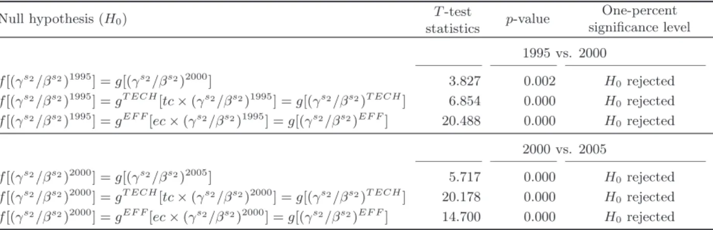
(7) case is also important because of the impact of the recent economic and financial crises on Spanish public sector deficit—which as of September, 2009, is roughly 6% of the GDP, whereas in 2007 there was a surplus. Compared to other European countries the scenario is gloomier with forecasts indicating it will take longer for the Spanish economy to surge again. In this difficult scenario, the relevance of the study on efficiency and related issues in the public sector gains momentum. The article is structured as follows. After this introduction, Sections 2 provides the methods used. Section 3 presents the data on inputs and outputs, while Section 4 shows the results. Finally, Section 5 presents some concluding remarks.. 2.. Methods. Our methods are based on the seminal ideas of Charnes et al. (1978), who developed Data Envelopment Analysis (DEA) to measure the technical efficiency of production. One of the main advantages of these methods is their absence of rigid assumptions. However, an even more flexible approach is Free Disposable Hull (FDH) in which the convexity assumption on the technology is dropped (Deprins et al., 1984). Our study uses this approach for both its higher flexibility and superior asymptotic properties (Park et al., 2000). We can also use some graphical examples to better realize the advantages of using FDH as opposed to DEA. Figure 1 depicts a scenario for five municipalities (A, B, C, D and E). For simplicity reasons, we assume that only one output y is produced (which is represented in the horizontal axis) while the vertical axis represents total costs (T C). In this example, irrespective of the convexity assumption, units A, B, C and D appear as efficient in their respective scale (say, they are efficient in the variable returns to scale, VRS, technology), while municipality E is inefficient, since it is possible to find a less costly way to produce the output level production y E . The standard (convex) VRS cost efficiency model will show that it is possible to produce y E with a lower total cost than the observed cost for municipality E (αDEA × T C E < T C E ). The cost efficiency coefficient αDEA will show a value lower than the unity, indicating the percentage of the observed cost to reach the convex frontier. In Figure 1 it is assumed than municipalities A and B are operating in a centralized environment (which we label S1 ), while municipalities C, D and E are operating in a decentralized environment (which we label S2 ). In these specific circumstances, the convexity assumption causes a problem because the point of the convex cost frontier to evaluate unit E requires a combination of units B and C which could be unfeasible because they are sit7.

(8) uated in different operating frameworks. Under these circumstances, the application of the non-convex (FDH) cost frontier offers a less controversial combination: unit E is inefficient because its total costs to produce y E are higher than αFDH × T C E , a cost reference taken from the existence of unit C. In this simple example, it is worth mentioning that part of the cost excess [(αFDH − αDEA ) × T C E ] hinges exclusively on the convexity assumption. In a previous study Balaguer-Coll et al. (2009) present a methodology to compare centralized (municipalities with less powers) and decentralized municipalities (with more powers). The main interest of their proposal was to enable comparison of decentralized municipalities with two reference points on the frontier, namely, one from the decentralized sub-sample (S2 ) of municipalities and the other from the centralized sub-sample (S1 ).2 Figure 2 depicts a hypothetical scenario where decentralized municipalities are more efficient than centralized when evaluating unit E. As can be seen, the total cost of cloning the centralized municipality A three times produces the output level y E with a cost frontier γ × T C E higher than the cost frontier coming from the frontier defined by the decentralized municipalities (β × T C E ) . Summing up, Figure 2 shows the scenario where decentralization economies dominate; under these circumstances, the ratio between the cost efficiency coefficients (γ/β) will be higher than the unity. However, nothing is granted in advance, as the opposite situation could also prevail. In Figure 3 we can see how the point on the frontier obtained by duplicating municipality A can produce y E with smaller total costs than the frontier defined by the decentralized municipalities (γ × T C E < β × T C E ). In this specific case, Figure 3 represents an example where centralized municipalities are operating with a better level of efficiency with respect to the decentralized municipalities. In this circumstance, the ratio between the cost efficiency coefficients (γ/β) will be smaller than the unity. 2.1.. Temporal analysis. The evaluation process represented in figures 1–3 has been developed in a previous article (Balaguer-Coll et al., 2009). We now present a natural extension introducing movements over time of the frontiers corresponding to both centralized and decentralized municipalities. Therefore, the question to answer is now different, since the objective is to ascertain to what extent differences in cost efficiency among centralized and decentralized municipalities are expanded or contracted between two periods t and t + 1. In other words, while in Balaguer2 Here we will only present the graphical illustration to offer an intuitive idea about their proposal. Programs [7] and [8] in Balaguer-Coll et al. (2009) define the mathematical programs that quantify coefficients β and γ.. 8.

(9) Coll et al. (2009) a static picture is presented, we now focus on sequence of movements, which is more complex as changes in time can be generated by a variety of causes. Let us therefore assume that we have data corresponding to two time periods (t and t + 1) for the two sub-samples of municipalities (those operating in a centralized environment, S1 , and those others operating in a decentralized system, S2 ). It is feasible to define an index evaluating the time evolution of the coefficients presented earlier as follows: γ s2 ,t+1 /β s2 ,t+1 γ s2 ,t+1 /γ s2 ,t = γ s2 ,t /β s2 ,t β s2 ,t+1 /β s2 ,t. (1). whose value will be above (below) unity when decentralization economies increase (decrease) between periods t and t + 1, respectively. If nothing changes, the index equals unity. This temporal index can be decomposed analogously to the Malmquist indices (see Caves et al., 1982; Grosskopf, 2003). In doing so, we determine the importance of technical change (frontier shifts between t and t + 1), and efficiency change (considering the movements in the distance separating the observation analyzed from their respective frontiers). Allowing for this decomposition involves defining two integer programming problems which combine information corresponding to periods t and t + 1: OE(ys2 ,t+1 ) = min β̃ s2 ,t+1 β̃,λ,z. s.t.. β̃ s2 ,t+1 T C s2,t+1. − TCs2 ,t λ ≥ 0,. −ys2 ,t+1 + Ms2 ,t λ ≥ 0, zB ≥ λ, − → 1 z = 1, z = {0, 1}, λ = integer, and. 9. (2).

(10) OE s2 (ys2 ,t+1 ) = min γ̃ s2 ,t+1 γ̃,λ,z. s.t.. γ̃ s2 ,t+1 T C s2 ,t+1. − TCs1 ,t λ ≥ 0,. −ys2 ,t+1 + Ms1 ,t λ ≥ 0, (3). zB ≥ λ, − → 1 z = 1, z = {0, 1}, λ = integer.. where y, TC , β and γ have been already defined and λ is an activity integer vector denoting the intensity levels at which the benchmark observation is conducted; M is a matrix containing the observed output vectors for the centralized (MS1 ) and decentralized (MS2 ) municipalities; z is an activity integer vector having a value equal to one when referring to the unit taken as a benchmark and having a null value otherwise; and B is a scalar with a large absolute value. Having obtained these new cost efficiency coefficients, it is a straightforward process to decompose the index in order to define the technical change and efficiency change components: γ s2 ,t+1 /β s2 ,t+1 γ s2 ,t /β s2 ,t ! "# $. Decentralization economies index. =. γ s2 ,t+1 /γ̃ s2 ,t+1 β s2 ,t+1 /β̃ s2 ,t+1 ! "# $. Technical change index (tc). ×. γ̃ s2 ,t+1 /γ s2 ,t β̃ s2 ,t+1 /β s2 ,t ! "# $. (4). Efficiency change index (ec). The technical change index (tc) quantifies the observed movements on the frontier of more decentralized municipalities with respect to the change in the frontier made up of less decentralized ones. This index encompasses the relative shifts in best-practice technology, corresponding to the two samples (S1 and S2 ) under analysis, between periods t and t + 1. A technical change index larger than unity indicates that the best practice frontier of subsample S2 improves more rapidly than that corresponding to sub-sample S1 (i.e., decentralized municipalities go through faster technical progress). When the technical change index is below unity, then the technical progress of the S1 sub-sample is higher than the technical progress corresponding to the sub-sample S2 (i.e., less decentralized municipalities experience faster technical progress). One empirical example sheds light on the interpretation of this component. If decentralization provides flexibility, and flexibility favors the capacity to innovate in order to do things better over time, then the technical change index is above unity when decentralized municipalities demonstrate to having introduced innovations better than non decentralized. 10.

(11) municipalities have. In contrast, the efficiency change index (or catching up effect, ec), shows what the changes in the relative cost efficiency levels are, corresponding to the two samples—S1 and S2 —under analysis, between periods t and t + 1. This index defines the distance of the observed costs for periods t and t + 1 with respect to the frontier in period t. It indicates whether observations in t + 1 are closer to the frontier than they are in period t. When the efficiency change index is larger than unity, the cost efficiency change between periods t and t + 1 shows greater improvement for S2 (decentralized) sub-sample than for the S1 (less decentralized) sub-sample. On the other hand, when the efficiency change index is below unity, the distance with respect to the frontier of the sub-sample S1 (less decentralized) increases more than the distance with respect to sub-sample S2 (decentralized). Following the example of decentralization as a way to introduce flexibility, the efficiency change index is above unity when decentralized municipalities which take advantage of their flexibility are able to emulate the best performers faster than non flexible municipalities. In other words, non decentralized municipalities face a kind of barrier to mobility that limits their capacity to adopt innovations. As suggested by Worthington and Dollery (2000), this distinction is important from a policy viewpoint, since the changes in productivity growth due to inefficiency demand different policies from those concerning technical change (see Grosskopf, 1993). As Worthington and Dollery (2000) indicate sluggish productivity due to a poor efficiency change index would require policies designed to foster innovations. In contrast, policies designed to innovate would exert its impact on the technical change index. 2.2.. Bipartite decomposition of the factors affecting the decentralization economies index. We now turn to an analysis of the distribution dynamics of the decentralization economies index, which is generally more informative than summary statistics such as the conditional mean of variance, especially when multi-modality is present. Our objective is to assess the degree to which each of the three components of productivity change account for deforming the distribution of the decentralization index between 1995 and 2000, and between 2000 and 2005, in a similar fashion as Kumar and Russell (2002). We carry out the analysis by considering nonparametric kernel-based density estimates of our decentralization indices. By rearranging terms in Equation (4) we obtain an expression which provides us with. 11.

(12) information for period t + 1 level of decentralization economies: (γ s2 /β s2 )t+1 = tc × ec × (γ s2 /β s2 )t. (5). where tc = (γ s2 ,t+1 /γ̃ s2 ,t+1 )/(β s2 ,t+1 /β̃ s2 ,t+1 ) are the changes in decentralization economies due to technological change (technical change index), ec = (γ̃ s2 ,t+1 /γ s2 ,t )/(β̃ s2 ,t+1 /β s2 ,t ) represents the changes in decentralization economies due to efficiency change (efficiency change index), and (γ s2 /β s2 )t represents the decentralization index in period t. Consequently, both tc and ec impact on the advance of γ s2 /β s2 . Both the effect of tc and ec can be measured. The distribution of the decentralization economies index in period t + 1 can consequently be constructed by successively multiplying the decentralization economies index in period t by each of the two factors, i.e., technical change and efficiency change. This in turn allows us to construct counterfactual distributions by sequential introduction of each factor. The counterfactual t + 1 period decentralization economies index distribution of the variable (γ s2 /β s2 )T ECH = tc × (γ s2 /β s2 )t. (6). isolates the effect on the distribution of changes in technology only, assuming that efficiency change is irrelevant. Therefore, the shift from (γ s2 /β s2 )t to (γ s2 /β s2 )t+1 would be induced by changes in technology. The counterfactual t + 1 period decentralization economies index distribution of the variable (γ s2 /β s2 )EF F = ec × (γ s2 /β s2 )t. (7). isolates the effect on the distribution of γ s2 /β s2 of changes in efficiency only, as if technical change were irrelevant. Therefore, the shift from (γ s2 /β s2 )t to (γ s2 /β s2 )t+1 would be induced by changes in efficiency only. As indicated above, this analysis is performed using kernel smoothing methods. The literature on this topic is voluminous, and several monographs provide appropriate in-depth analysis (see, for instance, Silverman, 1986). The recent monograph by Li and Racine (2007) is a nice compendium of previous studies, with new additional contributions. The general kernel estimator is the Rosenblatt (1956)-Parzen (1962) kernel estimator,. 12.

(13) whose expression is: fˆ(x) = (Sh)−1. S % s=1. S &x − x' % s −1 K = (Sh) K(ψs ) h. (8). s=1. where fˆ is the estimated density, x is the evaluation point, xs is the observation being evaluated (s = 1, . . . , S) and h is the bandwidth. When estimating a density function via kernel smoothing methods, two critical decisions must be made: (i) choosing the kernel; (ii) choosing the bandwidth. Both affect the shape of the density, but the effect of the second decision is much larger compared with the first one and, consequently, the literature devoted to the selection of bandwidth is vast. Regarding the choice of kernel, several alternatives are available. The features of a kernel are those of a density function, and thus, kernels are frequently chosen to be well-known density functions (Pagan and Ullah, 1999), for example the standard normal K(ψ) = (2π)−1/2 exp(−.5ψ 2 ), which was our choice. Regarding the bandwidth, we have considered plug-in methods (Sheather and Jones, 1991) because of their superior performance in terms of balance between bias and variance compared with other methods. We can also look at nonparametric techniques to formally test whether the distributions obtained in previous sections differ statistically. Specifically, we apply the Li (1996) test, which analyzes whether two unknown distributions differ significantly. Therefore, if f and g are the distributions corresponding to, let us say, γ s2 ,t /β s2 ,t and γ s2 ,t+1 /β s2 ,t+1 , the testable null hypothesis would be H0 : γ s2 ,t /β s2 ,t = γ s2 ,t+1 /β s2 ,t+1 against the alternative, H1 : γ s2 ,t /β s2 ,t &= γ s2 ,t+1 /β s2 ,t+1 .3 The test we use is based on the generally accepted idea of measuring the global distance (closeness) between two densities f (x) and g(x) by the integrated squared error (Pagan and Ullah, 1999). The integrated square error is the basis for constructing the statistic on which the test is based (see Fan, 1994; Li, 1996; Pagan and Ullah, 1999). The Li (1996) test requires some assumptions to be met such as independently distributed observations in each sub-group, and identically within each sub-group. However, our estimates are dependent in the statistical sense, since they have been obtained using linear programming methods. Therefore, perturbations of observations which lie on the estimated frontier will generally affect the efficiencies estimated for other observations. Under these circumstances it is not clear whether the Li (1996) test will perform satisfactorily. Accordingly, we follow Li (1999), 3. Some additional refinements to this test have been recently proposed; see, for instance Li et al. (2009).. 13.

(14) who shows that the bootstrap provides better inference than the standard normal. Simar and Zelenyuk (2006) stress this point, indicating that in the specific setup of efficiency scores obtained using linear programming techniques there is no real alternative to the bootstrap. Therefore, we adopt Simar and Zelenyuk’s (2006) proposal based on the bootstrap for adapting the Li (1996) test to the context of estimates obtained using linear programming methods. Specifically, consistent bootstrap estimates of the p-values of the Li (1996) test in its own specific context are provided by:. p̂ =. B 1 % ˆb ˆ I{J > J}, B. (9). b=1. where b = 1, . . . , B is the number of bootstrap replicates, I is an indicator function, Jˆ is the statistic yielded by the Li (1996) test, and Jˆb is the bootstrapped statistic. These p-values must be adapted to our context—where the true decentralization indices are replaced by our estimates from equations (2) and (3).. 3.. Data, inputs, and outputs. We use a sample of 1,164 Spanish municipalities with a population over 1,000 for years 1995, 2000 and 2005. Although the total number of municipalities in the database was higher, the final number of observations is lower because we consider only municipalities with available information for all sample years. Both input and output data are provided by the Spanish Ministry for Public Administration. The analysis is performed for 1995, 2000 and 2005 because the survey on local infrastructures and facilities (Encuesta de Infraestructuras y Equipamientos Locales), which provides information on outputs, is only available for those years. Input data has been constructed from local government budget information. The selection of outputs is based on the services and facilities provided by each municipality. Spanish local governments must provide minimum services depending on their number of inhabitants. Some of them are universally provided, yet others are only a legal requirement for larger municipalities. These categories are municipalities with: (i) less than 5,000 inhabitants; (ii) of over 5,000 and less than 20,000; (iii) of more than 20,000 and less than 50,000; (iv) and over 50,000. Our outputs have been selected according to the list of minimum services.4 They include population (Y1 ), number of lighting points (Y2 ), tons of waste collected 4. See Balaguer-Coll et al. (2009) for a detailed description of the minimum services that each category of municipalities must provide, and the output indicators designed to measure the different services.. 14.

(15) (Y3 ), street infrastructure (Y4 ), public buildings (Y5 ), market (Y6 ), public parks (Y7 ), and assistance centers (Y8 ). Outputs Y4 through Y8 are measured via their surface area, in square meters. We thus measure eight services by means of the proxy indicators. Using proxies is unavoidable since, as pointed out by De Borger and Kerstens (1996), population is clearly not a direct output of local production but is assumed to proxy for the various administrative tasks undertaken by municipalities. The choice has also been driven by previous studies on efficiency in other European local governments for which differences are basically confined to the area of education—in Spain it is controlled by higher levels of government. An interesting feature of our database is the inclusion of information on the quality of the infrastructures and facilities. This is measured using an indicator taking the value of 1 (bad), 2 (fair) or 3 (good). We have constructed a weighted indicator of average quality, and it has been modeled as an additional output (Y9 ).5 The choice of inputs is based on budget information, which reflects municipalities’ costs. Three main categories are included: current (ordinary) expenditures, capital expenditures, and financial expenditures. The first ones contain four further categories, which account for: (i) personnel expenditure; (ii) current goods and services expenditures; (iii) financial expenditures; (iv) current transfers. Capital expenditures are also decomposed, falling into either real investments, or capital transfers. The former is what the economic budgetary classification labels as capital expenditures, i.e., all expenditures local governments implement either: (i) to produce or acquire capital goods; (ii) to acquire necessary goods to provide local services in the right conditions; (iii) financial expenditures that are suitable for amortization. Capital transfers refer to the payments to institutions to finance certain investments. Since we measure overall cost efficiency, and all inputs refer to different costs’ categories, they have been added to sum up the total cost figure, T C.6 Some summary statistics for both inputs and outputs are reported in Table 1.. 4.. Results. The decentralization economies indicator should be interpreted as the gains that municipalities obtain over time from focusing on a wider range of services and facilities. Summary results are reported in Table 2, and they suggest that, over time—both from 1995 to 2000, and from 2000 to 2005—benefits are obtained from a broader range for municipalities with higher levels 5. The literature has considered multiple ways to control for the quality of the outputs. See, for instance, the early proposals by Banker and Morey (1986). 6 See Balaguer-Coll et al. (2009) for additional details on the inputs and budgetary classification.. 15.

(16) of powers, since most deciles of the decentralization economies index distribution present values greater than unity. We provide information for different deciles of the distribution, since it permits us to understand more accurately the magnitude of the decentralization economies. Globally, these results show that, in relative terms, the temporal evolution of decentralized (or devolved) municipalities improves on the cost frontier constructed with the less decentralized municipalities. The effect is not entirely mimicked for the 2000–2005, when the technical change effect still prevails yet to a lesser extent. However, the empirical evidence is not enough to conclude whether a clear tendency exists. Recall that expression (4) breaks down the decentralization economies index into two components: the technical change index (movements of the cost frontier) and the efficiency change index (change in the distance separating inefficiency units from their cost frontier). Table 2 is a good example of the advantages of breaking down global indices, in order to disentangle the extent to which there are basic phenomena probably masked by excessively aggregated indices. Indeed, the technical change index exhibits average values greater than unity, which indicates that the decentralized best performing municipalities have shifted their respective cost frontier more than the less decentralized best performers. On the other hand, as the efficiency change index is significantly smaller than unity, inefficient decentralized municipalities have been unable to follow the pace of the innovators. Therefore, the innovations introduced by decentralized municipalities have a remarkable impact on efficiency, but they encounter a sort of barriers to mobility, which hinders the spreading of these innovations among decentralized municipalities. Overall, this is reflected in that the scope for improving the efficiency of decentralized municipalities through innovations introduced by the most dynamic decentralized municipalities grew from 1995 to 2000, and to a lesser extent from 2000 to 2005. Regarding the inefficient units, once the barriers to mobility are overcome, they have a potential growth in efficiency and emulate the innovations introduced by the most dynamic decentralized municipalities. In sum, innovations producing shifts in the cost frontiers are far more important in decentralized municipalities. The shifts in the frontier, however, are not mechanically translated to the decentralization index because there seems to be a problem in the spread of innovations. Once the problem of how to disseminate these good practices is solved, the advantage of decentralized municipalities in dynamic terms would be unquestionable. We now turn to an analysis of distribution dynamics of the decentralization indices, and focus not only on summary statistics like those reported in Table 1, but on how the entire. 16.

(17) distributions have evolved. Figures 4 through 7 provide the means to assess to what extent each of the two components of the decentralization economies index—technical change and efficiency change—account for the deformation of its distribution between the selected subperiods and the entire 1995–2005 period. Figure 4.a displays kernel-based density estimates (essentially “smoothed” histograms) of γ s2 /β s2 for years 1995 (t, solid line) and 2000 (t + 1, dashed line). Figure 6.a reports analogous information for the 2000–2005 subperiod. Vertical lines represent mean values for each distribution in each figure, i.e., solid line for the base period, b, and dashed line for the current period, c. Both b and c differ for the different figures. In Figure 4 and Figure 5 b = 1995 and c = 2000, whereas in Figure 6 and Figure 7, b = 2000 and c = 2005. These vertical lines suggest that the advances have been modest and, therefore, we can probably conclude that decentralization economies have not improved over time on average. A more extended graphical analysis considering the entire distribution and not only a summary statistic reveals that differences between both distributions are not very important, and therefore we can probably conclude that decentralization economies have not improved over time. This conclusion applies for the 2000–2005 transition (Figure 6.a and Figure 7.a). However, for the 1995–2000 period (Figure 4.a and Figure 5.a) differences between both densities are peculiar, as we could conclude they are confined to being slightly tighter in year 2000. The bandwidths for the different densities (obtained using the second-generation plug-in method by Sheather and Jones (1991)) are reported in the different legends. Not all the legends have bandwidths, since some of the figures are the same.7 However, decomposing the evolution of γ s2 /β s2 into its two components (technical change and efficiency change) suggests the shift from γ s2 ,1995 /β s2 ,1995 to γ s2 ,2000 /β s2 ,2000 has been generated by two opposite effects. Figure 4.b indicates that the factor contributing positively to its advance has been a technical change component. The solid line represents the distribution in Equation (6), which isolates the effect on the distribution of changes in technology only, as if no efficiency change occurred from 1995 to 2000. Therefore, the final (year 2000) distribution would be represented by the solid line. Vertical lines indicate the mean values for both distributions (γ s2 ,1995 /β s2 ,1995 and (γ s2 /β s2 )T ECH = tc × (γ s2 /β s2 )1995 , respectively) do indeed differ substantially, as already reported in Table 1. What Table 1 does not indicate is that, although the technical change index has increased to a large extent, dispersion has also increased remarkably, as reflected by much more spread probability mass for (γ s2 /β s2 )T ECH as compared with γ s2 ,1995 /β s2 ,1995 . Finally, Figure 4.c displays the distribution of γ s2 /β s2 for 7. Figures and bandwidths obtained by alternative methods are available upon request. Results only differed slightly.. 17.

(18) year 2000 alone, i.e., transition from Figure 4.b to Figure 4.c reveals the effect of efficiency change only. The patterns are very similar when evaluating the transitions from 2000 to 2005 (Figure 6.b), except for the existence of certain bimodality from 1995 to 2000 (Figure 4.b). Therefore, the general trend—indicating that dispersion is much higher regarding technical change—is corroborated. It is also important to realize the importance of evaluating these trends not only via the usual summary statistics (mean and standard deviation) but rather examining the shape of the densities. Their analysis is important because of their peculiarities, showing that the effect of technical change leads to its flattening, especially in the vicinity of the average. Figure 5 and Figure 7 report similar information to that reported in Figure 4 and Figure 6, respectively. The main difference is contained in Figure 5.b and Figure 7.b, where the solid lines indicate what the impact is on γ s2 /β s2 of efficiency change only, i.e., we isolate the effect on the distribution of γ s2 /β s2 as if no technical change existed. As indicated by both the mean (solid vertical line) and the deformation of the distribution, it is clearly detrimental, for both 1995–2000 (Figure 5.b) and 2000–2005 (Figure 7.b) periods. The decline in the mean value is lower than the mean increase reported in Figure 4.b and Figure 6.b, and insinuates that a positive effect over time could prevail. However, as shown by Figure 4.a and 5.a, the shapes of the distributions do not seem to differ a great deal. The conclusions inferred from visually analyzing distributions can be reinforced via application of the tests proposed in Section 2 (Li, 1996, 1999; Simar and Zelenyuk, 2006). These are reported in Table 3, which corroborate results in figures 4 through 7. The p-values obtained when testing the null H0 : f [(γ s2 /β s2 )b ] = g[(γ s2 /β s2 )c ] indicates that the visual differences found between distributions in the base (b) and current (c) periods are significant in all instances. Therefore, the effects of technical change and efficiency change considered individually lead to significant changes in the shape of the densities, since both of them are statistically significant at the most stringent significance levels and for all comparisons (either 1995 vs. 2000, or 2000 vs. 2005).. 5.. Concluding remarks. In this article we analyze the links between devolution and efficiency of Spanish municipalities from a dynamic perspective, considering the evolution for two periods, namely, from 1995 to 2000, and from 2000 to 2005. These are relevant years in which the Spanish economy surged, and when some relevant initiatives for Spanish local governments took place. We 18.

(19) construct a methodology based on the (deterministic) frontier production function literature (Farrell, 1957; Afriat, 1972; Färe et al., 1994). Specifically, we derived an indicator à la Malmquist (Caves et al., 1982) which allows us to measure whether efficiency gains from enhanced decentralization of powers have increased over time. The indicator also decomposes this time evolution in two components with specific economic meanings, in a similar fashion to the Malmquist index which decomposes productivity change into efficiency change and technical change. We also consider a sequential decomposition of the decentralization economies indicator in the spirit of Kumar and Russell (2002). This decomposition allows us to ascertain what the most important component of the decentralization economies indicator is—either the technical change or the catching up component. We consider that this methodology is important since results might vary a great deal across local governments, and applying this approach generates results which are not based on central moments of the distribution only. In particular, results show that the effect of technical change varies a great deal across municipalities, whereas catching up is more homogeneous. The application to Spanish local governments is relevant for several reasons, among which we may highlight the debate on the hypothetical benefits attainable from a second decentralization (that consists of transferring powers not only from national to regional but also from regional to the lowest level of government, i.e., municipalities), and the response of municipalities to the new regulatory environment emerging after passing the law on the balanced budget, which is related to the European Stability and Growth Pact. Some recent trends in the economy such as the crisis of the construction sector make it even more relevant to analyze the Spanish case, where powers related to urbanism are in hands of municipalities. Results show that, over time, benefits for larger municipalities (with more powers) are increasing, due to the relatively higher magnitude of the technical change compared to the efficiency change index. However, differences are remarkable across municipalities—some of them perform very well, others trail behind. Decentralization economies, which are the result of the combined effect of technical change and efficiency change, have not improved on average, and this result is robust to the period under analysis—either 1995–2000 or 2000–2005. In contrast, efficiency change is lower, but differences among municipalities are less stringent, contributing positively to reduce discrepancies among municipalities in the decentralization index. These findings could be related to the trend experienced in most public sector areas before Spain’s economy joined the Euro, which followed the stipulations of the Maastricht. 19.

(20) Treaty on the sustainability of the government’s financial position. The commitments of Maastricht brought about a policy of deficit control, boosting the demand for more efficient government and public administration, and a “White paper on the improvement of public services. A new administration at the service of citizens” was released in 1999. These were initiatives to reform public administration, introducing many of the specific changes in management practice, included in the New Public Management (NPM) (Pollitt, 2002) recipe, but without being able to set off systemic changes. Thus, although Spain has implemented many of the ingredients of the NPM, there are still few visible benefits. Our findings, indicating that remarkable differences exist between municipalities, corroborate these claims. They also confirm that trends differ for the two sample periods considered, although only slightly. In line with the implications pointed out by Worthington and Dollery (2000), our results show technical progress together with negative efficiency change. This means that specific decentralized municipalities (those that operate efficiently) might be innovating and taking advantage of their new management practices. However, during the period we analyze the spread of innovations does not occur at the same pace (this duality is more evident in the period 1995–2000 than in 2000–2005). The improvement in the level of decentralized municipalities’ efficiency will therefore depend more on the spread of existing innovations to inefficient municipalities—a kind of contagion from the innovators to the inefficient followers—than in the generation of additional ones. This process can be reinforced by disseminating among local governments those reforms that were introduced and have shown positive results.. 20.

(21) References Afriat, S. (1972). Efficiency estimation of production functions. International Economic Review, 13:568–598. Akai, N. and Sakata, M. (2002). Fiscal decentralization contributes to economic growth: evidence from state-level cross-section data for the United States. Journal of Urban Economics, 52(1):93–108. Balaguer-Coll, M. T., Prior, D., and Tortosa-Ausina, E. (2009). Decentralization and efficiency of local government. The Annals of Regional Science, forthcoming. Banker, R. D. and Morey, R. C. (1986). The use of categorical variables in Data Envelopment Analysis. Management Science, 32:1613–1627. Barankay, I. and Lockwood, B. (2007). Decentralization and the productive efficiency of government: Evidence from Swiss cantons. Journal of Public Economics, 91(5-6):1197–1218. Cai, H. and Treisman, D. (2004). State corroding federalism. Journal of Public Economics, 88:819–843. Calamai, L. (2009). The link between devolution and regional disparities: evidence from the Italian regions. Environment and Planning A, 41(1). Caves, D. W., Christensen, L. R., and Diewert, W. E. (1982). The economic theory of index numbers and the measurement of input, output, and productivity. Econometrica, 50(6):1393–1414. Charnes, A., Cooper, W. W., and Rhodes, E. (1978). Measuring the efficiency of decision making units. European Journal of Operational Research, 2(6):429–444. Davoodi, H. and Zou, H. (1998). Fiscal decentralization and economic growth: A cross-country study. Journal of Urban Economics, 43(2):244–257. De Borger, B. and Kerstens, K. (1996). Cost efficiency of Belgian local governments: A comparative analysis of FDH, DEA, and econometric approaches. Regional Science and Urban Economics, 26:145–170. Deprins, D., Simar, L., and Tulkens, H. (1984). Measuring labor-efficiency in post offices. In Marchand, M., Pestieau, P., and Tulkens, H., editors, The Performance of Public Enterprises: Concepts and Measurement, chapter 10, pages 243–267. North-Holland, Amsterdam. Fan, Y. (1994). Testing the goodness-of-fit of a parametric density function by kernel method. Econometric Theory, 10:316–356. Färe, R., Grosskopf, S., and Lovell, C. A. K. (1994). Production Frontiers. Cambridge University Press, Cambridge.. 21.

(22) Farrell, M. J. (1957). The measurement of productive efficiency. Journal of the Royal Statistical Society, Ser.A,120:253–281. Grosskopf, S. (1993). Efficiency and productivity. In Fried, H. O., Lovell, C. A. K., and Schmidt, S. S., editors, The Measurement of Productive Efficiency: Techniques and Applications, chapter 4, pages 161–193. Oxford University Press, Oxford. Grosskopf, S. (2003). Some remarks on productivity and its decompositions. Journal of Productivity Analysis, 20:459–474. Iimi, A. (2005). Decentralization and economic growth revisited: an empirical note. Journal of Urban Economics, 57(3):449–461. Inman, R. and Rubinfeld, D. (1997). Rethinking federalism. The Journal of Economic Perspectives, 11(4):43–64. Inman, R. and Rubinfeld, D. (1998). Subsidiarity and the European Union. Working Paper 6556, NBER, Cambridge, MA. Keating, M. (1998). The New Regionalism in Western Europe: Territorial Restructuring and Political Change. Edward Elgar, Northampton. Klugman, J. (1994). Decentralisation: A survey of literature from a human development perspective. Development Programme Occasional Paper 13, United Nations, Human Development Report Office, New York. Kumar, S. and Russell, R. R. (2002). Technological change, technological catch-up, and capital deepening: Relative contributions to growth and convergence. American Economic Review, 92(3):527–548. Li, Q. (1996). Nonparametric testing of closeness between two unknown distribution functions. Econometric Reviews, 15:261–274. Li, Q. (1999). Nonparametric testing the similarity of two unknown density functions: local power and bootstrap analysis. Journal of Nonparametric Statistics, 11(1):189–213. Li, Q., Maasoumi, E., and Racine, J. S. (2009). A nonparametric test for equality of distributions with mixed categorical and continuous data. Journal of Econometrics, 148(2):186–200. Li, Q. and Racine, J. S. (2007). Nonparametric Econometrics: Theory and Practice. Princeton University Press, Princeton and Oxford. Lin, J. Y. and Liu, Z. (2000). Fiscal decentralization and economic growth in China. Economic Development and Cultural Change, 49(1):1–21.. 22.

(23) Martinez-Vazquez, J. and McNab, R. (2003). Fiscal decentralization and economic growth. World Development, 31(9):1597–1616. Núñez, X. M. (2001). What is Spanish nationalism today? From legitimacy crisis to unfulfilled renovation (1975-2000). Ethnic and Racial Studies, 24(5):719–752. Oates, W. E. (1972). Fiscal Federalism. Harcourt Brace Jovanovich, Inc., New York. Pagan, A. and Ullah, A. (1999). Nonparametric Econometrics. Themes in modern econometrics. Cambridge University Press, Cambridge. Park, B. U., Simar, L., and Weiner, C. (2000). The FDH estimator for productivity efficiency scores. Econometric Theory, 16(6):855–877. Parzen, E. (1962). On estimation of a probability density function and mode. Annals of Mathematical Statistics, 33:1065–1076. Peterson, P. E. (1981). City Limits. University of Chicago Press, Chicago. Pollitt, C. (2002). The New Public Management in International Perspective. New public management: Current trends and future prospects, page 274. Prud’homme, R. (1995). The dangers of decentralization. World Bank Research Observer, 10:201–220. Rodríguez-Pose, A. (1996). Growth and institutional change: the influence of the Spanish regionalisation process on economic performance. Environment and Planning C, 14:71–88. Rodríguez-Pose, A. and Bwire, A. (2004). The economic (in)efficiency of devolution. Environment and Planning A, 36(11):1907–1928. Rodríguez-Pose, A. and Gill, N. (2005). On the ‘economic dividend’ of devolution. Regional Studies, 39(4):405–420. Rodríguez-Pose, A., Tijmstra, S. A., and Bwire, A. (2009). Fiscal decentralisation, efficiency, and growth. Environment and Planning A, 41(9):2041–2062. Rosenblatt, M. (1956). Remarks on some non-parametric estimates of a density function. The Annals of Mathematical Statistics, 27:832–837. Sheather, S. J. and Jones, M. C. (1991). A reliable data-based bandwidth selection method for kernel density estimation. Journal of the Royal Statistical Society, Ser.B,53(3):683–690. Silva-Ochoa, E. (2009). Institutions and the provision of local services in Mexico. Environment and Planning C: Government & Policy, 27(1):141–158.. 23.

(24) Silverman, B. W. (1986). Density Estimation for Statistics and Data Analysis. Chapman and Hall, London. Simar, L. and Zelenyuk, V. (2006). On testing equality of distributions of technical efficiency scores. Econometric Reviews, 25(4):497–522. Stewart, K. (2000). Fiscal Federalism in Russia: Intergovernmental Transfers and the Financing of Education. Edward Elgar Publishing. Thießen, U. (2003). Fiscal decentralization and economic growth in high-income OECD countries. Fiscal Studies, 24(3):237–274. Thornton, J. (2007). Fiscal decentralization and economic growth reconsidered. Journal of Urban Economics, 61(1):64–70. Tiebout, C. (1956). A pure theory of local expenditures. Journal of Political Economy, 64:416–424. Worthington, A. C. and Dollery, B. (2000). An empirical analysis of productivity change in Australian local government, 1993/94 to 1995/96. Working Paper Series in Economics 2000–3, University of New England, School of Economic Studies. Xie, D., Zou, H., and Davoodi, H. (1999). Fiscal decentralization and economic growth in the United States. Journal of Urban Economics, 45(2):228–239. Zhang, T. and Zou, H. (1998). Fiscal decentralization, public spending, and economic growth in China. Journal of Public Economics, 67(2):221–240. Zhang, T. and Zou, H. (2001). The growth impact of intersectoral and intergovernmental allocation of public expenditure With applications to China and India. China Economic Review, 12(1):58–81.. 24.

(25) Table 1: Summary statistics for inputs and outputs, year 2005) Median. Inputs a,b. Total costs. (T C). Std.Dev.. 669.999. 441.280. 3,290.500 0.233 0.467 51.966 0.028 0.002 3.373 0.170 2.283. 8,935.361 1.355 34.985 41.255 1.784 3.077 204.229 0.766 0.315. Outputs Population (Y1 ) Number of lighting pointsb (Y2 ) Tones of waste collectedc (Y3 ) Street infrastructure surface areab,c (Y4 ) Public buildings surface areab,c (Y5 ) Market surface areab,c (Y6 ) Registered area of public parksb,c (Y7 ) Assistance centers surface area b,c (Y8 ) Quality (Y9 ) # of observations a b c. 1,164. In thousands of 1995 pesetas (1 euro=166.386 pesetas). Divided by population. In square metres.. 25.

(26) Table 2: Percentage change of bipartite decomposition indexes, selected deciles Index. 10% decile. 30% decile. 50% decile (median). 70% decile. 90% decile. 124.10 186.23 93.01. 228.77 311.24 153.80. 113.07 153.77 100. 162.87 270.30 128.18. 1995–2000. 26. Change in decentralization economies Technical change Efficiency change. 52.05 77.71 29.73. 76.92 107.08 52.78. 96.03 142.20 70.11 2000–2005. Change in decentralization economies Technical change Efficiency change. 34.49 48.65 39.25. 71.59 86.07 60.95. 89.51 112.98 80.76.

(27) Table 3: Distribution hypothesis tests, 1995 vs. 2000 vs. 2005 (Li, 1999; Simar and Zelenyuk, 2006) T -test statistics. Null hypothesis (H0 ). p-value. One-percent significance level. 1995 vs. 2000. 27. f [(γ s2 /β s2 )1995 ] = g[(γ s2 /β s2 )2000 ] f [(γ s2 /β s2 )1995 ] = g T ECH [tc × (γ s2 /β s2 )1995 ] = g[(γ s2 /β s2 )T ECH ] f [(γ s2 /β s2 )1995 ] = g EF F [ec × (γ s2 /β s2 )1995 ] = g[(γ s2 /β s2 )EF F ]. 3.827 6.854 20.488. 0.002 0.000 0.000. H0 rejected H0 rejected H0 rejected. 2000 vs. 2005 s2. s2 2000. s2. s2 2005. f [(γ /β ) ] = g[(γ /β ) ] s2 s2 2000 T ECH s2 f [(γ /β ) ]=g [tc × (γ /β s2 )2000 ] = g[(γ s2 /β s2 )T ECH ] s2 s2 2000 EF F f [(γ /β ) ]=g [ec × (γ s2 /β s2 )2000 ] = g[(γ s2 /β s2 )EF F ]. 5.717 20.178 14.700. 0.000 0.000 0.000. H0 rejected H0 rejected H0 rejected. Notes: The functions f (·) and g(·) are (kernel) distribution functions for the actual decentralization economies index in the current and base period, respectively; g T ECH (·) and g EF F (·) are counterfactual distributions obtained by adjusting the 1995 distribution of (γ s2 /β s2 ) for the effects of advances in technology (tc) and advances in efficiency (ec), respectively..

(28) Figure 1: DEA vs. FDH frontier. • • • • •. 28.

(29) Figure 2: Scenario 1. Decentralized municipalities more efficient than centralized municipalities. • •. • •. • •. 29.

(30) Figure 3: Scenario 2. Centralized municipalities more efficient than decentralized municipalities. •. •. • • • •. 30.

(31) 1.5. 1.0. 0. 1. 2 3. 0. 1. 2 3. (b) Effect of technical change. 0. - - - - (γ s2 /β s2 )2000 , h = .1042 ——– tc × (γ s2 /β s2 )1995 , h = .1898. - - - - (γ s2 /β s2 )2000. 0. 2. ——– ec × tc × (γ s2 /β s2 )1995. 1. - - - - (γ s2 /β s2 )2000. 1. 2 3. (a) Actual γ s2 /β s2 distributions. 0. 1. 2. 3. (b) Effect of efficiency change. ——– (γ s2 /β s2 )1995 , h = .1603. - - - - (γ s2 /β s2 )2000 , h = .1042. ——– ec × (γ s2 /β s2 )1995 , h = .0850. - - - - (γ s2 /β s2 )2000. 0. 3. (c) Effect of efficiency change. 2. ——– tc × ec × (γ s2 /β s2 )1995. 1. - - - - (γ s2 /β s2 )2000. 3. (c) Effect of technical change. Figure 5: Counterfactual distributions of the decentralization economies index, efficiency change effect, 1995–2000. ——– (γ s2 /β s2 )1995 , h = .1603. 0.5. 1.5. 0.5. 0.0. 1.0. 1.5. Density. 1.5 1.0. 0.0. Density 0.5. 1.0. 1.5 1.0. 0.0. Density. (a) Actual γ s2 /β s2 distributions. Density 0.5 0.0. 1.0. 1.5. Figure 4: Counterfactual distributions of the decentralization economies index, technical change effect, 1995–2000. Density 0.5 0.0. Density 0.5 0.0. 31.

(32) 1.5. 1.0. 0. 1. 2 3. 0. 1. 2 3. (b) Effect of technical change. 0. - - - - (γ s2 /β s2 )2005 , h = .0673 ——– tc × (γ s2 /β s2 )2000 , h = .1373. - - - - (γ s2 /β s2 )2005. 0. 2. ——– ec × tc × (γ s2 /β s2 )2000. 1. - - - - (γ s2 /β s2 )2005. 1. 2 3. (a) Actual γ s2 /β s2 distributions. 0. 1. 2. 3. (b) Effect of efficiency change. ——– (γ s2 /β s2 )2000. - - - - (γ s2 /β s2 )2005. ——– ec × (γ s2 /β s2 )2000 , h = .0636. - - - - (γ s2 /β s2 )2005. 0. 3. (c) Effect of efficiency change. 2. ——– tc × ec × (γ s2 /β s2 )2000. 1. - - - - (γ s2 /β s2 )2005. 3. (c) Effect of technical change. Figure 7: Counterfactual distributions of the decentralization economies index, efficiency change effect, 2000–2005. ——– (γ s2 /β s2 )2000 , h = .0807. 0.5. 1.5. 0.5. 0.0. 1.0. 1.5. Density. 1.5 1.0. 0.0. Density 0.5. 1.0. 1.5 1.0. 0.0. Density. (a) Actual γ s2 /β s2 distributions. Density 0.5 0.0. 1.0. 1.5. Figure 6: Counterfactual distributions of the decentralization economies index, technical change effect, 2000–2005. Density 0.5 0.0. Density 0.5 0.0. 32.

(33)