Determinants of the current account for a group of European countries

Texto completo

(1)UNIVERSITAT JAUME I. FINAL DEGREE PROJECT DETERMINANTS OF THE CURRENT ACCOUNT FOR A GROUP OF EUROPEAN COUNTRIES. SHEILA CURTO SASTRE [email protected] MARIAM CAMARERO OLIVAS ECONOMICS 2015.

(2) ABSTRACT. This paper has tried to find some of the determinants of the current account in six European countries to try to explain why some of them have surpluses and other current account deficit. By regressing six explanatory variables they were obtained those with greater significance for each country. The results show a heteroskedasticity between countries which helps to understand the different current account balances. This divergence between the significant variables of each of the countries listed as the macroeconomic policies adopted by each of the countries during these 41 years are generating so different current account balances.. JEL: E3, E4, E5, F5, F6.. 1.

(3) INDEX. 1. INTRODUCTION ……………………………………………………………………...4 2. STYLIZED FACTS...............................................................................................5 3. DATA AND EMPIRICAL FRAMEWORK…………………………………………..14 3.1.. OUR MODEL…………………………………………………………………17. 4. REGRESSION ……………………………………………………………………….27 4.1.. RESULTS OBTAINED IN GENERAL REGRESSION…………………..27. 4.2.. RESULTS OBTAINED IN THE TIME SERIES-APPROACH…………..29. 4.3.. SPECIFICATION TEST……………………………………………………33. 4.3.1. Lack of correlation………………………………………………………33 4.3.2. Lack of heteroskedasticity……………………………………………...34 4.3.3. Stationarity……………………………………………………………….34 5. CONCLUSION ……………………………………………………………………….36 6. REFERENCES ………………………………………………………………………37. TABLES. Table 1. Ratio Ca / GDP of some European countries…………………………………….8 Table 2. Variables used in the model………………………………………………………18 Table 3. FE panel robust regression………………………………………………………28 Table 4. Individual regressions for each country………………………………………….30 Table 5. Summary of significant variables for each country …………………………….33 Table 6. Correlation Test…………………………………………………………………….34 Table 7. White Test…………………………………………………………………………..34 Table 8. DFA Test…………………………………………………………………………….35. 2.

(4) GRAPHICS Figure 1. Chinese GDP growth compared with other countries…………………………..6 Figure 2. Current account balance US………………………………………………………7 Figure 3. Evolution of international capital flows to GDP………………………………...10 Figure 4. Composition of the bond portfolio based on maturity…………………………11 Figure 5. Evolution of Spanish debt………………………………………………………..12 Figure 6. Evolution of Greek debt…………………………………………………………..12 Figure 7. Evolution of Irish debt…………………………………………………………….13 Figure 8. Growth of the euro against the dollar in 2011………………………………….16 Figure 9. Growth of the euro against the dollar in 2015………………………………….17 Figure 10. Evolution of openness in European countries………………………………..19 Figure 11. Evolution of the real effective exchange rate…………………………………21 Figure 12. Accumulation of public deficits in European countries………………………22 Figure 13. Net foreign assets in some European countries……………………………..23 Figure 14. Interest rate developments of ten-year bonds in some European countries……………………………………………………………………………………….24 Figure 15. Evolution of oil prices over the last 30 years…………………………………25 Figure 16. Real price of oil over the last 15 years………………………………………..26. 3.

(5) 1. INTRODUCTION. In a globalized world in which we live numerous factors are influencing the various economies. The opening of borders, both physical and legal, has produced large economic changes. In this paper we analyse some of the factors with the greatest impact on the current account balance in several European countries. Our purpose is trying to explain in greater depth the variables that affect the balance of the current account of Germany, Finland, Belgium, Spain, Ireland and Greece. Additionally attempt to quantify the extent it affects later to make a comparison between countries. Numerous existing works related to the analysis of the variables of the current account, but in this case we decided to focus on six countries whose historical current account balances are very different. Thus we wanted to determine which variables influence the final balance to get the current account of each of the countries and therefore an explanation of the diversity of the results of the current accounts of European countries considered as homogeneous economies mostly. To carry out this work we have relied on some of the economic works done previously. Among them we have decided to highlight the most influential. Chin and Pasard (2003) make a great contribution on the medium-term determinants of the current account in the developed economies. The data range of our work ranges from 1970-2011, which were extracted from the database created by Catao and Milesi-Ferretti (2014), used in his work "External liabilities and crises", published that same year. From the database we decided to choose only those variables that conformed more to the purpose of our work. Many prior to the execution of our work on skills mismatches balances and current accounts were acquired from reading the work called "External adjustment global imbalances and valuation effects" (2013).. 4.

(6) 2. STYLIZED FACTS Before beginning we must consider some circumstances of the world around us to get in position, since over the years the world has experienced many changes and many high impacting modifications. Among them we decided to pick five: 1. In recent years, the global economic structure has undergone great changes. Since the beginning of trade liberalization, the US had held the top spot as the world's largest economy, but over the years and after the great awakening of the Asian giant, China, this position is more contested. China has experienced extraordinary economic growth in a relatively short time. In the Figure 1, we can see a comparison of growth of real GDP per capita in the period between 1998 and 2010. This data includes US, the Eurozone, Japan, Australia, UK, New Zealand and China. We can see how all countries follow similar growth rates, which have an index of almost complete convergence. Instead, China has stratospheric growth levels, far removed from the rest. Starting in 1998 with an index equal to 100, in just a few years China had already taken off their economic growth, arriving in 2010 to reach more than 300 points, while other countries were located about 125 points. In recent years China has managed to grow by 8 percentage points of GDP per year, with some years as in 2007 with an annual growth reached 14.2%.. 5.

(7) Figure 1. Chinese GDP growth compared with other countries. Due to its strong economic growth, China, like many other Asian countries became creditor to the rest of the world. In the case of the US, China is the holder of more than 7% of total US debt, making it the third creditor surpassed only by the US Social Security Fund and the Federal Reserve. Among the list of creditors of the US debt other Asian countries are located in the top fifteen, such as Japan in fifth place and Taiwan in the fifteenth. In the case of Spain, its main creditors are in first position in France, but again closely followed by China, which possesses more than 18% of public debt. 2. USA, known as the leading world power both its strong economy as being considered one of the most advanced countries in the world, has held the position as a net importer of capital since 1982. As we can see in the Figure 2, US has traditionally had current account deficit, which began in 1982 and has endured until today. Far from improving the situation, over the years it became worse, until reaching its peak in 2008 following the financial crisis, seems to have recovered the economy in recent years, the balance is still negative balance but a lower amount. 6.

(8) Figure 2. Current account balance US. For European countries we can find all kinds of balances on current accounts in different countries. According to historical balances we find three types of countries: first, those countries that have traditionally had a creditor position, i.e., its ca / GDP ratio always had positive values such as Finland and Denmark. Second, we find countries that have always received negative values in the cc / GDP as in the case of Spain and Greece ratio. Thirdly, we have countries that over time have suffered and whose fluctuations ca / GDP ratio has obtained positive or negative values depending on the year, including Germany. The values of ca / GDP ratio of some European countries previously mentioned, these data are collected from 1990 to 2006 are displayed.. 7.

(9) Table 1. Ratio Ca / GDP of some European countries.. Source: OCI. 8.

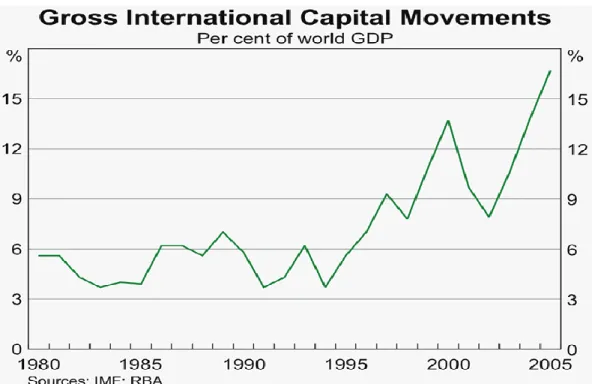
(10) The net value of current accounts of most developed countries have been declining in recent years, largely caused by the outbreak of the crisis in 2008. This has led to growing countries should borrow more to compensate balances. Another reason that surrounds this event is the grand opening of capital markets experienced in the last decade, making it easier to all economies access to more capital. 3. One of the major economic events of the last decades has experienced great liberalization in the capital market. Since 1990 there was experienced a big change in the regulations, which produced a large reduction in transaction costs and the easing of the current regulation. All these changes resulted in a large increase in capital flows, but this increase occurred with different intensity in all countries, in fact we can find big differences between the more developed and those that are in the process of developing economies. In the case of the European Union, following the Single European Act in 1992, there was the creation of a large European single market to comply with objectives including the free movement of capital was. But the release of the European capital market goes back a long time ago, 1960 to be exact. In this first phase of deregulation was "unconditionally liberalized direct investments, credits the short to medium term for commercial transactions and acquisitions of securities traded on the stock exchange. Without waiting for the EU decision, some Member States adopted unilateral national measures, which were suppressed by virtually all restrictions on capital movements. This was the case of the German Federal Republic in 1961, the UK in 1979, and the Benelux countries (including) in 1980. Later another Directive (72/156 / EEC) on international financial flows would be adopted "(Kolassa, 2015). Later, in 1985 and 1986 two new regulations expanding the degree of freedom were drafted, but some more efforts to carry out the dream of a single market were still needed, so subsequently two directives were drafted to reach full liberalization of the capital market. In the Figure 3, we can see how they have evolved capital flows to GDP in 25 years during the period between 1980 and 2005. Clearly we see a significant increase in gross international capital flows. In 1980 barely they reached 5 percentage points to GDP, while in 2005, before the outbreak of the financial. 9.

(11) crisis years, was achieved over 16% of GDP. So in just 25 years it was possible to triple the flow of capital. Figure 3. Evolution of international capital flows to GDP.. 4. The composition of the foreign assets of the country is often very heterogeneous. We can find big differences between developed countries and those that are under development. The former tend to opt for a kind of longterm risk, while the latter do so for a type of short-term risk. In the case of countries outside the European Union it that there is a high level of homogeneity, since they all have a composition very similar risk. Nearly 75% of its assets are sovereign, which have a very low risk level. On the other hand we have to evaluate the duration of the assets, which is also standard in all European countries. At European level, 25.1% of assets have duration of between 1 and 2 years, the most numerous. Moreover, they are also abundant those whose duration is between 1 and 3 months, occupying 13.7% of the total. By contrast, the rarer are those with duration of between 3 and 5 years, which represent only 1.2%.. 10.

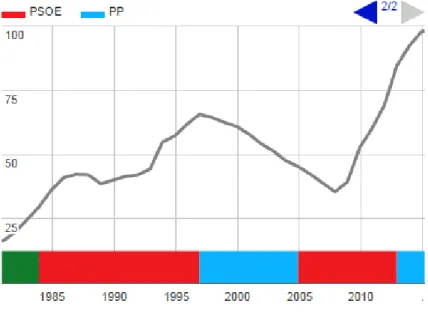
(12) Figure 4. Composition of the bond portfolio based on maturity. COMPOSITION BY MATURITY. Source: BCE. 5. The valuation effects are very important because we must take into account whether the positions held by individual countries on their gross external assets and liabilities account for their profits or losses. The most prominent example is the quintessential case of the United States, which has occupied a debit position for more than 30 years he has reported profits. In Europe, following the crisis we have aggravated the differences between countries. One of the countries to note is Spain, which at the end of 2014 had accumulated a debt of over 1.4 billion, ranking it as the second most indebted country in the world, behind only the US. In the Figure 5 we can see the evolution of the accumulated debt to GDP over the last 35 years. We see that Spain reached its lowest debt in 2007 when it represented just 35.5% of GDP. With the outbreak of the debt crisis began to rise uncontrollably into a very short period of time, reaching a record high in 2014 when it grew to more than 100% of GDP.. 11.

(13) Figure 5. Evolution of Spanish debt.. Source: datosmacro.com. Other European country to highlight is Greece, which has suffered a major impact due to the financial crisis, which has left the Greek economy to the brink of bankruptcy. As shown in the Figure 6 the increase in debt to GDP of the Hellenes it has been gradual, reaching in the years before the crisis one 103.10%, which is a very high figure considering that we were in the shock of the economic cycle. At this point, the Greek debt experienced a growth spurt in just seven years grew by more than 70 percentage points. Figure 6. Evolution of Greek debt.. Source: datosmacro.com. 12.

(14) Finally, the last European country to note is Ireland, which was also one of the greatest hit by the financial crisis, as in previous years had experienced a housing bubble like Spain. Ireland's case resembles that of Spain, since this country in the years before the crisis to reach its record low debt to GDP, as in 2007 he came to have only 24%. With the outbreak everything changed, he began suddenly increased debt in no time. In just seven years, Ireland went from a debt represented 24% of GDP in 2013 to have a 123.3% that quintupled the debt level. Besides all this, we must take into account that countries must deal with the payment of own debt interest, which represent large amounts of money annually.. Figure 7. Evolution of Irish debt.. Source: datosmacro.com. 13.

(15) Besides all this, we must take into account that countries must deal with the payment of own debt interest, which represent large amounts of money annually. In the case of Spain, the payment of debt interest forecast for the year 2015 is 31,650 million euros, or what the same 2.9% of GDP is. To this end Spain will grow at a rate of 2.9% for no longer accumulating more debt amount.. 3. DATA AND EMPIRICAL FRAMEWORK The data of a total of six countries will be discussed in this work, three of them with a debit balance in their current account and three with a credit balance included. As we have said before, these countries are Germany, Denmark, Finland, Spain, Greece and Ireland. The first three will be part of the group of countries with current account credit balance, while the next three will be in the group balance due. The period between 1970 and 2011 will be analysed with this data. In this period are included the last three crises that appeared in the European continent. In 1973, a global crisis emerged, caused mainly by the rise in oil prices.The oil-exporting countries decided to carry out a boycott of all those countries that had supported Israel during the Yom Kippur War. The rapid increase in the price of this product caused a strong inflationary effect and reduction in economic activity in countries with great energy dependence. Later in 1993 a great crisis emerged in Spain. It had dire consequences on levels of unemployment, which doubled in a period of very short time. Finally, as we all know, the worst finance crisis in the last 100 years appeared in the world, in October 2007. This crisis began as a result of the bursting of the housing bubble generated in the US, and expanded to the whole world through the very famous Subprime mortgages. The process of change to which the European Union has undergone in recent years should be mentioned. The most important point is undoubtedly the monetary union including today to a total of 19 countries. This monetary union has brought great changes in all nations whose have decided to join it, and the rest of the world.. 14.

(16) Before beginning, must be mentioned that all those countries that want to adhere to the introduction of the euro or would like to join in the future must meet preconditions. These conditions were called Maastricht convergence criteria. These criteria include the following: -. Domestic price stability, inflation cannot be higher than 1.5% of the average of the three members of the group with the lowest inflation.. -. The national nominal interest rate must be less than 2% of the average of the three countries in the group with the lowest interest rate.. -. The national debt should be less than 60% of GDP, in the event that this percentage is exceeded should be on the way to approach this value.. -. The deficit must be below 3% of GDP again in the event that this percentage exceeds the country should be doing everything possible to get as close as possible to this goal.. -. Exchange rate stability, must keep its currency within the bands of the EMS for at least two years prior to accession.. The problem was that some of the countries that introduced the euro did not meet these requirements, causing them to suffer serious economic consequences as will be told more lately. The main changes and consequences that this union had will be explained in following paragraphs. First, all countries accepted the euro as their national currency, losing the power of their central banks in favour of a single European Central Bank (ECB) responsible for all matters relating to monetary policy, operations of currency, manage the official foreign reserves of all member countries of the European Union and promote the smooth operation of the payment system. Second, and following the introduction of the ECB, the countries that accepted the euro as their currency lost the power to decide on the monetary policy of the country, which means that in a crisis, the traditional possibility of devaluing the currency as it does not exist. This meant that some countries decided not to join the euro at the moment, in order to preserve these privileges. Third, the change of the national currency in favour of a single currency led some of the indicators altered in the years after accession. These alterations might produced a lack of clarity and truthfulness about them. Fourth, some of the countries that accepted the euro as their national currency had certain problems, such as inflation. One of the countries that suffered the 15.

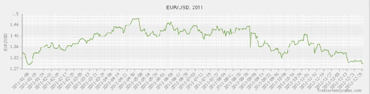
(17) consequences was Portugal, that despite compliance with the preconditions required, had a bad adaptation causing the sudden curb economic growth after a decade of large increases. Finally, fifth, all these countries achieved something I never could have achieved on their own, a strong currency against the outside, that even you can do against the US dollar. With this you get is a more credible currency because it is supported by 19 economies including countries with strong economies like Germany and France. This makes Europe more attractive for all types of investors. In addition, the euro gradually was getting stronger against the dollar. In Figure 8 below and then we can see the EUR / USD throughout 2011 where it reached a peak of 1.48 EUR / USD in the month of April. Figure 8. Growth of the euro against the dollar in 2011.. Source: datosmacro.com. Today, in 2015, the euro is losing much ground against the dollar due to a series of measures taken by the ECB trying to boost the European economy. Therefore, the ECB decided to devalue the currency trying to increase exports and reduce imports and thus obtaining a positive balance of payments. In Figure 9, attached below, is shown the evolution experienced by the euro in recent months. After a step descent to its lowest level in the month of March, its value has a gradually increasing, but without reaching the values of the past years.. 16.

(18) Figure 9. Growth of the euro against the dollar in 2015.. Source: datosmacro.com. After all, must be said that the aggregate between advantages and disadvantages is not yet clear. It is clear that some countries had more negative than positive consequences, while others were benefited from the beginning of the introduction of the euro in the territory.. 3.1. OUR MODEL Before starting this regression, in order to minimize the maximum margin of error, it is verified the possession of the data for each of the countries in all the interval years. Therefore there is an observation for each country and for each year. The dependent variable is the ratio of the current account to GDP. After evaluating different variables, this ratio is the most thigh for this study. A total of six explanatory variables were decided to be included. The real effective exchange rate (REER), the price of oil in real terms according to the data extracted from the IMF, the interest rate of 10-year bonds, the government deficit to GDP, the ratio of Net Foreign respect Assets of GDP and the openness of the economy from the rest of the world. With all these variables a regression will be performed to show how these variables affect the final balance of current accounts, that is, how they will affect the determination of the debit or credit balance. There are numerous works dealing with the same subject, but typically include many more variables. In our case a simpler and understandable model is chosen.. 17.

(19) As we have said before, the sample covers the data between 1970 and 2011. These countries that are chosen: Germany, Finland, Belgium, Spain, Greece and Ireland. To carry out this regression has been necessary to select those variables that conformed more to our ultimate goal. Most of the data we extracted from the database Milessi-Lane and Ferretti (2011). In this database we can be found a total of 28 variables with data on a total of 12 European countries. 6 of the variables used in the regression were extracted from this database, including 5 independent and one dependent. The independent variables obtained were the real effective exchange rate (REER), the interest rate of 10-year bonds (bond_yield), the public deficit to GDP (def_gdp), the net foreign assets ratio to GDP (nfa_gdp) and the degree of openness of economies (openness). The dependent variable used is the current account to GDP (ca_gdp). The other variable included in the regression is the price of oil in real terms (Oilprice), these data were obtained from the database of the International Monetary Fund. In this case, the variable is specific to each country data but annual world price. Table 2. Variables used in the model. Current Account / Gross Domestic Product (ca_gdp) Openness (openness) Real Effective Exchange Rate (reer) Deficit / Gross Domestic Product (def_gdp) Net Foreign Assets / Gross Domestic Product (nfa_gdp) Interest rate of 10-year bonds (bond_yield) Oil Price in Real Terms (oilprice). Dependent Independent Independent Independent Independent Independent Independent. Now each of the variables chosen for the work will be explained in greater depth: -. Current Account / Gross Domestic Product: It will be our dependent variable. This ratio is calculated as the ratio of public debt to gross domestic product of a country. This ratio shows the level of indebtedness of a country from the rest of the world. Some studies try to assess what percentage of debt would be a direct cause of insolvency of the state total. For example, in the work of Reinhart, Rogoff (2010), they came to the conclusion that this results in a higher ratio than 90% could lead to total bankruptcy, to be exact subject the country to a financial crisis. Later, other studies have reversed this theory based on the examples that gives us the same story, as may well be the case in the UK, which after the 18.

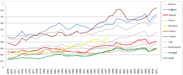
(20) two World Wars came to achieve a higher ratio to 250% without arrived to the bankruptcy of the state. In a period of about 20 years Britain was able to reduce this ratio to 50% approximate values. -. Openness: the degree of openness reflects the weight of the external sector (measured in terms of exports or imports of goods) on the gross domestic product adjusted for the size of the economy (home bias). By definition, the opening degree has positive values. A value less than one indicates that the economy is open to the world below, that is, exports are lower than they should be according to their weight in global GDP; a value greater than one indicates on openness to world markets, i.e., exports of the national economy to the world are higher than they should be about their economic weight.. In recent years, the level of openness of all European countries has been rising as we can well see in the chart below. This chart has been compiled from data from the database and Milessi-Ferreti Lane (2011). Countries which have different colours are countries included in the regression.. Figure 10. Evolution of openness in European countries.. 19.

(21) -. Real Effective Exchange Rate: is one of the main indicators of the external competitiveness of the national economy with another country or set of countries respectively. i.. When the REER increased, it implies a real appreciation of the national currency and a loss of external competitiveness of the national economy.. ii.. When the REER falls, it implies a real depreciation of the national currency and a gain of external competitiveness of the national economy.. Variations of the real effective exchange rate have great consequences on the economy, among them it is worth noting the following: i.. i. It will alter economic activity. It will affect aggregate due to disturbance on exports and imports demand.. ii.. It will alter the trade balance and the balance of goods and services. Provided that the "volume" effect outweighs the effect "price" (MarshallLerner), the real appreciation deteriorates the trade balance, while real depreciations improve the trade balance.. iii.. It affects the competitiveness of locally manufactured products compared to products manufactured abroad.. Figure 11 shows the evolution of the real effective exchange rate over the period 1994 - 2011. In this graph is shown the REER of Canada, Euro, Japan, USA and UK area. The data are drawn from the Federal Reserve Bank of St. Louis.. 20.

(22) Figure 11. Evolution of the real effective exchange rate.. Source: sefehaven.com. -. Public Deficit / GDP: the deficit also called tax and budget, shows that for a certain period of time, a State or Public Administration has committed a number greater than the income received spend, and therefore, to meet the payment of these expenses must borrow from abroad. The quantitative measurement of the public deficit is done through national accounts, which is what will give the most accurate measure of the deficit. Meanwhile, to measure the impact of the deficit on the economy is used to representing the deficit ratio to gross domestic product (GDP) will give the idea of transcendence presented.. 21.

(23) Figure 12. Accumulation of public deficits in European countries.. Source: BCE. -. Net foreign assets / GDP: We define net foreign assets as the difference between the amount of foreign assets in national property and national assets in foreign hands. Figure 13 shows the evolution of net foreign assets in the years 1999 to 2013. It found six European countries, Germany, Greece, Italy, Spain, Portugal and the UK. On numerous occasions these dividing GDP is used to compare with other economies data. As shown, two countries stand out for their totally opposite paths. On the one hand we find the case of Germany, which has managed to triple the total of foreign assets from almost zero to more than 1,500,000. Moreover is the case of Spain, which started from a situation with a negative balance but relatively close to zero. During these 13 years, Spain has achieved a negative balance of more than 1,000,000 million. As for the other countries included in this chart are more uniform trajectories, they all started in 1999 with negative balances very close to zero, over the years have been worsening his situation to stand at a near debt securities 500,000 million euros.. 22.

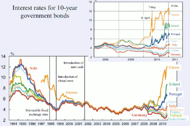
(24) Figure 13. Net foreign assets in some European countries.. Source: sefehaven,com. -. The interest rate of 10-year bonds: is calculated by adding the forecast of GDP growth plus inflation forecast of the economy. This estimate will only be reliable for countries benefiting from a good social and economic stability, otherwise could suffer major changes that move us away from reality. Although many forms of bonds available today in terms of its duration, 10-year bonds are chosen as a reference when investing in bonds and comparing investment in fixed income alternatives. Figure 14 shows the evolution of the interest rate of 10-year bonds of some European countries like Greece, Ireland, and Portugal, Spain, Italy, France, Belgium, Finland and the Netherlands. The data reflect the time period between 1994 and 2010. During this period, three major events are collected, such as the fixing of exchange rates in 1998, the virtual introduction of the euro and finally the introduction of the euro as Europe's common currency. In previous years to the fixing of exchange rates, changes in the real rate of the bonds were very distinct in different countries. The interest rate on a journey covering a nearly eight percentage points, reaching the lowest at 6% belonging to Germany, and the highest of 13.8% in Italy. Later, with the fixing of exchange rates he tended to converge, except for Greece, which was the only country with more disparate rates finally after the entry into force of the euro as a common European currency, Greece managed to achieve the rates of other countries and thus converge. 23.

(25) This stability was maintained until the outbreak of the crisis in 2007. Since then interest rate of 10-year bonds again diverge. Greece was again the farthest country from the average, reaching almost 13 percentage points in late 2010. Other countries that most increased their rates were Ireland, Portugal, Spain and Italy, coinciding with the most affected countries by the crisis. On the opposite side we have Germany and Finland, which unlike the other countries managed to reduce its rate near 2% coinciding again with the countries least affected by the financial crisis. Figure 14. Interest rate developments of ten-year bonds in some European countries.. -. Price in real terms oil: the price of oil has fluctuated in recent years with strong implications for the global economy. An increase in oil prices leads to an increase in inflation and therefore a lower demand of the different economic agents. Thus we see that there is a direct relationship between changes in oil prices and the consequent change in demand, it is much more difficult to explain the ways in which these price changes affect supply.. 24.

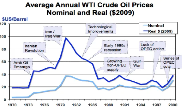
(26) Graphic 15 shows the evolution of oil prices in both real and nominal terms, they are also featured those events occurred during the period have caused disturbances. This graph covers the period of 1970-2000. Roughly speaking matching between the evolution of real and nominal prices is observed; throughout the entire period real prices have been much higher, until at the end of 2000 almost completely converged. These two major events impacted significantly on the price of oil. First, in mid1973 the well-known oil crisis appeared, caused by the decision of the Organization of Arab Petroleum Exporting Countries (OPEC) members of the Persian Gulf. Their decision was not to export more oil to countries that supported Israel during the war. This affected squarely the United States and its Western European allies. Another of the events that had the greatest impact was the Iran-Iraq war that took place between 1980 and 1988, which had a high social and economic cost. During the military conflict and subsequent same time, oil exports were disrupted, so it was a high rise in the real price of oil. As shown in the graph, this price rise started between 1978 and 1980, from about $ 50 a barrel to its maximum of $ 100 in 1980. This large increase had a major impact on all economies that had great energy dependence.. Figure 15. Evolution of oil prices over the last 30 years.. 25.

(27) In Figure 16 is shown in greater detail the real price of oil over the past fifteen years. Until the end of 2007 the price of oil was rising in a gradual way, until early 2008 due to the outbreak of the crisis the price increase disproportionately and in a relatively short time. In January 2007 the price of oil per barrel was around $ 100.52 while its peak in July 2008 reached $ 249.66, this being the highest price in history. After the peak, a sudden drop of over $ 150 per barrel experienced, reaching its minimum in December of that year when the oil price stood at $ 77.71. After these strong fluctuations occurred a time of stability in the price of oil it remained around $ 200, until mid-2014 again experienced a big drop reaching its minimum in January of 2015 when it reached 89, $ 15 per barrel. Figure 16. Real price of oil over the last 15 years.. Source: BCE. 26.

(28) 4. REGRESISON. 4.1. RESULTS OBTAINED IN GENERAL REGRESSION After performing the Hausman test and resolve to perform regression using the fixed effects model, we decided to carry out the estimation of the variables affecting the current account in two different sections. In the first section, we performed a joint regression with all the data at our disposal using a panel approach. There is included the observations from six European countries, Belgium, Finland, Spain, Greece and Ireland. For each country we have a time series between 1970 and 2011, and six explanatory variables: . Net Foreign Assets. . Openness. . Real Effective Exchange Rate. . Public deficit / GDP. . Interest of 10-year bonds. . Oil price in real term. In Table 3 attached below we can see the results obtained in the panel regression. We have used the method from the general to the particular. From an initial regression in which all the explanatory variables included, we have gradually eliminating those variables that had a lower level of significance.. 27.

(29) Table 3. FE panel robust regression. EXPLANATORY VARIABLES. Dependent Variable : Current Account (1) (4) Net Foreign Assets / GDP 0.256 0.258*** (1.18) (5.21) Openness 0.399* 0.294* (1.84) (1.81) Real Effective Exchange 0.095 (0.87) Public Deficit / GDP -0.105 -0.096 (-1.61) (-0.47) 0.000 Real interest rate of 10year bonds (0.00) Oil Price 0.506 (1.33) Constant 23.853 58.743*** (0.60) (5.99) The numbers between * α = 0.10 ** α = 0.05 *** α = 0.01 parentheses are the t-student. In the first column of the table we observe the name of each of the explanatory variables used in the regression. The second column is the output obtained in the regression that included all variables. Finally in the third column we find the regression in which we have excluded those less significant variables. After keeping only those explanatory variables with greater significance we have obtained two significant variables: . Net Foreign Assets / GDP: as we may well observe this is the variable with greater significance, as it is significant even for α = 0.01. It is expected that this variable had a positive sign because in the calculation of the current account of the different countries, net foreign assets are included with a positive sign. Indeed, the sign obtained is positive. According to data obtained an increase of 1% in net foreign assets an increase in the value that would affect the current account of a 0.258%.. . Openness: in the case of this variable we also note that is significant but only for α = 0.10. Would be expected that had positive sign, because a greater degree of openness implies greater freedom in the movement of capital and goods and services. Indeed the sign obtained in this regression is positive in line with expectations. According to the data shown in the table an increase of 28.

(30) 1% of the openness of the economy would produce an increase in the current account of the country of 0.294%. 4.2.. RESULTS OBTAINED IN THE TIME SERIES – APPROACH. After the panel estimation, we turn to individual analysis of each country, in which the same independent variables and the dependent variable itself are maintained. Again we used the method from the general to the particular, phasing out the variables with lower degree of significance to maintain only three explanatory variables for each country. In Table 4 attached below we can see the results. The first column shows all the explanatory variables used in the regression, and then we used two columns for each country, in the first initial regression is shown with all variables and in the adjacent column is shown the regression using only the three variables with greater significance.. 29.

(31) Constant. Real interest rate of 10year bonds Oil Price. Public Deficit / GDP. Real Effective Exchange. Openness. Net Foreign Assets / GDP. EXPLANATORY VARIABLES. Germany (1) 0.622*** (5.30) 0.327* (1.73) 0.246* (1.83) 0.051 (0.39) 0.191 (-1.06) 0.031 (0.26) -2.791 (-0.35) -7.297 (-1.54). Germany (4) 0.607*** (5.43) 0.471*** (3.54) 0.221* (1.71). Dependent Variable : Current Account Belgium (1) Belgium (4) Finland (1) Finland (4) Spain (1) 0.059 -0.015 -0.254 (0.26) (-0.09) (-0.55) -0.324* -0.311** 0.163 0.195 0.676 (-1.85) (-2.17) (0.88) (1.27) (1.06) 0.133 0.146** 0.117 -0.269 (1.37) (2.06) (0.60) (-1.40) 0.005 0.097 -0.414* (-0.06) (0.57) (-1.87) 0.321 0.284 0.551 0.419 -0.381 (1.22) (1.32) (1.47) (1.39) (-1.20) 0.027 0.302* 0.358*** 0.204 (0.36) (1.89) (2.51) (1.32) 9.558 12.018 7.931 10.922** 24.729*** (0.83) (1.63) (1.01) (2.17) (3.67) 0.176 (1.21) 28.231*** (5.13). -0.359** (-2.13) -0.265 (-1.60). Spain (4). Greece (1) 0.105 (0.44) 0.547*** (2.78) -0.336** (-2.00) -0.049 (0.32) 0.189 (0.91) 0.173 (1.36) 7.638 (1.29). Greece (4) Ireland (1) Ireland (4) 0.444*** 0.407*** (2.40) (2.80) 0.699*** -0.116 -0.307 (5.21) (-0.47) (-1.60) -0.319*** -0.153 (-2.44) (-0.80) -0.089 (-0.55) 0.432* 0.473*** (1.70) (2.33) 0.142 -0.058 (1.24) (-0.35) 8.017* 11.863 11.126*** (1.65) (1.18) (2.82). Table 4. Individual regressions for each country.. 30.

(32) We will discuss the data of individual countries to finally make a comparison between them. . Germany: once we have eliminated all variables with lower levels of significance we have obtained a final regression including Net Foreign Assets / GDP, Openness and Real Effective Exchange Rate. All are significant at least for α = 0.10. -. Net Foreign Assets / GDP: in this case a positive sign as expected is obtained. A 1% increase in NFA / gdp would represent an increase in Germany's current account of a 0.607%.. -. Openness: again the expected positive sign for this variable is met. An increase of 1% would affect openness in the current account an increase of a 0.471%.. -. REER: Before the arrival of the euro as a common currency, the German mark had considered a strong currency, so that after the change is depreciated over the previous period. This depreciation has caused an increase in exports and decreased imports, which impacts positively on its current account. Would expect in this case that the REER had a positive sign indeed this is true. A 1% increase in the REER would cause an increase in the German current account of a 0.221%. This variable is only significant for α = 0.10.. . Belgium: again we removed those explanatory variables lower explanatory power and those included in the final specification are Openness, the Real Effective Exchange Rate and the Real interest rate of 10-year bonds. Of these three are only significant Openness and REER. -. Openness: in this case the variable does not show the sign would be expected, because a negative is obtained. In this case, a 1% increase in opening degree would produce a decrease in the Belgian current account of a 0.311%.. -. REER: In Belgium, has happened something like in Germany, an increase in exports could have positive effects on current account, so would expect a positive sign that is effectively obtained. A 1% increases in the REER produce an increase of the current account in Belgium of a 0.146%.. 31.

(33) . Finland: again after removing the variables with lower degree of significance, we maintained only three, in this case are Openness, Real interest rate of 10-year bonds and Oil price. Of these three only reaches a level of significance of at least the variable α = 0.10 Oil Price. -. Oil Price: in this case we would expect Oil Price had negative sign, but not, so in the case of Finland presents positive sign. A 1% increase in oil prices would represent an increase of Finnish current account of a 0.302%.. . Spain: in this case the remaining variables in the regression ordered according to their level of significance are the REER, Public deficit / GDP and Oil Price. Of these three, only REER is significant at least to a level of α = 0.10. -. REER: Spain before the introduction of the common currency had a weak currency, which has meant that with the euro as a common currency have been their exports more expensive and thus these have decreased while imports become cheaper, so this will have a negative impact on the current account.. . Greece: in this case the variables with the highest significance are Openness, REER and Oil Price. -. Openness: one would expect that this variable had a positive sign indeed this is true. A 1% increase in the degree of opening Greek will produce an increase of 0.699% of the current account.. -. REER: the Greek situation is very similar than the Spanish one, before the common currency had a coin considered weak, so after the introduction of Euro exports decreased due to higher prices and increased imports, again we wait for negative sign. Effectively we obtain negative regression. An increase of of 1% will cause a decrease REER Greek current account of a 0.319%.. . Ireland: the most significant variables in this country are Net Foreign Assets, Openness and Real interest rate of 10-year bonds. -. Net Foreign Assets: as expected we obtain a positive sign, as an increase in assets will have a positive effect on the value of the current account. An increase of 1% of the Net Foreign Assets cause an increase in the current account of a 0.407%.. -. Real interest rate of 10-year bonds: one would expect a positive sign. A 1% increase in the real interest rate of 10-year bonds will. 32.

(34) cause an increase in the current account of a 0.473% of Irish current account. Once analysed all significant variables from the six countries we will make a comparison separating countries into two groups. In the first group are the countries that have historically had a positive balance most of the years analysed, which will be Germany, Belgium and Finland in this case. In the second group are those countries whose balance has been most negative years. In Table 5 is shown a brief summary to make it easier to visualize. Table 5. Summary of significant variables for each country.. nfa_gdp openness reer def_gdp bond_yield oilprice. Germany x x x. Belgium. Finland. x x. Spain. Greece. x. x x. Ireland x. x x. As we can observe in the first group none of the explanatory variables included it is significant for the three countries at once. But we found similarities between the regressions of Germany and Belgium, which agree on the degree of openness and in the REER. Finland only has a significant variable which does not coincide with Germany and Belgium. In the second group also we found no explanatory variable that is significant for the three countries at once. Spain and Greece coincide in the case of the REER, while Ireland has two explanatory variables which do not match any of those obtained in the two other countries. By looking at all countries at the same time we could say that the most significant explanatory variable would be the REER, which is present in four of the six countries. Common less would be the interest rate of ten-year bonds and the price of oil. 4.3. SPECIFICATION TESTS 4.3.1. Lack of correlation To verify that there is no correlation among residues in our regressions we decided to perform a test using Stata. In Table 6 attached below we observe the degree of correlation of the residuals of each of the countries. We understand that a value of 1 or 33.

(35) closer implies a high level of correlation, while a value closer to zero implies a lesser degree of correlation. We see that in the case of Germany, Belgium and Greece there is a high level of correlation of the residues regarding to the current account. In the case of Spain a lower correlation is obtained, which barely reaches 0.5. Table 6. Correlation test.. Correlation. Germany 0.809. CORRELATION Finland Belgium 0.682 0.833. Spain 0.502. Greece 0.816. Ireland 0.606. 4.3.2. Lack of heteroskedasticity We see that there isn't heteroskedasticity in our regressions. For this we have made the White’s test. In this case the null hypothesis is that there exists homoskedasticity. Table 7 attached below shows the obtained results for each country. As we can see, in all countries except Ireland we must reject the null hypothesis assuming no homoskedasticity. Because heterokedasticity occurs we must perform regressions in which the indicators must be robust to thereby solve the problem of heteroskedasticity. Ireland need not apply robust indicators as its own data show the presence of homoskedasticity. The results obtained by using robust indicators will be presented in Table 4 that we can see further.. Table 7. White test.. Prob>chi(2). Germany 0.174. WHITE TEST Finland Belgium 0.403 0.386. Spain 0.222. Greece 0.177. Ireland 0.596. 4.3.3. Stationarity To verify that there is no remaining non-stationarity in our data we have decided to perform the Dickey-Fuller test (DFA test) to the residuals of each of the regressions. It is a test of non- stationarity because the null hypothesis is the presence of a unit root in the data generating process (in this case in the residuals) of the series analysed. In Table 8 we can see the obtained results.. 34.

(36) Table 8. DFA test.. t-Statistic. Germany -1.959. Finland -2.392. ADF TEST Belgium -2.236. Spain -3.627*. Greece -1.979. Ireland -2.309. The null hypothesis posed by DFA test implies that there is cointegration. The only case where there is clear evidence of cointegration is Spain. This test is essential to continue with the analysis as, otherwise, the results may be spurious.. 35.

(37) 5. CONCLUSION Our initial aim was finding some of the variables that would help us to explain why some countries had achieved during the last 41 years the current account surplus while others obtained deficits. After analysing all the data we can say that we have found significant differences between selected countries. Significant for each explanatory variables are different. Germany's current account is determined by the Net Foreign Assets, the degree of openness of the economy and in REER. The CA of Belgium for the openness and REER. Finland CA oil prices. Spain CA only by REER. In the case of Greece by the degree of openness and the REER. Finally, Ireland by Net Foreign Assets and the interest rate of ten-year bonds. We obtained cointegration only in Spain case. We should continue working in this issue and deeper. This would require improving the estimation and use other techniques that are not included in our work. We can see that in the panel it is satisfactory results which urge us to continue working in the paper. We have found considerable heterogeneity between countries, despite belonging to a single economic area. This heterogeneity is the result of various macroeconomic policies adopted by each country, which give a different weight to each of the variables included in the model. In conclusion, we can say that we have achieved the results we expected, which show that during the time period between 1970 and 2011 determining the balance of the current account included in the model are different for each of the countries analysed. This diversity in the explanatory variables determines if a country gets deficit or current account surplus.. 36.

(38) 6. REFERENCES (bAg): Blog de economía de la AldEa Global, (2011). Evolución del tipo de cambio efectivo real de los países industrializados y de los principales países emergentes, 1994-2011. [online] Available at: http://blogaldeaglobal.com/2011/11/28/evolucion-deltipo-de-cambio-efectivo-real-de-los-paises-industrializados-y-de-los-principales-paisesemergentes-1994-2011/ [Accessed 2 Jun. 2015]. Aizenman, J., Chinn, M. and Ito, H. (2013). The Impossible Trinity• Hypothesis in an Era of Global Imbalances: Measurement and Testing. Review of International Economics, 21(3), pp.447-458. Algieri, B. and Bracke, T. (2009). Patterns of Current Account Adjustment : Insights from Past Experience. Open Economies Review, 22(3), pp.401-425. Barthelemy, J. and Cleaud, G. (n.d.). Global Imbalances and Imported Disinflation in the Euro Area. SSRN Journal. Baum, C., Schaffer, M. and Stillman, S. (2011). USING STATA FOR APPLIED RESEARCH: REVIEWING ITS CAPABILITIES. Journal of Economic Surveys, 25(2), pp.380-394. Berger, H. and Nitsch, V. (2014). Wearing corset, losing shape: The euro's effect on trade imbalances. Journal of Policy Modeling, 36(1), pp.136-155. Bueno, J. (2015). La liberalizacion del mercado de capitales en Europa. [online] EL PAÍS. Available at: http://elpais.com/diario/1986/11/10/economia/531961202_850215.html [Accessed 14 Jun. 2015]. Catão, L. and Milesi-Ferretti, G. (2013). External Liabilities and Crises. IMF Working Papers, 13(113), p.1. Chinn, M. and Prasad, E. (2003). Medium-term determinants of current accounts in industrial and developing countries: an empirical exploration. Journal of International Economics, 59(1), pp.47-76. Corden, W. (2007). Those Current Account Imbalances: A Sceptical View. The World Economy, 30(3), pp.363-382. Cuánticos, C. (2011). Saca la basura y no te olvides de las hipotecas. [online] Cuentos Cuánticos. Available at: http://cuentos-cuanticos.com/2011/11/20/saca-la-basura37.

(39) y-no-te-olvides-de-las-hipotecas/ [Accessed 18 May 2015]. Datos.bancomundial.org, (2015). Saldo en cuenta corriente (balanza de pagos, US$ a precios actuales) | Datos | Tabla. [online] Available at: http://datos.bancomundial.org/indicador/BN.CAB.XOKA.CD [Accessed 19 May 2015]. datosmacro.com, (2015). Comparar economáa países: Irlanda vs España 2015. [online] Available at: http://www.datosmacro.com/paises/comparar/irlanda/espana [Accessed 4 May 2015]. datosmacro.com, (2015). Deuda Pública de Estados Unidos 2015. [online] Available at: http://www.datosmacro.com/deuda/usa [Accessed 11 May 2015]. Definición ABC, (2015). Definición de Déficit publico. [online] Available at: http://www.definicionabc.com/economia/deficit-publico.php [Accessed 11 May 2015]. Eleconomista.es, (2015). Francia, China, Benelux y Alemania, los principales acreedores de la deuda española - elEconomista.es. [online] Available at: http://www.eleconomista.es/economia/noticias/2213161/06/10/Francia-ChinaBenelux-y-Alemania-los-principales-acreedores-de-la-deudaespanola.html#.Kku8e1F38XFMskf [Accessed 14 May 2015]. Elsentidodelavida.com, (2015). La saga de Dashiell: Los quince mayores acreedores de Estados Unidos. [online] Available at: http://www.elsentidodelavida.com/2012/02/los-quince-mayores-acreedoresde.html [Accessed 9 May 2015]. Europarl.europa.eu, (2015). Libre circulación de capitales. [online] Available at: http://www.europarl.europa.eu/aboutparliament/es/displayFtu.html?ftuId=FTU_3.1 .6.html [Accessed 7 May 2015]. Expansion.com, (2015). El inversor consciente - La relación entre deuda, déficit y PIB.. [online] Available at: http://www.expansion.com/blogs/el-inversorconsciente/2012/11/01/la-relacion-entre-deuda-deficit-y-pib.html [Accessed 1 Jun. 2015]. Freecurrencyrates.com, (2015). Historia del tipo de cambio en el año 2011 de Euro (EUR) y Dólar estadounidense (USD). [online] Available at: http://www.freecurrencyrates.com/es/exchange-rate-history/EUR-USD/2011 38.

(40) [Accessed 14 Jun. 2015]. Hamilton, L. (2006). Statistics with Stata. Belmont, CA: Thomson/BrooksCole. Indexmundi.com, (2015). Indice de precios del petróleo crudo - Precio Mensual Precios de Mercancías. [online] Available at: http://www.indexmundi.com/es/precios-de-mercado/?mercancia=indice-deprecios-del-petroleo-crudo&meses=180 [Accessed 7 May 2015]. Kang, J. and Shambaugh, J. (2014). Progress Towards External Adjustment in the Euro Area Periphery and the Baltics. IMF Working Papers, 14(131), p.1. Lane, P. and Milesi-Ferretti, G. (2014). Global Imbalances and External Adjustment after the Crisis. IMF Working Papers, 14(151), p.1. Libertaddigital.com, (2015). Los españoles elevan su ahorro para protegerse del paro y del Gobierno - Libertad Digital. [online] Available at: http://www.libertaddigital.com/economia/los-espanoles-disparan-el-ahorro-porquetemen-al-paro-y-al-gobierno-1276374629/ [Accessed 3 May 2015]. Mars, A. (2014). España es el segundo país con mayor deuda externa tras Estados Unidos. [online] EL PAÍS. Available at: http://economia.elpais.com/economia/2014/09/30/actualidad/1412081072_163414 .html [Accessed 13 Jun. 2015]. Mars, A. (2014). España es el segundo país con mayor deuda externa tras Estados Unidos. [online] EL PAÍS. Available at: http://economia.elpais.com/economia/2014/09/30/actualidad/1412081072_163414 .html [Accessed 14 Jun. 2015]. Mars, A. (2014). España pagará casi 100 millones diarios por los intereses de su deuda. [online] EL PAÍS. Available at: http://economia.elpais.com/economia/2014/09/30/actualidad/1412067224_399518 .html [Accessed 10 May 2015]. Observatorioabaco.es, (2015). Grado de apertura, conexión e integración - ABACO. [online] Available at: http://www.observatorioabaco.es/post_observatorio/gradode-apertura-conexion-e-integracion-3 [Accessed 2 Jun. 2015]. País, E. (2015). Liberalización del mercado de capitales. [online] EL PAÍS. Available at: http://elpais.com/diario/1986/10/20/opinion/530146808_850215.html [Accessed. 39.

(41) 18 May 2015]. Reinhart, C. and Rogoff, K. (2010). Growth in a Time of Debt. American Economic Review, 100(2), pp.573-578. Reinhart, C. and Rogoff, K. (2010). Growth in a Time of Debt. S.L., U. (2015). Tipo de cambio real. [online] Expansion.com. Available at: http://www.expansion.com/diccionario-economico/tipo-de-cambio-real.html [Accessed 16 Apr. 2015]. Safehaven.com, (2015). Europe Throws a Hail Mary Pass | John Mauldin | Safehaven.com. [online] Available at: http://www.safehaven.com/article/16808/europe-throws-a-hail-mary-pass [Accessed 6 Apr. 2015]. Schoder, C., Proaño, C. and Semmler, W. (2012). ARE THE CURRENT ACCOUNT IMBALANCES BETWEEN EMU COUNTRIES SUSTAINABLE? EVIDENCE FROM PARAMETRIC AND NON-PARAMETRIC TESTS. Journal of Applied Econometrics, 28(7), pp.1179-1204. Tedxdu.com, (2014). Currency Options Market | Tedxdu Ideas worth spreading. [online] Available at: http://www.tedxdu.com/tag/currency-options-market/ [Accessed 8 May 2015]. Transportationfortomorrow.com, (2015). National Surface Transportation Policy and Revenue Commission. [online] Available at: http://transportationfortomorrow.com/final_report/volume_3_html/technical_issues _papers/paper42cc.htm?name=4c_06 [Accessed 14 Jun. 2015].. 40.

(42)