Reconstruction problems for LGT networks

Texto completo

(1) . . DOCTORAL THESIS 2016 . . . RECONSTRUCTION PROBLEMS FOR LGT NETWORKS . . Joan Carles Pons Mayol .

(2)

(3) DOCTORAL THESIS 2016 Doctoral Programme of Mathematics. RECONSTRUCTION PROBLEMS FOR LGT NETWORKS. Joan Carles Pons Mayol. Thesis Supervisor: Dr. Gabriel Cardona Juanals Doctor by the Universitat de les Illes Balears.

(4)

(5) Statement of Authorship This thesis has been submitted to the Escola de Doctorat, Universitat de les Illes Balears, in fulfilment of the requirements for the degree of Doctor en Matemàtiques. I hereby declare that, except where specific reference is made to the work of others, the content of this dissertation is entirely my own work, describes my own research and has not been submitted in whole or in part for consideration for any other degree or qualification in this, or any other university.. Joan Carles Pons Mayol Palma, September 2016. Funding The work reported in this thesis was supported by Ministerio de Ciencia e Innovación through grants Grafos en biologı́a computacional (MTM2009 07165), Aplicaciones bioinformáticas en filogenética, metagenómica, biologı́a de sistemas y genómica del cáncer (DPI2015-67082-P), Creación de una red temática en computación biomolecular y celular (TIN2008-04487-E/TIN) and Renovación y nuevas actividades de la red temática en computación biomelecular y biocelular (TIN2011-15874-E) and Obra Social “La Caixa” through Programa Pont “La Caixa” per a grups de recerca de la UIB.. i.

(6) ii.

(7) Supervisor’s Agreement I, Gabriel Cardona, Ph.D. in Mathematics and Associate Professor at the Department of Mathematics and Computer Science, Universitat de les Illes Balears. ATTEST THAT. this dissertation, titled Reconstruction Problems for LGT Networks and submitted by Joan Carles Pons Mayol for obtaining the degree of Doctor en Matemàtiques, was carried out under my supervision and contains enough contributions to be considered as a doctoral thesis.. Dr. Gabriel Cardona Palma, September 2016. iii.

(8) iv.

(9) Abstract Phylogenetics is the study of evolutionary history and relationships among species, and in particular, its reconstruction from biological data. It plays an important role in understanding biology because it allows to stablish the relationships between organisms. Based on Darwin’s theory, which states that all species have evolved from a common ancestor, evolutionary histories have been represented using trees. However, when non-vertical evolutionary events such as hybridizations, recombinations and lateral transfer of genes occur, the use of phylogenetic networks is indeed more appropriate than trees in order to model those reticulate evolutionary histories. The main motivation of this thesis is to develop a new model for phylogenetic networks modelling evolutionary histories with lateral gene transfers, as well as computational methods and algorithms for their reconstruction. The new model we propose, which we call LGT networks, captures the asymmetry of lateral gene transfer events. The model is based on considering a principal tree that represents the main line of evolution of the considered species, and a set of arcs modelling lateral transfer events. Our LGT networks generalizes some other existent models which were designed for a similar purpose. We solve the well-known phylogenetic network reconstruction problem for the abovementioned LGT networks from induced sets of trees and trinets. Both cases require some topological constraints to be imposed in order to obtain unicity of solutions, which is lost when considering generic LGT networks. We reconstruct such networks from a set of trees formed by a principal tree and a set of secondary subtrees, being each of these secondary subtrees associated to a specific secondary arc. To do this, we propose a polynomial algorithm, which we applied to real biological data sets in order to predict or discover lateral transfer events. We also study the reconstruction problem from a set of “basic” LGT networks on three leaves and with only one secondary arc. We call such networks tri-lgt-nets, which are similar to the well-known trinets. With this, we contribute to extend the set of possible phylogenetic networks that can be recovered using the previous substructures. Finally, we extend the framework for the reconciliation problem between gene trees and species trees using LGT networks as the species phylogeny. In order to set up the evolutionary scenario, we allow transfer events via secondary arcs of the network only, as well as duplications and losses. For this model, we present fast computational algorithms addressed to obtain the most parsimonious reconciliation between a gene tree and an LGT network.. v.

(10) vi.

(11) Resum La filogenètica és l’estudi de les històries evolutives i les relacions entre espècies, i en particular la seva reconstrucció a partir de dades biològiques. Aquesta juga un paper important en la comprensió de la biologia, ja que permet determinar les relacions de parentiu entre organismes. Basant-se en la teoria de Darwin, la qual defensa que totes les espècies han evolucionat d’un ancestre comú, les històries evolutives s’han representat emprant arbres. No obstant això, quan ocorren processos evolutius no verticals tals com hibridacions, recombinacions i transferències laterals de gens, l’ús de xarxes filogenètiques és, certament, més apropiat que l’ús d’arbres per a modelar aquestes històries evolutives reticulars. La principal motivació d’aquesta tesi és desenvolupar un nou model per a xarxes filogenètiques que modelen històries evolutives amb transferències laterals de gens, aixı́ com mètodes computacionals i algorismes per a la seva reconstrucció. El nou model que proposem, i que anomenem xarxes LGT, captura l’asimetria de les transferències laterals de gens. El model es basa en considerar un arbre principal, representant la lı́nia principal d’evolució de les espècies considerades, i un conjunt d’arcs modelant les transferències laterals de gens. Les nostres xarxes LGT generalitzen altres models ja existents que foren dissenyats amb un propòsit similar. Resolem també el problema ben conegut de reconstrucció de xarxes filogenètiques per a les esmentades xarxes LGT a partir de conjunts induı̈ts d’arbres i de trinets. Ambdós casos requereixen que s’hi imposin algunes restriccions topològiques per obtenir unicitat de solucions, que es perd considerant xarxes LGT genèriques. Reconstruı̈m aquestes xarxes a partir d’un conjunt d’arbres format per un arbre principal i un conjunt d’arbres secundaris. Cadascun d’aquests últims està associat a un arc secundari especı́fic. Per fer-ho, proposem un algorisme polinòmic que apliquem a dades biològiques reals per a predir o descobrir processos de transferència lateral de gens. També estudiem el problema de reconstrucció a partir d’un conjunt de xarxes LGT “bàsiques” de només tres fulles i un sol arc secundari. Anomenarem a aquestes xarxes, xarxes tri-lgt-nets que serien similars a les conegudes trinets. Amb això, contribuı̈m a estendre el conjunt de xarxes filogenètiques que poden ser reconstruı̈des emprant les subestructures prèvies. Finalment, estenem el marc del problema de reconciliació entre arbres de gens i arbres d’espècies emprant les xarxes LGT com a filogènia d’espècies. Per establir l’escenari evolutiu, permetem les transferències laterals de gens, només a través dels arcs secundaris de la xarxa, aixı́ com també duplicacions i pèrdues. Per això, presentem algorismes computacionals ràpids adreçats a obtenir la reconciliació més parsimoniosa entre un arbre de gens i una xarxa LGT.. vii.

(12) viii.

(13) Resumen La filogenética es el estudio de las historias evolutivas y las relaciones entre especies, y en particular de su reconstrucción a partir de datos biológicos. Esta juega un papel importante en la comprensión de la biologı́a puesto que permite establecer las relaciones de parentesco entre organismos. Bajo la teorı́a de Darwin, que defiende la procedencia de todas las especies de un ancestro común, las historias evolutivas han sido representadas usando árboles. No obstante, cuando ocurren procesos evolutivos no verticales cómo hibridaciones, recombinaciones o transferencias laterales de genes, el uso de redes filogenéticas es, ciertamente, más apropiado que el uso de árboles para modelar estas historias evolutivas reticulares. La principal motivación de esta tesis es desarrollar un nuevo modelo para redes filogenéticas que modelan historias evolutivas con transferencia lateral de genes, además de métodos computacionales y algoritmos para su reconstrucción. El nuevo modelo que proponemos, que llamamos redes LGT, captura la asimetrı́a de las transferencias laterales de genes. El modelo se basa en considerar un árbol principal representando la lı́nea principal de evolución de las especies consideradas y un conjunto de arcos modelando las transferencias laterales de genes. Nuestras redes LGT generalizan otros modelos ya existentes que fueron diseñados con un propósito similar. Resolvemos el conocido problema de reconstrucción de redes filogenéticas para las mencionadas redes LGT a partir de conjuntos inducidos de árboles y trinets. En ambos casos se requiere la imposición de restricciones topológicas para obtener unicidad en las soluciones, ya que esta se pierde cuando consideramos redes LGT genéricas. Reconstruimos estas redes a partir de un conjunto de árboles formado por un árbol principal y un conjunto de árboles secundarios. Cada uno de estos últimos está asociado a un arco secundario especı́fico. Para hacerlo, proponemos un algoritmo polinomial que aplicamos sobre datos biológicos reales para predecir o descubrir procesos de transferencia lateral de genes. También estudiamos el problema de reconstrucción a partir de un conjunto de redes LGT “básicas” de unicamente tres hojas y un sólo arco secundario. Llamamos a estas últimas redes tri-lgt-nets, similarares a las conocidas como trinets. Con esto, contribuimos a extender el conjunto de posibles redes filogenéticas que se pueden reconstruir usando estas subestructuras. Finalmente, extendemos el marco del problema de reconciliación entre árboles de genes y árboles de especies usando las redes LGT cómo filogenia de especies. Con el fin de establecer el escenario de evolución permitimos transferencias laterales de genes, sólo a través de los arcos secundarios de la red, ası́ como también duplicaciones y pérdidas. Para esto, presentamos algoritmos computacionales rápidos dirigidos a obtener la reconciliación más parsimoniosa entre un árbol de genes y una red LGT de especies.. ix.

(14) x.

(15) Agraı̈ments Arribat aquest moment i després del recorregut que m’ha portat fins aquı́, no vull deixar passar l’oportunitat d’expressar el meu agraı̈ment: • Al meu director, Biel Cardona, pel seu suport i seguiment durant la meva carrera universitària des dels meus inicis i fins al dia d’avui. Sense ell, aquest treball de recerca no hauria estat possible i, el meu interès per l’àlgebra, tampoc. • Al grup de Biologia Computacional i Bioinformàtica (BIOCOM) de la Universitat de les Illes Balears (UIB), per contribuir a la meva formació, especialment a Cesc Rosselló com a director del grup. • Al Departament de Matemàtiques i Informàtica de la UIB i en representació seva a Ricardo Alberich, director del mateix durant aquest treball de tesi. • A na Cati Vich, per tot (hi ha massa coses per anomenar-les totes). • A en Joan Duran i na NN Vich; cadascun en sap els motius particulars però, gràcies per ser-hi, recolzar-me i ajudar-me en tot moment. • Als amics d’Algaida i altres companys del departament de la UIB, pel seu interès a seguir i conèixer el meu camı́. • À Céline Scornavacca pour le traitement et l’aide qu’elle m’a donné, dans et hors l’université pendant mon séjour de recherche à Institut des Sciences de l’Evolution, Université Montpellier II. • To Krzysztof Bartoszek, Marta Casanellas and Jesús Fernández to open the doors and for the help they have provided me with during my visits in Uppsala University and Departament de Matemàtica Aplicada I, Universitat Politècnica de Catalunya, respectively. • Als meus pares, la meva germana i als meus avis, per la seva ajuda i la força que m’han transmès. • A en Miquel Amengual, al que li dec la meva passió per les matemàtiques des de ben jove.. xi.

(16) xii.

(17) Contents. Introduction. 1. 1 Preliminaries. 7. 1.1. Graphs . . . . . . . . . . . . . . . . . . . . . . . . . . . . . . . . . . . . . . .. 7. 1.2. Some biological concepts . . . . . . . . . . . . . . . . . . . . . . . . . . . . .. 9. 1.3. Trees and networks in phylogenetics . . . . . . . . . . . . . . . . . . . . . . 11. 1.4. Newick notation for trees and networks. 1.5. Decomposition of trees and networks . . . . . . . . . . . . . . . . . . . . . . 14. 1.6. Classification of phylogenetic networks . . . . . . . . . . . . . . . . . . . . . 16. 1.7. Topological restrictions . . . . . . . . . . . . . . . . . . . . . . . . . . . . . . 17. 1.8. Metrics on phylogenetic networks . . . . . . . . . . . . . . . . . . . . . . . . 22. 1.9. Phylogenetic networks reconstruction . . . . . . . . . . . . . . . . . . . . . . 26. . . . . . . . . . . . . . . . . . . . . 12. 1.10 Reconciliation between gene trees and species trees . . . . . . . . . . . . . . 28 2 LGT networks. 33. 2.1. Introduction . . . . . . . . . . . . . . . . . . . . . . . . . . . . . . . . . . . . 33. 2.2. LGT networks. 2.3. LGT networks generalize species graphs . . . . . . . . . . . . . . . . . . . . 37. 2.4. Other models for LGT events . . . . . . . . . . . . . . . . . . . . . . . . . . 37. 2.5. An extension of Robinson-Foulds metric for LGT networks. . . . . . . . . . . . . . . . . . . . . . . . . . . . . . . . . . . 34. . . . . . . . . . 39. 3 A reconstruction problem for LGT networks based on trees. 43. 3.1. Introduction . . . . . . . . . . . . . . . . . . . . . . . . . . . . . . . . . . . . 43. 3.2. Secondary and reduced subtrees . . . . . . . . . . . . . . . . . . . . . . . . . 44. 3.3. Subtree prune and regraft on LGT networks . . . . . . . . . . . . . . . . . . 45 xiii.

(18) CONTENTS 3.4. LGT network reconstruction problem . . . . . . . . . . . . . . . . . . . . . . 46. 3.5. Restricted LGT networks . . . . . . . . . . . . . . . . . . . . . . . . . . . . 48. 3.6. Computational experiments . . . . . . . . . . . . . . . . . . . . . . . . . . . 62. 3.7. Some technical proofs . . . . . . . . . . . . . . . . . . . . . . . . . . . . . . 66. 4 A reconstruction problem for LGT networks based on tri-lgt-nets. 77. 4.1. Introduction . . . . . . . . . . . . . . . . . . . . . . . . . . . . . . . . . . . . 77. 4.2. Decomposition of a binary arc-node LGT network . . . . . . . . . . . . . . 78. 4.3. Redundant arcs and coverings . . . . . . . . . . . . . . . . . . . . . . . . . . 86. 4.4. Characterization of partial coverings of a redundant arc . . . . . . . . . . . 90. 4.5. Temporal consistency and minimum LGT network . . . . . . . . . . . . . . 101. 5 A reconciliation problem between gene trees and LGT networks. 111. 5.1. Introduction . . . . . . . . . . . . . . . . . . . . . . . . . . . . . . . . . . . . 111. 5.2. Parsimonious reconciliations between gene trees and species trees . . . . . . 112. 5.3. Reconciliation between gene trees and species networks . . . . . . . . . . . . 114. 5.4. The best tree displayed by an LGT network . . . . . . . . . . . . . . . . . . 116. 5.5. The best reconciliation with the LGT network . . . . . . . . . . . . . . . . . 125. Conclusions and future work. 129. Bibliography. 131. xiv.

(19) Introduction Computational biology and bioinformatics are disciplines on the border between mathematics, computer science and biology. They aim to solve the algorithmic problems that appear in molecular biology and are dealt with specific computer tools. In the last decades, technology has experienced a vast improvement, which has boosted research in computational biology and bioinformatics, allowing the continuous development of these disciplines. Such bioinformatics tools have become essential for biologists, since they are of great use in data generation, analysis and applications. Among other fields, computational biology has become of great importance in phylogenetics, which can be defined as the science that classifies living organisms based on their ancestral relationships. This branch of the biology allows us to study the evolutionary history of a group of organisms. Looking backwards, already early nature researchers tried to classify the different groups of organisms on Earth, starting with Aristotle, who classified such organisms in a scalae naturae. In his scale, the simplest organisms were placed at the bottom, and as its complexity increased they had higher position, until the top, where we find the most complex organisms, humans. However, Aristotle’s classification did not attract the interest of major experts in natural history until the 17th and 18th centuries, when Leclerc, Bonnet and Linné based their work on Aristotle’s idea. The latter of this researchers is the father of the classification of the living beings, best known as taxonomy. In the 19th century, Lamarck proposed an evolutionary theory which explained the evident and gradual change of living beings within the same species; namely that an organism can pass characteristics acquired during his lifetime onto its descendants. He suggested the use/disuse theory, based on the inheritance of acquired characteristics. In the mid 19th century, a different theory was presented by Darwin in his famous work On the Origin of Species, where he established that species evolve from generation to generation by natural selection. He also explains the variety of organisms coming from a common ancestor, using a tree-like representation relating such organisms. Such evolutionary idea forms the basis of phylogeny, a concept introduced later by Haeckel. Following Darwin, the evolutionary history of a group of species, or phylogeny, has been represented using a (phylogenetic) tree. Ultimately, the Tree of Live would show the evolution of all extant and non extant species on Earth from a single common ancestor. Such trees can take a wide variety of shapes, being the most commonly used a directed graph with labelled leaves, each of which refers to an organism. The internal nodes of the graph represent common ancestors, the arcs model the lineage persistence across time, and the root the most recent common ancestor of all considered species. Since the DNA discovery, at the mid-20th century, the use of the aforementioned phylogenetic trees has notably evolved. Nowadays, their use has been extended to also describe relationships between gene families [Mäser et al. (2001)], to explain population histories. 1.

(20) INTRODUCTION [Edwards (2009)], pathogenic dynamics and epidemiology [Grenfell et al. (2004)], cancer research [Campbell et al. (2010)], language evolution [Gray et al. (2009)], classification of metagenomics sequences [Brady and Salzberg (2011)], gene identification [Kellis et al. (2003)], and reconstruction of ancestral genomes [Paten et al. (2008)], among others. Despite the importance and wide applicability of phylogenetic trees, some relevant evolutionary events, which mainly affect specific groups of organisms, cannot be properly modeled properly using a tree [Martin (2011); Doolittle and Bapteste (2007)]. In such cases, trees simplify too much the evolution scenario since they only account for those evolutionary processes where each organism has a single direct ancestor. In other words, they are only suitable for modelling “vertical” events, such as mutations. There exists evidence of the existence of phylogenies with evolutionary events that cannot be explained using the paradigm of the single direct ancestor, referred to as reticulations or “horizontal” events. They enclose events such as lateral gene transfers, hybridizations and recombinations, to name a few. Lateral gene transfers consists in the transmission of genes from an organism to another one not genealogically related to the former [Chia and Goldenfeld (2011)]. Examples of this process are found mainly in bacteria [Hotopp (2011); Hao and Golding (2004); Polz et al. (2013)], as well as in some plants [Yue et al. (2012); Nikolaidis et al. (2014)]. Hybridization is the creation process of a hybrid organism, which takes place in specific plants and groups of fishes [Mallet (2007); Seehausen et al. (2008)]. Finally, in a recombination event, descendants can have attributes not found in their parents, as happens in recombination events in viruses [Holmes et al. (1999); Martin et al. (2015)]. Thus, we have strong evidence that reticulation events are present in a substantial variety of organisms and hence the quest for the Tree of Life is simply vain: “Molecular phylogenists will have failed to find the ‘true tree’, not because their methods are inadequate or because they have chosen the wrong genes, but because the history of life cannot properly be represented as a tree” [Doolittle (1999)]. In order to include such reticulation events in the modelling of evolutionary histories, a new model is required that generalizes phylogenetic trees: phylogenetic networks. As it happens in the case of phylogenetic trees, one can consider rooted as well as unrooted phylogenetic networks, and for both kinds of networks we find in the literature a large amount of different definitions and subclasses. In this dissertation we will focus on rooted phylogenetic networks, for which there seems to be a consensus in the use, as mathematical model, of rooted directed acyclic graphs with a bijective correspondence between their leaves and the set of extant species under consideration [Semple and Steel (2003); Huson et al. (2010); Morrison (2011); Felsenstein (2004)]. One of the main goals of phylogenetics is the development of methods to reconstruct evolutionary histories. With these methods we obtain phylogenetic trees, as well as networks, that represent the most accurate hypothesis of the ancestral relationships between species. There exist lots of references in the literature about tree inference [De Bruyn et al. (2014) and references therein]; however, the reconstruction problem using phylogenetic networks is nowadays still a challenge. Roughly speaking, this reconstruction problem consists in obtaining an optimum phylogenetic network under certain specific constraints that models the evolution of different organisms. The algorithms to reconstruct phylogenetic networks can have as input data clusters [Van Iersel et al. (2010a)], triples [van Iersel and Kelk (2011)], distances [Francis and Steel (2015a)], trees [Wu (2013)] and trinets [Oldman et al. (2016)], among others. Nevertheless, the reconstruction problem for arbitrary networks is necessarily difficult, since it has been proved to be NP-hard, and hence no polynomial algorithm can solve it (if one assumes that P 6= NP) [Kanj et al. (2008); Bordewich and Semple (2007)]. Hence, some topological constraints, either based on biological facts or. 2.

(21) INTRODUCTION mathematical conditions, are needed in order to tackle the problem. For further reading and full guide on phylogenetic networks, as well as related software, we refer the reader to Gambette (2010), Huson et al. (2010) and Morrison (2011). Although in the early days of phylogenetics the reconstruction of the evolutive history of species was based on visible characteristics of the species (that is, their genotype), all modern studies are based on the comparison of genetic material (that is, their genotype or more generally their full genome). Since the comparison of the full genome of species is clearly intractable, in order to study the evolution of a set of species, one usually takes different genes and studies their evolution in the species under consideration, obtaining gene trees. The fact that different genes are considered, together with the diversity of reconstruction algorithms, makes that different studies may lead to different evolutive hypothesis. This discrepancy between different studies leads to different problems. One of them is the yet mentioned reconstruction problem for phylogenetic networks: given different gene trees explaining the evolutive history of a set of genes in different species, try to infer a phylogenetic network that explains the evolution of species. A second problem is the comparison of trees and networks, that can be treated mathematically as finding sound distances in the spaces of phylogenetic trees [Robinson (1971); Hein (1990); Allen and Steel (2001)] and networks [Moret et al. (2004); Cardona et al. (2008c,a, 2009b,e,c); Nakhleh (2010b)]. A third problem is how to harmonize the evolutive history of genes with the evolution of species. This last problem is commonly known as the reconciliation problem between gene trees and species trees or networks. The solution to this problem is given by a reconciliation scenario, where evolutive events at the gene level are mapped to evolutive events at the species level; more technically, it is obtained by means of a mapping that takes each internal node of each gene tree to a node of the species tree or network subject to certain conditions that model mathematically the underlying biological mechanisms. Depending on the events that are considered at gene level (essentially, mutations, duplications, losses and transfers), one obtains different models, such as DTL models [Doyon et al. (2010), Tofigh et al. (2011), Bansal et al. (2012)], that take into account duplications, transfers and losses, or DL models [Doyon et al. (2009), To and Scornavacca (2015) ], where transfers are not allowed. The reconciliation problem has applications in, for instance, coevolution, [Merkle et al. (2010)] becoming of great importance in parasitology and biogeography, [Ronquist (1995); Page and Charleston (1998); Nieberding et al. (2010); Brooks and Ferrao (2005); Merkle and Middendorf (2005); Charleston and Perkins (2006)]. From an algorithmic point of view, we are thus led to consider the problem of reconstructing combinatorial structures (namely phylogenetic networks and recombination scenarios) from substructures or partial data (gene trees, clusters, subtrees, etc.). The methods developed to solve these reconstruction problems can be divided into two big families, those based on parsimony and those based on maximum likelihood. In big lines, methods of the first kind are based on Occam’s razor: the simplest solution is the best one. An example in reconstruction of networks would be to choose as solution a network with the minimum number of reticulation nodes, or to choose the tree that minimizes the number of mutations on the branches. When working in the reconciliation problem, a parsimonious solution could be the one that minimizes the number of evolutionary events. The second family of methods require the definition of a statistical model in order to evaluate candidate trees, networks or scenarios. In general, methods based on maximum likelihood are much more complex and consume much more computing resources, but the results they give are statistically optimal. Thus, both methods present their own advantages and disadvantages; 3.

(22) INTRODUCTION however, they both share the same goals: efficiency, which tries to reduce the execution time; consistency, which asks if the phylogenetic tree or network is a reliable reproduction of the given data; and robustness, which measures the sensitivity of a particular method to small changes in the input data.. Contributions of the dissertation The main subject of this dissertation is the development of models and algorithms for the reconstruction of phylogenetic networks modelling lateral gene transfers and its reconciliation with gene trees.. LGT networks The first contribution is the development of a model to describe phylogenetic networks where the non-tree-like events are lateral transfers of genes. The existing models for phylogenetic networks did not allow to distinguish between the different species involved in the appearance of a new one, which is appropriate for events like hybridizations or recombinations. However, in lateral gene transfers, there is one (and only one) species that contributes in greatest measure to the genetic material of the formed species. We introduce a new kind of phylogenetic networks, that we call LGT networks, that model properly this asymmetry in the contributions of the different parents. We do so by distinguishing the arcs in the network between principal and secondary arcs; the former describe the main line of evolution and the latter describe lateral gene transfer events. We also define a sound metric on the space of LGT networks that extends the well known Robinson-Foulds distance on trees.. Reconstruction from trees Our second contribution in this field is the development of a method for the recovery of an LGT network from a set of trees that it induces. More precisely, we consider the principal subtree of an LGT network, formed by its principal arcs, and for each secondary arc one secondary subtree, that essentially models a gene that has evolved through the main line of evolution except for the chosen arc, through which it has been transferred laterally. In order to solve the associated reconstruction problem, we introduce a technical condition on the networks to consider and give an algorithm that recovers the network from the set of trees (or detects that no such network can exist). These results have been published in a journal article: Gabriel Cardona, Joan Carles Pons, Francesc Rosselló. A reconstruction problem for a class of phylogenetic networks. Algorithms for Molecular Biology, 2015; 10:28.. Reconstruction from trinets The third contribution of this dissertation is the study of the reconstruction problem of LGT networks from substructures induced by triplets of leaves. This problem is well known for trees, but for phylogenetic networks our knowledge is limited to some particular 4.

(23) INTRODUCTION cases. The first problem to solve is how can one define a substructure induced by a triplet, like trinets used on some phylogenetic networks, that is more suitable for LGT networks, and then decide whether or not one can recover the full network from this data. For this reason, we introduce what we call basic tri-lgt-nets, which are LGT networks with three leaves and at most one secondary arc, and a class of LGT networks that can be singled out by the basic tri-lgt-nets that they contain. The results we have obtained have led to a preprint (joint with Dr. Gabriel Cardona) that will be submitted to Journal of Mathematical Biology.. Reconciliation with gene trees Finally, the fourth contribution of this dissertation is the development of efficient algorithms for solving the reconciliation problem between gene trees and LGT networks representing the evolution of species. We consider a scenario with duplications, losses and transfers, but restrict transfers to happen through secondary arcs. In this setting we adapt previous results on trees to obtain a polynomial algorithm that gives the most parsimonious reconciliation between a gene tree and an LGT network. These last results were obtained while a research stay of the author at the Institut des Sciences de l’Evolution, Université Montpellier II under the supervision of Dr. Céline Scornavacca and have led to a manuscript (joint with Dr. Céline Scornavacca and Dr. Gabriel Cardona) that has been submitted to Journal of Theoretical Biology.. Organization of the text This dissertation, apart from this introduction, consists of five chapters plus one last small chapter of conclusions. Chapter 1 provides a review of phylogenetic trees, phylogenetic networks and an overview of methods to infer and reconcile such networks. Moreover, some biological concepts and processes that cause dissimilarities between phylogenies are described. In Chapter 2 we introduce the model of LGT networks and some notation relative to such networks that is used in later chapters. Also, there is a comparison between our model and other ones designed in a similar flavour, and a metric which allows for its comparison. In Chapter 3 we define the secondary subtrees, reduced versions of subtrees and the SPR operation that can be used to analyze the distance between the principal and secondary subtrees. Moreover, we present the subclass of restricted LGT networks and also give an algorithm that allows for the reconstruction of such networks from the set of phylogenetic trees corresponding to its principal and secondary subtrees, provided that such a network exists. Finally, in order to test our algorithms, we include two computational experiments using real biological data. In Chapter 4 we introduce what we call basic tri-lgt-nets, which are LGT networks with 3 leaves and one secondary arc. We define how a secondary arc induces a set of those basic networks and characterize which tri-lgt-nets are represented in a network. This leads to the concept of redundant arcs, arcs whose removal does not change the basic lgt networks represented, and their coverings. Finally we exhibit a class of LGT networks that are determined by the set of tri-lgt-nets that they represent. 5.

(24) INTRODUCTION Finally, in Chapter 5 we first look into the reconciliation problem between gene trees and species trees, its extension to species network and the barriers to extend the duplication and loss model to the one where also transfer events are allowed. Then, we solve the problem of finding the most parsimonious reconciliation using LGT networks as species networks and provide computationally efficient algorithms for its computation.. 6.

(25) Chapter 1. Preliminaries Contents 1.1. Graphs . . . . . . . . . . . . . . . . . . . . . . . . . . . . . . . . . .. 7. 1.2. Some biological concepts . . . . . . . . . . . . . . . . . . . . . . .. 9. 1.3. Trees and networks in phylogenetics . . . . . . . . . . . . . . . . 11. 1.4. Newick notation for trees and networks . . . . . . . . . . . . . . 12. 1.5. Decomposition of trees and networks . . . . . . . . . . . . . . . 14. 1.6. Classification of phylogenetic networks . . . . . . . . . . . . . . 16. 1.7. Topological restrictions . . . . . . . . . . . . . . . . . . . . . . . . 17. 1.8. Metrics on phylogenetic networks. 1.9. Phylogenetic networks reconstruction . . . . . . . . . . . . . . . 26. . . . . . . . . . . . . . . . . . 22. 1.10 Reconciliation between gene trees and species trees. . . . . . . 28. In this chapter, we review concepts, definitions and problems relevant to this dissertation. First we introduce basic required nomenclature to work in graph theory and we briefly summarize some biological concepts and processes which are important for phylogenetic evolution. Then, we define phylogenetic trees and networks, some concepts where both structures appear to be linked and different ways to represent them. Mainly focusing on phylogenetic networks, we review their classification and also different ways to compare them. Finally, we introduce the reconstruction problem of phylogenetic networks and the reconciliation problem between gene trees and species trees.. 1.1. Graphs. An undirected graph is an ordered pair G = (V, E) (see Figure 1.1 (a)) where V is a set of vertices or nodes and E is a set of edges. Each edge e is determined by an unordered pair of nodes {u, v} which are called its end nodes or simply its ends; to simplify notations, we simply write e = uv. In this case we say that the node u (or v) and the edge e are incident and also that u and v are adjacent. A directed graph (see Figure 1.1 (b)) is defined analogously as in the undirected case except that the pair of nodes defining an arc (which is the name used for edges in directed graphs) are taken as an ordered pair (u, v). In a directed graph, given an arc (u, v), the node u is called the source or starting node of the arc and the node v is called its target 7.

(26) CHAPTER 1. PRELIMINARIES or destination node. In this case we also say that v is a child of u and that u is a parent of v. The pair of nodes that determine an arc are called its extremes. If G = (V, E) is an undirected graph, the degree of a node u ∈ V , denoted by deg(u), is defined as the number of edges incident to u. If u is a node in a directed graph, its indegree (resp. out-degree), denoted as indeg(u) (resp. outdeg(u)), is defined as the number of arcs whose destination node (resp. starting node) is u. We say that a node u ∈ V is a root of G when indeg(u) = 0. We say that a node u ∈ V is a leaf if deg(u) = 1 (in the undirected case) or if outdeg(u) = 0 (in the directed case). The nodes of the graph that are not leaves are called internal nodes. The sets of leaves and internal nodes of a graph G are denoted by L(G) and I(G), respectively. Sometimes we also consider that some nodes of the graph are labelled by a set L(G); that is, one considers a mapping from a certain subset U of V to L(G). Although in a general setting all nodes can be labelled, we hereafter will consider that the labelled nodes are exactly the leaves and that the labelling is injective, that is, no different leaves share the same label. More formally, we consider a fixed bijection between L(G) and L(G). Also, we will identify, usually without further mention, a leaf with its label. Given G = (V, E) a directed graph, and u, v ∈ V , a directed path P between u and v, denoted by u v, is a sequence of nodes (u = u0 , u1 , . . . , uk−1 , v = uk ) with k ≥ 1 such that (ui−1 , ui ) ∈ E for all i = 1, . . . , k. When k > 1, the path is proper. A directed cycle is a proper directed path which starts and finishes in the same node. A directed acyclic graph, or simply a DAG, is a directed graph that does not contain any directed cycle. A DAG is rooted when it has only one root, and it is sometimes simply called an rDAG. A rooted directed acyclic graph labelled on a set S is called a S-rDAG (see Figure 1.1(b) or Figure 1.3). (a) G1. 1. 2. (b) G2. r. a. 3. b. 4. c. d. e. 5. 1. 2. 3. 4. Figure 1.1: (a) The graph G1 is an undirected graph labelled on {1, 2, 3, 4, 5}. (b) The graph G2 is a rooted directed acyclic graph labelled on S = {1, 2, 3, 4} (i.e. an S-rDAG). The root of G2 is r, its leaves are L(G2 ) = {1, 2, 3, 4} and its internal nodes are I(G2 ) = {r, a, b, c, d, e}. The proper directed path r 2 can represent any of the paths (r, a, d, 2), (r, a, c, 2), or (r, b, c, 2). The nodes c, d, e are the children of a, hence outdeg(a) = 3. The nodes a i b are the parents of e and hence indeg(e) = 2. A directed acyclic graph is connected if there is an undirected path, that is a directed path ignoring arc orientations, between each pair of nodes. A node (arc) of a directed graph is called a cut node (cut arc) if its removal disconnects the graph. A directed graph is biconnected if it contains no cut-nodes. A biconnected subgraph B of a directed graph G is said to be a biconnected component if there is no biconnected subgraph B 0 6= B of G that contains B. For example, the directed graph depicted in Figure 1.2 has four biconnected components. Two S-rDAGs on the same set S are isomorphic if there exists an isomorphism of DAGs between them that preserves and reflects the respective labellings of the leaves. More 8.

(27) 1.2. SOME BIOLOGICAL CONCEPTS. 1. 2. 3. 4. Figure 1.2: A rooted directed acyclic graph which biconnected components are highlighted by circles. formally, given G = (V, E) and G0 = (V 0 , E 0 ) two S-rDAGs, an isomorphism between G and G0 is a bijection φ : V → V 0 such that: • (u, v) ∈ E if, and only if, (φ(u), φ(v)) ∈ E 0 ; • u ∈ V is a leaf labelled by s ∈ S if, and only if, φ(u) ∈ V 0 is a leaf labelled by s. We denote by G ∼ = G0 , or even G = G0 , if two S−rDAGs G and G0 are isomorphic. For example, the two rooted directed acyclic graphs labelled on {1, 2, 3, 4} depicted in Figures 1.2 and 1.3 are isomorphic.. 4. 3. 1. 2. Figure 1.3: A rooted directed acyclic graph isomorphic to the one depicted in Figure 1.2.. 1.2. Some biological concepts. In this section we present some basic biological concepts and processes which will appear later in this manuscript and that will help us to understand some of the biological phenomena modelled in bioinformatics. For a broader vision, see Otto and Day (2007), Purves et al. (2003), Nei (1987) or Crow et al. (1986), among others. We will focus on the mechanisms of genomic evolution which give rise to new biological entities. The functioning of all known living organisms is governed by genetic instructions that are encoded in molecules of Desoxyribo Nucleic Acid (DNA). This molecules are formed by long chains of nucleotides (or bases); each of these nucleotides can either be cytosine (C), guanine (G), adenine (A), or thymine (T). Thus, a sequence of DNA can be encoded by a string on the alphabet {C, G, A, T}. The genome of a living organism is the full set of DNA that is present in each cell of the organism and identifies it. This genome is organized 9.

(28) CHAPTER 1. PRELIMINARIES in chromosomes; for instance, the humane genome, that is formed by approximately 3 billions of bases, is organized in 23 pairs of chromosomes, whose length can vary from approximately 50 millions of bases to about 250 millions of bases. The DNA in each chromosome is divided into different genes that can act as instructions for the cell to make proteins and ultimately determine the characteristics of the living being that will be transmitted to its descendants. Although all living organisms have their own genome, and in principle different organism have different genomes, in order to study characteristics that are common to a group of individuals, they are grouped into species. We shall not get into the details of how species defined, that is, what makes two different organisms to be considered as members of the same species or not. In either case, members of the same species share a great amount of genome; for instance, the human genetic variation is only 0.5% (approximately). We can therefore make a simplification and assume that all members of a species have “the same” genome. However, different populations of the same species subject to different conditions may evolve differently, making their genomes to diverge and giving rise to different species in a process called speciation. There are different mechanisms present in the evolution of species. Roughly speaking, we can say that there are two kinds of such mechanisms: vertical and horizontal events. Vertical events are those where the evolution of a species does not involve the exchange of genetic material with other species, while in horizontal events there is such an exchange. Classically, the studies of the evolution of species have only taken into account vertical events, basically mutations and natural selection, as introduced by Darwin. However, in the last few decades it has become clear that evolution cannot be properly explained without taking into account horizontal events. This horizontal events include hybridizations, lateral gene transfers and recombinations. Hybridizations model the formation of a new species by cross-breeding two members of different species. The new species members, called hybrids, acquire equal amount of genetic material from both parent species. In lateral (or horizontal) gene transfers (LGT or HGT events, for short) there is a (generically small) transfer of genetic material from one species to an unrelated species. Finally, in recombinations different traits of the genome found in either parent are combined making the offspring to have a trait distinct to those found in the parents. Although most of the genetic evolution studies have centered their attention on vertical events, it is now evident the increasing importance of events like lateral gene transfers in evolution theory [Boto (2010); Daubin and Szöllősi (2016)]. Among other things, lateral gene transfers enable the generation of new genetic combinations as well as the expansion of those with high biological efficiency. There is a high presence of this phenomenon in bacteria and viruses [Ochman et al. (2000); Keen (2012)] but it can also be present in plants and animals [Keeling and Palmer (2008)]. Notice that reticulate evolution may function at different levels. For example, through hybridization at the species level and through recombination below the species level, at population level. If we focus on evolutionary events at gene level, where some sequences of DNA nucleotides experience alterations, we find the particular case of duplication and loss events. A duplication takes place when two homologous chromosomes break at different points and are reconnected to the wrong partners. In such cases, one of the resulting molecules will have a missing DNA segment, which has been deleted, and the other one will have two copies 10.

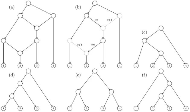
(29) 1.3. TREES AND NETWORKS IN PHYLOGENETICS of it, hence a duplication. Such duplication processes are important since they permit proteins to adquire new functions or to keep its original function when a mutation affects a gene. When the effect of the duplication for the population is either detrimental or it has a neutral (neither detrimental nor beneficial) effect, this sequence may get lost.. 1.3. Trees and networks in phylogenetics. A group of organisms are interrelated by ancestor and descendant relationships derived from “vertical” and “horizontal” processes as those we have seen in the previous section. A phylogenetic tree (see also Section 1.10) is a branching diagram illustrating the evolutionary history infered from a set of taxa reflecting vertical events like mutations. The use of phylogenetic trees limits the identification and visualization of more complex evolutionary scenarios. That is, the evolutionary processes like hibridizations, lateral gene transfer or recombinations can not be modelled by a tree structure. For this reason, phylogenetic networks were introduced in order to model the evolutionary history of a group of organisms where we can take into account both vertical and horizontal events. In the field of computational biology, the concepts of phylogenetic trees and networks appear in a multitude of ways depending on many factors [Semple and Steel (2003); Morrison (2011); Huson et al. (2010)]. Generically, they are graphs with certain restrictions that are used to model mathematically some biological problems related to the evolution of species. One of the main differences between different models lies on if one considers trees and networks which are rooted or unrooted. Commonly, rooted trees or networks are called evolutionary phylogenetic trees or networks to emphasize the existence of a common ancestor of all considered organisms and that the arcs can be interpreted as the evolution in time between the respective entities (see also Section 1.6). In this manuscript we will usually consider rooted phylogenetic trees and networks. Hence, the mathematical structure used to design a phylogenetic network is, generally, a rooted directed acyclic graph with labelled leaves (labelled rDAG, see Section 1.1). See an example of phylogenetic network depicted in Figure 1.4(a). It is usual to forbid elementary nodes, that is nodes with in-degree one (or zero) and out-degree one. In phylogenetic networks, nodes are classified depending on their in-degree; namely, nodes with in-degree one are called tree nodes nodes and nodes with in-degree at least two are called reticulation nodes. Then, a phylogenetic tree is a phylogenetic network without reticulation nodes (see Figure 1.4(c-f)). In this phylogenetic scenario, if there is a directed path u v between two nodes in a (phylogenetic) tree or network, we say that u is an ancestor of v, or also v is a descendant of u. Given two nodes u, v in a phylogenetic tree T , its lowest common ancestor (or LCA, for short), noted as LCAT (u, v), is their common ancestor that is descendant of every other common ancestor of them. This concept can be extended to consider the LCA of any set of nodes in a tree.. Displayed trees and switching The definitions of phylogenetic trees and networks as rDAGs are closely related. In fact, a phylogenetic tree is a particular case of a phylogenetic network. The main difference between them is that, in a phylogenetic tree, each pair of nodes are connected by exactly one (undirected) path, while in phylogenetic networks there can be many (undirected) paths connecting two given notes. The ultimate reason for the multiplicity of paths comes 11.

(30) CHAPTER 1. PRELIMINARIES from the fact that, in a phylogenetic network, a node (reticulation node) can have different parents. This tree-network relation becomes relevant to identify trees obtained from a network and, in the other way, networks obtained from a set of trees. A switching of a phylogenetic network is obtained by choosing, for each reticulation node in the network, an incoming arc to switch on and switch off all the others. Once this is done, we also recursively switch off all switched-on arcs whose target node has only switched-off outgoing arcs [Huson et al. (2010); Kelk and Scornavacca (2014)]. After applying all these switchings, if one removes the switched-off arcs one gets a tree. Notice also that some elementary nodes may appear and hence they must be contracted. If a tree can be obtained from this process from a network, we say that the tree is displayed by the network. See a complete example in Figure 1.4. (a). (b) on. of f. (c) on. of f. 1. 2. 3. 4. 1. (d). 1. 2. 3. 4. 1. (e). 2. 3. 4. 1. 2. 3. 4. 2. 3. 4. (f). 2. 3. 4. 1. Figure 1.4: (a) A phylogenetic network N defined in {1, 2, 3, 4}. (b) A switching of N . (c) A tree displayed by N derived from the chosen switching. Note that there are 2 switchedoff arcs and 4 nodes which become elementary and, consequently, they are suppressed. (d-f) The rest of trees displayed by N .. 1.4. Newick notation for trees and networks. The Newick format [Felsenstein (2004)] is a way to represent the topology (and the edge lengths if needed) of a phylogenetic tree using plain text. This is one of the most commonly used formats in software specific to bioinformatics. Later, in Cardona et al. (2008b) it was extended to encode phylogenetic networks.. Newick notation for phylogenetic trees We consider a rooted tree. To obtain the Newick string encoding the tree we proceed recursively in the following way. Each leaf is encoded by its label. Each internal node is encoded by a string starting with “(” followed by the list of encodings of each of its children 12.

(31) 1.4. NEWICK NOTATION FOR TREES AND NETWORKS (separated by commas) and then closing the parenthesis “)”; finally, if the internal node is labelled, this label is added as the last part of the string. The Newick string for the tree is the encoding associated to its root by the procedure above followed by the ending character ;. For example, the Newick strings that represent the 4 phylogenetic trees in Figure 1.4 are:. • ((1, (2, 3)), 4); for the tree in (c), • (((1, 2), 3), 4); for the tree in (d), • ((1, 2), (3, 4)); for the tree in (e), • (1, ((2, 3), 4)); for the tree in (f).. Newick notation for phylogenetic networks The Newick format can be generalized to consider phylogenetic networks. The extended Newick (or eNewick for short) [Cardona et al. (2008b)] is one of such generalizations. The principal idea of this version relies on transforming the network into a rooted tree (possibly multilabelled and with internal nodes labelled in some very specific way) such that the original network can be reconstructed from it. The Newick string of the obtained tree (with some special rules to encode labelled internal nodes) is the eNewick string of the original network. More precisely, to obtain the eNewick string which represents a phylogenetic network N we proceed as follows: let {H1 , . . . , Hm } be the set of hybrid nodes of N ordered in any fixed way. For each hybrid node H = Hi , let u1 , . . . , uk and v1 , . . . , vl be its set of parents and children, respectively. Then H is splitted in k different nodes where the first copy has u1 as its parent and v1 , . . . , vl as its children; and the other copies have (one for each) u2 , . . . , uk as their respective parent and have no children. Finally, each of the copies of H are labelled as [label]#[type]tag[: branch length] where:. • label (optional): string providing a labelling for the node. • type (optional): string indicating which is the corresponding event that the node models: hybridization indicated by H, or lateral gene transfer indicated by LGT. • tag (mandatory): integer i identifying the node H = Hi . • branch length (optional): number indicating the length of the arc from the considered copy of H to its parent.. For example, the eNewick of the phylogenetic network depicted in Figure 1.4 (a) is (((1, (2)#H2), ((#H2, 3))#H1), (#H1, 4)); where H1 and H2 represents the above and the up and down reticulation nodes in the network, respectively. 13.

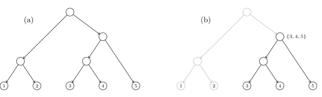
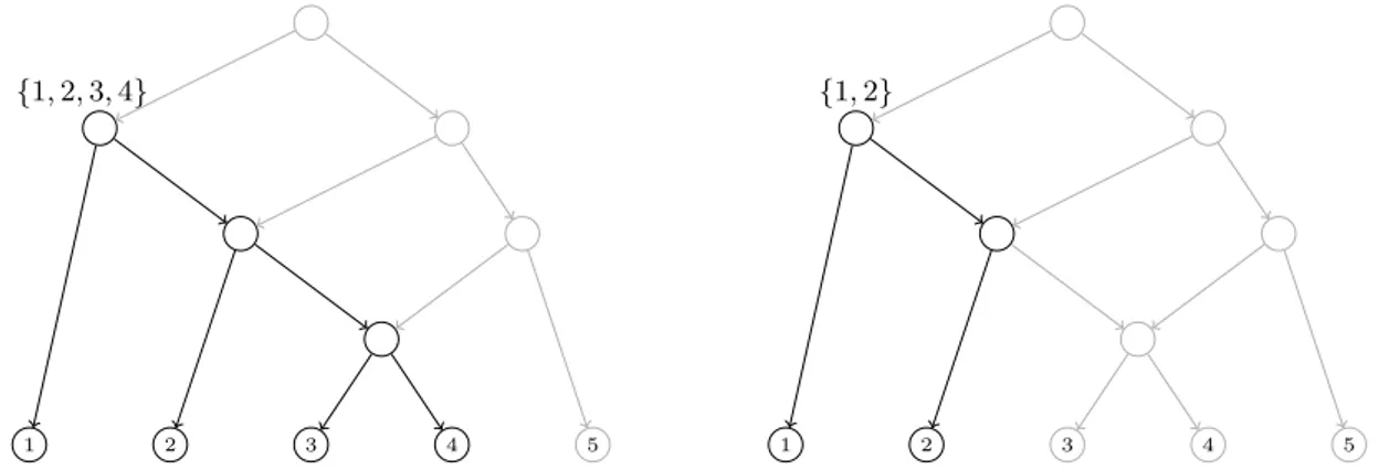
(32) CHAPTER 1. PRELIMINARIES. 1.5. Decomposition of trees and networks. In this section we describe how a “global object”, describing all the evolutionary relations among a set of species, can be decomposed into “local objects” describing relations among restricted subsets of species. Namely, we will focus on clusters and triples. Such objects only make sense in the setting of rooted trees but they have their unrooted counterparts, splits and quartets. We will also show how these concepts can be extended to networks, where one needs to consider different kinds of clusters and generalize triples to what we call trinets. In the classical case of phylogenetic trees, clusters and triples are enough to encode trees; that is, one can recover the tree from this data. However, for phylogenetic networks, it is no longer true and one needs to impose restrictions on the networks in order to recover them from this “local data” [Cardona et al. (2008c, 2009b,c,e)].. Clusters Given T = (V, E) a phylogenetic tree labelled on a finite set S, and a node u ∈ V , the cluster of u, denoted by CT (u), is the set of labels of all the descendant leaves of u. The set of clusters defined by T , denoted by C(T ), is the set of clusters of all its nodes: C(T ) = {CT (u) : u ∈ V } (see Figure 1.5). Notice that the clusters of nodes in T satisfies that: • The cluster of a leaf is the singleton composed of its label. • The cluster of the root is the set of labels of all leaves in the tree. • The cluster of a node is the disjoint union of the clusters of its children.. (a). (b) {3, 4, 5}. 1. 2. 3. 4. 5. 1. 2. 3. 4. 5. Figure 1.5: (a) A phylogenetic tree T such that C(T ) = {{1}, {2}, {3}, {4}, {5}, {1, 2}, {3, 4}, {3, 4, 5}, {1, 2, 3, 4, 5}}. (b) Depiction of the cluster defined by a specific node in T . We can also talk of clusters in phylogenetic networks. Notice that in this case there can be more than one path from an internal node to a leaf. This fact produces different kinds of clusters that can be considered. We say that a phylogenetic network N defines or displays a cluster C in hardwired sense if C is the set of descendants leaves of a node in N (which is the usual concept of cluster used in trees). On the other hand, we say that N defines or displays C in softwired sense if C is the cluster of a node in some tree displayed by N (see Section 1.3). Note that if N displays C in hardwired sense, then it is displayed also in softwired sense. Indeed, let u be a node with hardwired cluster C. A tree displayed by N and where the cluster of u is C can be constructed by considering the following 14.

(33) 1.5. DECOMPOSITION OF TREES AND NETWORKS switching. For each reticulation node h, if h is not a descendant of u, keep switched on any incoming arc; if h is a descendant of u, keep switched on any incoming arc (v, h) such that v is also a descendant of u. It follows easily that for each descendant leaf of u there exists a path formed by switched on arcs. Notice, however, that softwired clusters need not be hardwired clusters; see Figure 1.6.. {1, 2, 3, 4}. 1. {1, 2}. 2. 3. 4. 5. 1. 2. 3. 4. 5. Figure 1.6: A phylogenetic network displays in hardwired sense the cluster {1, 2, 3, 4} (left) and in softwired sense the cluster {1, 2} (right). Note that, the cluster {1, 2} is only displayed by N in softwired sense.. Triples A triple on three different labels x, y, z ∈ S is a rooted phylogenetic tree on {x, y, z}. Figure 1.7 depicts the only four possible (non-isomorphic) triples defined on x, y, z, together with their Newick notation (see Section 1.4). If we consider only binary trees, the triple (x, y, z) doesn’t have to be taken into consideration. The other ones, ((x, y), z), ((y, z), x) and ((x, z), y) are commonly represented as xy|z, yz|x and xz|y, respectively.. x. y. ((x, y), z). z. y. z. x. x. ((y, z), x). z. y. x. ((x, z), y). y. z. (x, y, z). Figure 1.7: All possible triples defined on x, y, z. We say that a phylogenetic tree T on S defines or displays a triple on x, y, z ∈ S if there exists a subgraph of T homeomorphic to the given triple. The triple on x, y, z ∈ S displayed by T is denoted by Tx,y,z . The set of triples displayed by T is denoted by Γ(T ); see Figure 1.8. That is Γ(T ) = {Tx,y,z : {x, y, z} ⊂ S}. Analogously as what we did in the case of clusters, we can also define the set of triples defined or displayed by a phylogenetic network. In this case, we need to generalize the concept of triple used on trees and consider trinets. This last concept will be analyzed later in Chapter 4. A set of triples T defined on a set of taxa S is called dense if for each subset of three taxa in S there is at least one triple in T defined on these three taxa. This notion of dense set 15.

(34) CHAPTER 1. PRELIMINARIES. (a). 1. (b). 2. 3. 4. 5. 1. 2. 3. 4. 5. Figure 1.8: (a) Phylogenetic tree, we call T , such that its set of displayed triples are Γ(T ) = {((1, 2), 3), ((1, 2), 4), ((1, 2), 5), (1, (3, 4)), (1, (3, 5)), (1, (4, 5)), (2, (3, 4)), (2, (3, 5)), (2, (4, 5)), ((3, 4), 5)}. (b) Depiction of how the triple (1, (4, 5)) is displayed by T . of triples will become significant in the reconstruction problem of phylogenetic networks (see Section 1.9). Recall that two phylogenetic trees defined on S are isomorphic if, and only if, they have the same set of clusters, and also if, and only if, they define the same set of triples [Theorems 3.5.2 and 6.4.1 in Semple and Steel (2003)]. Then, the set of clusters and triples defines with unicity or encodes a phylogenetic tree. Actually, the descriptions of a phylogenetic tree T on S by means of C(T ) and Γ(T ) are equivalent, through the following result [Lemma 9.1 in Dress et al. (2012)]. Theorem 1.1. Let T be a phylogenetic tree T on S. For every non-empty subset C ⊂ S, C ∈ C(T ) if, and only if, ((c, c0 ), x) ∈ Γ(T ), for every c, c0 ∈ C and x ∈ S \ C.. 1.6. Classification of phylogenetic networks. There are a multitude of definitions for many kinds of phylogenetic networks. We can even find different names to design the same kind of phylogenetic network and, what is worse, different kinds of networks with the same name. The classification of phylogenetic networks may depend on a large amount of factors, as we shall shortly see. Then, it is (at the moment) quite impossible to find a general classification that can be used by all the scientific community. Based on Morrison (2011), Huson et al. (2010), Huson and Scornavacca (2011), we can find two kinds of classifications. The first one divides the whole set of phylogenetic networks into two big blocks: • Rooted vs. unrooted networks. This classification is based on the underlying graph model that is used (directed vs. undirected) and, biologically, it corresponds to assuming or not that the least common ancestor of a set of species is known. • Abstract or data-display networks vs. explicit or evolutionary networks. The abstract or data-display networks are those whose edges or arcs cannot be interpreted biologically and they are just used as a visualization tool of possible incompatibilities. On the other hand, the explicit or evolutionary networks describe an evolutionary scenario where the nodes and edges should represent species and evolutionary events between them. Other possible classifications depend on the biological phenomenon under study (for instance, recombination or hybridization networks), the data used to build the networks 16.

(35) 1.7. TOPOLOGICAL RESTRICTIONS (like split, cluster or consensus networks) or the topological constraints they must satisfy (such as galled trees, tree-child, tree-sibling or level-k networks). Next section is devoted to the study of this last group of restrictions.. 1.7. Topological restrictions. The problem of reconstructing phylogenetic networks from biological data (or certain substructures like clusters or trees) commonly leads to NP-problems, and even NP-hard ones, when no restriction on the space of phylogenetic networks is imposed. In order to make the reconstruction process feasible, it is usual to introduce topological restrictions on the space of phylogenetic networks. The close link between the mathematical structure, to be used in solving the problem, and the biological interpretation, that lies behind, appears here with more strength. That is, the main goal is to obtain a mathematical model that, on the one hand, can be analyzed mathematically and, on the other hand, it models accurately the real biological situation. In the rest of this section, following Morrison (2013), we discuss some of the restrictions that usually appear in the literature related to phylogenetic trees.. Restrictions on degrees Restrictions on the degrees of the nodes can be imposed either on their indegree, their outdegree, or both. A typical condition related to degrees is forbidding the existence of elementary nodes, since they cannot be recovered. Another condition is not allowing nodes to have indegree or outdegree greater than two. The biological motivation behind this assumption is that nodes with indegree or outdegree greater than two are only due to the lack of information, and having more knowledge would resolve that polytomy. We say that a phylogenetic network is binary if its tree nodes have indegree one and outdegree two and its reticulation nodes have indegree two and outdegree one. When this condition is only fulfilled for reticulation nodes, we say that it is semibinary.. Time-consistent networks Roughly speaking, a phylogenetic network is time-consistent if it can be drawn in such a way that arcs leading to a reticulation node are horizontal and arcs leading to tree nodes point downwards (see Figure 1.9(a)). That is, one can assign times to the nodes of the network in a way that strictly increases on arcs whose endpoint is a tree node (which should model speciation events, that take time to happen) and is constant on arcs whose endpoint is a reticulation node (which models interactions between coexistent species). Temporal consistency becomes a key factor in the reconciliation problem between gene trees and species trees, as we shall see in Chapter 5. Formally, a phylogenetic network N = (V, E) is time-consistent [Baroni et al. (2006)] if it admits a temporal assignment: a mapping τ : V → N such that: 17.

(36) CHAPTER 1. PRELIMINARIES • τ (r) = 0, where r is the root of N . • τ (u) = τ (v) if (u, v) ∈ E and v is a reticulation node. • τ (u) < τ (v) if (u, v) ∈ E and v is a tree node. Figure 1.9 depicts two phylogenetic networks. The network in (a) is time-consistent and the number close to each node indicates its assignment in a valid mapping. In contrast, the network in (b) is not time-consistent: it is impossible to define a temporal assignment because the two parents of the hybrid node are tree nodes connected by an arc. (b) (a) 1 2. 0 1. 1. 2. 1 2. 2. 3. 1. 2. 3. Figure 1.9: A time-consistent phylogenetic network (a) and a non time-consistent phylogenetic network (b). While the definition above of time-consistency is the most used and well-known, Górecki (2004) uses a slightly different one. First, he considers what he calls species graphs, given by a tree together with a set of extra arcs that are added modelling lateral gene transfer. In this setting, the condition on the time assignment is only taken into account for nodes that are adjacent to these extra arcs. A similar definition will be used in Chapters 4 and 5 in our own model of networks.. Tree-child and tree-sibling networks A phylogenetic network is tree-child when every non-extant species has some descendant through mutation [Cardona et al. (2009e)]. Mathematically, this means that each internal node has a child that is a tree node. Both phylogenetic networks depicted in Figure 1.9 are tree-child and the one depicted in Figure 1.10 is not tree-child because it has one node whose two children are hybrid nodes. Some problems, as the Tree Containment problem (deciding if a given phylogenetic tree is embedded in a given phylogenetic network), the reconstruction problem from trinets or the reconstruction from path-lengths distances between taxa [Bordewich and Semple (2015a)], among others, can be solved in polynomial time if the space of solutions is restricted to tree-child networks, while they are NP-hard for generic phylogenetic networks [Cardona et al. (2009e, 2010c)].. 1. 2. 3. Figure 1.10: A non tree-child phylogenetic network. 18.

(37) 1.7. TOPOLOGICAL RESTRICTIONS A phylogenetic network is tree-sibling if at least one of the species involved in a reticulation event has some descendant through mutation [Nakhleh (2004); Cardona et al. (2008a)]. This is, each hybrid node has at least one sibling (a child of one of its parents) that is a tree node. Note that every tree-child network is, in particular, a tree-sibling network. Figure 1.11 shows a tree-sibling network that is, non tree-child (a), and a non tree-sibling network (b); notice that the parent of the leaf 3 is an hybrid node whose two sibling nodes are also hybrid. (a). 1. (b). 2. 3. 4. 1. 2. 3. 4. 5. Figure 1.11: (a) A tree-sibling phylogenetic network, (b) a non tree-sibling phylogenetic network.. Stable networks A node u in a phylogenetic network is visible if there exists at least one leaf l such that all paths from the root to l pass through u. In this case, the node u is said to be a stable ancestor of l. Then, a phylogenetic network is reticulation-visible [Van Iersel et al. (2010b)] or stable [Gambette et al. (2015a); Huber et al. (2015a)] if each reticulation node is visible. Using the definition of visible nodes, a tree-child network can be redefined as a network where every node (not only reticulation nodes) is visible. Figure 1.12 shows a reticulation-visible network (a), where each hybrid node is a stable ancestor of a leaf (node a is a stable ancestor of 1, node b is a stable ancestor of 2 and node c is a stable ancestor of 3), and a non reticulation-visible network (b) where one hybrid node, node b, is not visible. (a). (b). b b. c. a. 1. 2. 3. a. c. 1. 2. 3. Figure 1.12: (a) A reticulation-visible network, (b) a non reticulation-visible network. Thanks to the reticulation-visible networks, it is proved in Bordewich and Semple (2015b) that Tree Containment problem becomes tractable. Some other kinds of networks based on the concept of stability are nearly-stable networks [Gambette et al. (2015a)], genetically19.

(38) CHAPTER 1. PRELIMINARIES stable networks [Gambette et al. (2015b)] and stable-child networks [Gunawan and Zhang (2015)].. Galled trees and networks A phylogenetic network is said to be a galled tree if each biconnected component has at most one reticulation node [Gusfield et al. (2003)]. It can also defined as one network such that each node belongs to at most one reticulation cycle –pair of paths with same origin and destination nodes and with disjoint intermediate nodes. From a biological point of view, this can be translated as saying that the reticulation events are independent. Galled trees have been extensively used in the reconstruction problem [Jansson and Sung (2006); Huber et al. (2011); Gambette et al. (2015c)]. Galled trees can be generalized in several ways. One of these generalizations, level-k networks, will be analyzed in the next section. Another such generalization is to consider galled networks [Huson and Klöpper (2007)], where the following restriction is introduced. For each reticulation node u and each pair of nodes ui , uj such that both (ui , u) and (uj , u) are arcs of the network, there is a non directed cycle containing ui , uj and such that the other nodes of the cycle are tree nodes, see Figure 1.13. This corresponds to a biological scenario in which reticulate events are quite rare [Huson et al. (2009)]. Among others, galled networks permit to solve the Cluster Containment problem (deciding if a given subset of leaves is a cluster of some phylogenetic tree embedded in the network) in polynomial time [Huson et al. (2009)], while it is an NP-problem for generic rooted networks [Kanj et al. (2008)].. 1. 2. 3. 4. 5. Figure 1.13: A galled network which is not a galled tree.. Level-k networks The level of a network is, roughly speaking, a bound on the number of reticulations that can be mutually dependent [van Iersel and Kelk (2011)]. This is a measure to quantify the complexity of the network by means of biconnected components. More formally, a (binary) phylogenetic network is a level-k network if each biconnected component has at most k reticulation nodes [Choy et al. (2005); Jansson and Sung (2006)]. See Figure 1.14. Notice that galled trees are nothing but level-1 networks, and the biological meaning of level-k networks can also be understood as a generalization of those in the sense that the level describes up to which extent the reticulations are dependent. See Gambette et al. (2009), Gambette et al. (2012), Habib and To (2012), Van Iersel et al. (2009a), Van Iersel 20.

(39) 1.7. TOPOLOGICAL RESTRICTIONS et al. (2009b) for some reconstruction problems which have can be efficiently solved using the level constraint.. 1. 2. 3. 4. 5. Figure 1.14: A level-2 phylogenetic network.. Tree-based networks The notion of tree-based networks is important to differentiate networks which should properly be viewed as networks from those that should be viewed as “augmented” trees, i.e. trees with some extra arcs being added between their arcs. This distinction is important from the biological point of view in order to determine which is the evolutionary process under study, especially in some groups of organisms such as the prokaryotes [Dagan and Martin (2006); Doolittle and Bapteste (2007); Martin (2011)]. Although there are similar definitions for these networks, here we will use the one given in Francis and Steel (2015b), where a phylogenetic network is said to be tree-based if it can be obtained from a tree with same set of leaves by inserting extra arcs between the arcs of the tree. Here, to insert an extra arc between two given arcs, one splits each of these arcs into an elementary path of length two and then connects the introduced elementary nodes with an arc. See also Szöllősi et al. (2013). For example, all phylogenetic networks depicted in this section are tree-based networks. On the other hand, an example of a non-tree based network is presented in Figure 2(iii) of Francis and Steel (2015b) and reproduced in Figure 1.15.. 1. 2. 3. Figure 1.15: A non-tree based phylogenetic network.. 21.

(40) CHAPTER 1. PRELIMINARIES. Regular and normal networks A phylogenetic network is regular if no two distinct nodes have the same cluster, and the cluster of a node u is contained in the cluster of another one v if, and only if, there is a path from the former to the latter v to u [Baroni et al. (2005); Baroni and Steel (2006)]. In other words, a network is regular if it isomorphic to the Hasse diagram of its set of clusters. A phylogenetic network is said to be normal if it is simultaneously tree-child and regular [Willson (2010)].. 1.8. Metrics on phylogenetic networks. Metrics to measure the difference between networks play a key role in different tasks such as the detection of incongruences between gene trees and species trees, and the comparison of networks reconstructed from different sets of data or using different algorithms. Hence, these metrics are of great use in determining the degree of success of the reconstruction algorithms and of the recovery of the characteristics of the networks. Based on the idea of comparing a reconstructed network with the true evolutionary history, some publications refer to such distances or metrics as error-distances or error-metrics, see [Moret et al. (2002); Linder et al. (2003)]. Contrarily to phylogenetic trees, networks can present multiple evolutionary paths from internal nodes to leaves, making their comparison much more complex. Since there can be non isomorphic networks whose distance is zero, the distances designed to work on phylogenetic trees do not in general work on phylogenetic networks. Hence, one must either restrict the space of phylogenetic networks to consider or define new metrics. Let us consider a class C of phylogenetic networks. A metric on C is a mapping d : C × C → R such that, for all A, B, C ∈ C: (a) Non-negativity: d(A, B) ≥ 0, (b) Separation: d(A, B) = 0 if and only if, A ∼ = B, (c) Symmetry: d(A, B) = d(B, A), (d) Triangular inequality: d(A, C) ≤ d(A, B) + d(B, C).. The search of a sound metric on the set of all phylogenetic networks that can be computed efficiently seems to be an impossible task. In fact, the isomorphism problem for tree-sibling time-consistent networks (which is a quite restrictive case) is polynomially equivalent to the graph isomorphism problem, hence it is thought to be neither P nor NP-complete [Cardona et al. (2009a)]. Several metrics have been introduced so far in the literature. See [Warnow et al. (2003), Moret et al. (2004), Baroni et al. (2005), Cardona et al. (2008c), Cardona et al. (2008a), Cardona et al. (2009b), Cardona et al. (2009e), Cardona et al. (2009c)]. Next, we review some of them in more detail. 22.