Feature transformations for improving the performance of selection hyper heuristics on job shop scheduling problems

Texto completo

(1)Instituto Tecnológico y de Estudios Superiores de Monterrey Monterrey Campus. School of Engineering and Sciences. Feature Transformations for Improving the Performance of Selection Hyper-heuristics on Job Shop Scheduling Problems A dissertation presented by. Fernando Garza Santisteban Submitted to the School of Engineering and Sciences in partial fulfillment of the requirements for the degree of Master of Science in Computer Science. Monterrey, Nuevo León, May, 2019.

(2) Declaration of Authorship. I, Fernando Garza Santisteban, declare that this dissertation entitled Feature Transformations for Improving the Performance of Selection Hyper-heuristics on Job Shop Scheduling Problems, and the work presented in it are my own. I also confirm that: • This work was done wholly or mainly while in candidature for a research degree at this University. • Where any part of this dissertation has previously been submitted for a degree or any other qualification at this University or any other institution, this has been clearly stated. • Where I have consulted the published work of others, this is always clearly attributed. • Where I have quoted from the work of others, the source is always given. With the exception of such quotations, this dissertation is entirely my own work. • I have acknowledged all main sources of help. • Where the dissertation is based on work done by myself jointly with others, I have made clear exactly what was done by others and what I have contributed myself.. Fernando Garza Santisteban Monterrey, Nuevo León, May, 2019. ©2019 by Fernando Garza Santisteban All Rights Reserved ii.

(3) Dedication. To God, my family, and friends. Thanks for all your support, patience and reassurance throughout the development of this research.. iii.

(4) Acknowledgements. This research would not have been possible without the help of my advisors. I would like to praise the instructional and supportive efforts of professors Terashima, Amaya and Ortiz. I am very thankful for your time and dedication. A special mention is due to professor Taillard, which has kindly provided the source code of an instance generator used for this research. Also, thankfulness is due to both Tecnológico de Monterrey for their support on tuition and CONACyT for the economic scholarship provided throughout my studies.. iv.

(5) Feature Transformations for Improving the Performance of Selection Hyper-heuristics on Job Shop Scheduling Problems by Fernando Garza Santisteban Abstract Solving Job Shop (JS) scheduling problems is a hard combinatorial optimization problem. Nevertheless, it is one of the most present problems in real-world scheduling environments. Throughout the recent computer science history, a plethora of methods to solve this problem have been proposed. Despite this fact, the JS problem remains a challenge. The domain itself is of interest for the industry and also many operations research problems are based on this problem. The solution to JS problems is overall beneficial to the industry by generating more efficient processes. Authors have proposed solutions to this problem using dispatching rules, direct mathematical methods, meta-heuristics, among others. In this research, the application of feature transformations for the generation of improved selection constructive hyper-heuristics (HHs) is shown. There is evidence that applying feature transformations on other domains has produced promising results; Also, no previous work was found where this approach has been used for the JS domain. This thesis is presented to earn the Master’s degree in Computer Science of Tecnológico de Monterrey. The research’s main goals are: (1) the assessment of the extent to which HHs can perform better on JS problems than single heuristics, and that they are not specific to the instances used to train them; and (2), the degree to which HHs generated with feature transformations are revamped. Experiments were carried out using instances of various sizes published in the literature. The research involved profiling the set of heuristics chosen, analyzing the interactions between the heuristics and feature values throughout the construction of a solution, and studying the performance of HHs without transformations and by using two transformations found in the literature. Results indicate that for the instances used, HHs were able to outperform the results achieved by single heuristics. Regarding feature transformations, it was found that they induce a scaling effect to feature values throughout the solution process, which produces more stable HHs, with a median performance comparable to HHs without feature transformations, but not necessarily better. Results are conclusive in terms of the objectives of this research. Nevertheless, there are several ideas that could be explored to improve the HHs, which are outlined and discussed in the final Chapter of the thesis. The following major contributions are derived from this research: (1) applying a selection constructive HH approach, with feature transformations, to the JS domain; (2) the rationale behind the JS subproblem dependance in terms of the solution paths followed by the heuristics, which has a great impact in the training process of the HHs; (3) a method to determine the most suitable parameters to apply feature transformations, which could be extended for other domains of combinatorial optimization problems; and (4) a framework for studying HHs in the Job Shop domain. v.

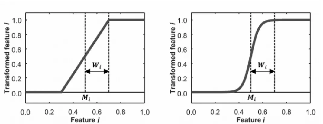
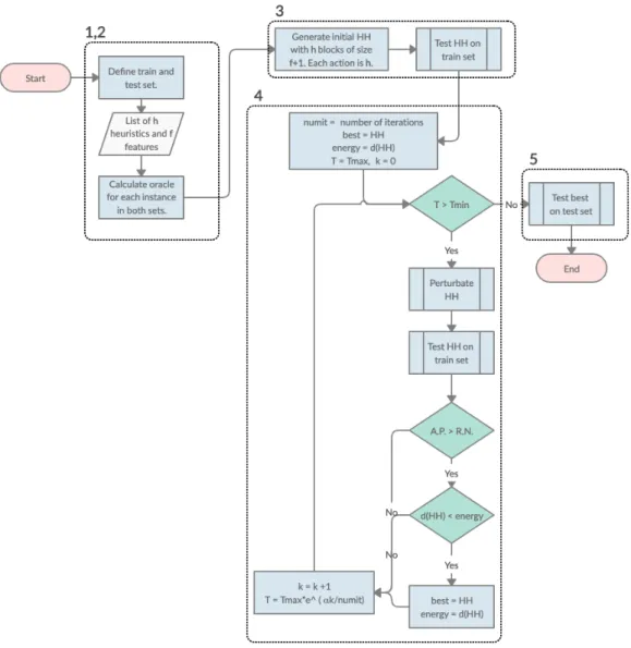
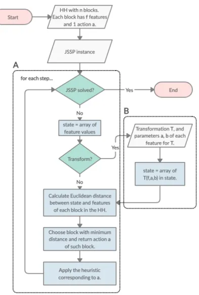
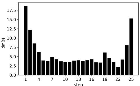
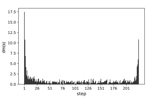
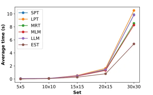
(6) List of Figures 3.1 3.2 3.3 3.4. 3.5. 5.1 5.2 5.3 5.4 5.5. 6.1 6.2. Example of a HH with 4 blocks. Features fiq correspond to specific actions ri , the latter representing a call to a specific heuristic, in this case, rules 1-4. . Possible operations done by the SA over a candidate solution (a): remove block (b), add block (c), randomize the feature of a block (d). . . . . . . . . . Linear (left) and S-shaped (right) transformations. Mi and Wi represent the mid-point and half-width, respectively. Figure taken from the research published by Amaya et al. [4]. . . . . . . . . . . . . . . . . . . . . . . . . . . . Block diagram showing the process to train a single HH. Each area has a number that corresponds to a step described in Section 3.7. Also, the diagram showing how to test a HH is shown in Figure 3.5. Note that A.P. stands for acceptance probability and R.N. for a random number. Also, the method by which a HH is perturbated is described in Section 3.4. . . . . . . . . . . . . . Block diagram showing the process to apply a HH to a JSSP instance. Note that area A is the general process without transformations, and area B is for the case when a transformation is applied. Hence, a HH that involves transformations goes through A and B, while one without transformations only goes through A. . . . . . . . . . . . . . . . . . . . . . . . . . . . . . . . . . . . . Average of dm(s) (given in Equation 5.1) at each step of the construction of a schedule for instances of size 5 ⇥ 5. . . . . . . . . . . . . . . . . . . . . . Average of dm(s) (given in Equation 5.1) at each step of the construction of a schedule for instances of size 15 ⇥ 15. . . . . . . . . . . . . . . . . . . . . Average time (in seconds) that each heuristic takes to construct a solution for sets of 100 instances of different sizes. . . . . . . . . . . . . . . . . . . . . . Performance of hyper-heuristics (30 runs) trained with 30 instances of size 5 ⇥ 5 (TRAIN), and tested on a set of 5 (T5), 10 (T10) and 20 (T20) instances of same size. . . . . . . . . . . . . . . . . . . . . . . . . . . . . . . . . . . . Performance of hyper-heuristics (30 runs) trained with 30 instances of size 15 ⇥ 15 (TRAIN), and tested on a set of 5 (T5), 10 (T10) and 20 (T20) instances of same size. . . . . . . . . . . . . . . . . . . . . . . . . . . . . . . Average of uhi /phi for all h 2 H of a 15 ⇥ 15 instance. . . . . . . . . . . . . . Feature values for an instance (size 15 ⇥ 15): (a) APT, (b) DPT, (c) NAPT, (d) NJT, (e) DNPT, and (f) SLACK. In each subplot, every heuristic is plotted with a different marker. The horizontal axis corresponds to each step of the solution process. . . . . . . . . . . . . . . . . . . . . . . . . . . . . . . . . vi. 21 25 28. 31. 32 40 41 43 44 45 47. 48.

(7) 6.3 6.4 6.5. 6.6. 7.1 7.3. 7.2. 7.4 7.5 7.6 7.7. 7.8. Performance of hyper-heuristics (30 runs) over a test set with 5 instances of size 15⇥15. Hyper-heuristics were trained on 30 instances of size 5⇥5 (Left) and of size 15 ⇥ 15 (Right) with 100 iterations. d(HH) is given in Equation 3.2. Feature values (DNPT and NJT) for sets with 30 instances of different sizes. Red ’x’ markers: 5 ⇥ 5 instances; Blue ’.’ markers: 15 ⇥ 15 instances; Green ’+’ markers: 30 ⇥ 30 instances. . . . . . . . . . . . . . . . . . . . . . . . . Performance of hyper-heuristics (30 runs) with a different number of iterations: 10, 100, 1000. Data is shown for training (TR) and testing (TE). In all cases, 30 instances of size 15 ⇥ 15 were used for training. d(HH) is given in Equation 3.2. . . . . . . . . . . . . . . . . . . . . . . . . . . . . . . . . . . Performance of hyper-heuristics (30 runs) with a different number of iterations: 10, 100, 1000. Data is shown for training (TR) and testing (TE). Each hyper-heuristic was trained with 30 instances of sizes 5 ⇥ 5 and 15 ⇥ 15. d(HH) is given in Equation 3.2. Statistical tests are reported in Appendix A, Table A.1. . . . . . . . . . . . . . . . . . . . . . . . . . . . . . . . . . . . . Original (marker ‘.’) and ST transformed (markers ‘x’) values of DNPT and NJT features for 30 instances of size 15 ⇥ 15. . . . . . . . . . . . . . . . . . Original (gray) and LT transformed (black) feature values for all heuristics when solving an instance of size 15 ⇥ 15. Horizontal axis of each sub-plot is the step. Features: (a) APT, (b) NJT, (c) DPT, (d) SLACK, (e) DNPT, and (d) NAPT. . . . . . . . . . . . . . . . . . . . . . . . . . . . . . . . . . . . . . Original (gray) and ST transformed (black) feature values for all heuristics when solving an instance of size 15 ⇥ 15. Horizontal axis of each sub-plot is the step. Features: (a) APT, (b) NJT, (c) DPT, (d) SLACK, (e) DNPT, and (d) NAPT. . . . . . . . . . . . . . . . . . . . . . . . . . . . . . . . . . . . . . . Original (gray) and LT transformed (black) values for all heuristics at step i of the solution of an instance of size 15 ⇥ 15. The range of the LT is [0,0.1]. Feature: APT. . . . . . . . . . . . . . . . . . . . . . . . . . . . . . . . . . . Traning results (30 runs) of experiments described in Table 7.1. d(HH) given in Equation 3.2. . . . . . . . . . . . . . . . . . . . . . . . . . . . . . . . . . Test results (30 runs) of experiments described in Table 7.1. d(HH) given in Equation 3.2. . . . . . . . . . . . . . . . . . . . . . . . . . . . . . . . . . . Results (30 runs) of experiments for validating the proposed approach to tune transformations. Training set: 30 instances (5 ⇥ 5). Testing set: 5 instances (15⇥15). 1000 iterations were carried out in each of the training experiments, accordingly. Statistical tests are reported in Appendix A, Table A.2. . . . . . Testing performance of hyper-heuristics trained for 100 and 1000 iterations, on 30 instances of size 5 ⇥ 5, with and without transformations. Test set: 10 (different) instances of size 5 ⇥ 5. O: Hyper-heuristics without transformations. L: Hyper-heuristics with linear transformation, following the method described in Section 7.4. The number corresponds to the number of iterations done during training. . . . . . . . . . . . . . . . . . . . . . . . . . . . . . .. vii. 50 51. 52. 53 57. 58. 58 59 61 61. 63. 64.

(8) 7.9. Results for HHs trained with 1000 iterations, on 30 instances of size 15 ⇥ 15, with and without transformations, when tested on a set of 5 benchmarking instances of the same size, proposed by Taillard. O are HHs without transformations, L with the linear transformation, S with the S transformation. TR stands for training and TE for testing. Parameters of the transformations are reported in Table 7.3. Statistical tests are reported in Appendix A, Table A.3, and results for each replica in Appendix C. . . . . . . . . . . . . . . . . . . . 7.10 Results for 30 HHs trained with 1000 iterations, on 10 instances of size 15 ⇥ 15, with and without transformations, when tested on a set of 10 benchmarking instances of size 15 ⇥ 15, proposed by Lawrence et al. [72]. O: HHs without transformations; L: HHs linear transformation; S: HHs with S-shaped transformation. Parameters of the transformations are reported in Table 7.3. . 7.11 Results for HHs trained with 1000 iterations, on 10 instances of size 15 ⇥ 15, with and without transformations, when tested on a set of 10 benchmarking instances of size 20 ⇥ 15, proposed by Demirkol et al. [35]. O: HHs without transformations; L: HHs linear transformation; S: HHs with S-shaped transformation. Parameters of the transformations are reported in Table 7.3. . . . . B.1 Illustration of how energy diminishes throughout the number of iterations when applying the training algorithm. Each line represents a different HH trained with 30 instances of size 15 ⇥ 15. In total, 30 replicas are shown. . . .. viii. 65. 69. 69. 78.

(9) List of Tables 2.1 2.2. Example of the increasing complexity of JSS problem with n jobs and m = 1. Comparison of average times for finding optimal solutions to 3⇥3 and 15⇥15 instances in single and 8-threaded MIP optimizers, as reported by Ku et al. [67]. Each set contains 10 instances, reported time corresponds to average time for one instance. n.o.s stands for the number of optimal solutions achieved in the set. . . . . . . . . . . . . . . . . . . . . . . . . . . . . . . .. 3.1. Example of a JSSP instance of size 3 ⇥ 3. . . . . . . . . . . . . . . . . . . .. 4.1. Experiments to test time complexity of the SA training process with different sizes of instances and the number of instances to be used for each set. . . . . Experiments for stage two with defined sizes for training, and with a test set of 5 instances of size 15 ⇥ 15. . . . . . . . . . . . . . . . . . . . . . . . . .. 4.2 5.1 5.2. 5.3 5.4. 6.1 7.1. Performance results for every h 2 H for 100 instances of different sizes. . . . Comparison of the random hyper-heuristic (RHH) against the best makespan for instances of sizes 5 ⇥ 5 and 15 ⇥ 15. w: number of times RHH won, dw : mean difference of instances where RHH won, t: number of times RHH was tied, l: number of times RHH lost, dl : mean difference of instances where RHH lost, maxd : maximum difference throughout the set, mind : minimum difference throughout the set. . . . . . . . . . . . . . . . . . . . . . . . . . . Number of times that each heuristic was selected during the solution process. Data given corresponds to instances where the random hyper-heuristic (RHH) outperformed the best standalone heuristic. . . . . . . . . . . . . . . . . . . Average time (in seconds) required for training with SA throughout 5 iterations, for a different number of instances of different sizes. The marked cell corresponds to the configuration of training experiments that will be taken into account as an upper limit throughout the thesis. . . . . . . . . . . . . . . Time required to train a hyper-heuristic with 30 instances of sizes 5 ⇥ 5 and 15 ⇥ 15, with a different number of iterations. . . . . . . . . . . . . . . . . . Experiments for analyzing the effect of combining transformations. O: no transformation. S: S-Shaped. L: Linear. In all cases, the remaining features were used in their original domain (i.e. without transformations). . . . . . . .. ix. 11. 12 26 35 35 39. 42 42. 42 53. 60.

(10) 7.2. 7.3. Sample results yielded by the tuning approach when applied to the L transformation, on 30 instances of size 5 ⇥ 5, for the set of heuristics studied in this research. a: Lower bound of the transformation range. b: Upper bound of the transformation range. . . . . . . . . . . . . . . . . . . . . . . . . . . . . . . Tuning method for L, S and L/S transformations, on 30 instances of size 15 ⇥ 15. S: S-Shaped transformation, L: linear transformation, [a,b]: range of influence of a transformation. . . . . . . . . . . . . . . . . . . . . . . . . . .. 62 65. A.1 Wilcoxon’s signed rank sum test over the results from experiments of S2 (Figure 6.6), at ↵ = 0.05. The result is either Same or Different meaning the test implies that the experiments come from the same or from different distribution. 76 A.2 Wilcoxon’s signed rank sum test over the results from experiments of S4 (Figure 7.7), at ↵ = 0.05. The result is either Same or Different meaning the test implies that the experiments come from the same or from different distribution. 76 A.3 Wilcoxon’s signed rank sum test over the results from experiments of S4 (Figure 7.9), at ↵ = 0.05. The result is either Same or Different meaning the test implies that the experiments come from the same or from different distribution. 77 C.1 Results of confirmatory experiments of S4 (Figure 7.3) for 30 replicas. Trained without transformations (Original), with Linear (LT) and S-Shaped (ST) transformations, with 30 instances of size 15⇥15 and tested over the 5 benchmarking instances of size 15 ⇥ 15. . . . . . . . . . . . . . . . . . . . . . . . . . .. x. 79.

(11) Contents Abstract. v. List of Figures. viii. List of Tables. x. 1. Introduction 1.1 Motivations . . . . . . . . . . . . . . . . . . . 1.2 The JSS problem . . . . . . . . . . . . . . . . 1.2.1 Survey of Related Solution Approaches 1.2.2 Hyper-heuristic Formulation . . . . . . 1.2.3 Feature Transformations . . . . . . . . 1.3 Hypothesis . . . . . . . . . . . . . . . . . . . 1.4 Objectives . . . . . . . . . . . . . . . . . . . . 1.5 Contributions . . . . . . . . . . . . . . . . . . 1.6 Organization of the Document . . . . . . . . .. . . . . . . . . .. 1 1 2 3 4 4 5 5 6 7. 2. Theoretical Framework 2.1 Scheduling . . . . . . . . . . . . . . . . . . . . . . 2.1.1 Deterministic Models . . . . . . . . . . . . . 2.1.2 Stochastic Models . . . . . . . . . . . . . . 2.1.3 Restrictions of Scheduling Models . . . . . . 2.1.4 Graham’s Notation for Scheduling Problems 2.1.5 Static and Dynamic JSS Problems . . . . . . 2.2 The JSS Problem . . . . . . . . . . . . . . . . . . . 2.3 Related Solution Methods . . . . . . . . . . . . . . . 2.3.1 Exact Methods . . . . . . . . . . . . . . . . 2.3.2 Approximation Methods . . . . . . . . . . . 2.3.3 Artificial Intelligence Methods . . . . . . . . 2.4 Hyper-heuristics . . . . . . . . . . . . . . . . . . . . 2.4.1 Applications . . . . . . . . . . . . . . . . . 2.4.2 Other High-level Methods . . . . . . . . . . 2.5 Simulated Annealing . . . . . . . . . . . . . . . . . 2.6 Feature Transformations . . . . . . . . . . . . . . . 2.7 Summary . . . . . . . . . . . . . . . . . . . . . . .. . . . . . . . . . . . . . . . . .. 8 8 9 9 10 10 10 10 11 12 14 15 17 17 18 18 19 20. xi. . . . . . . . . .. . . . . . . . . .. . . . . . . . . .. . . . . . . . . . . . . . . . . . . . . . . . . . .. . . . . . . . . . . . . . . . . . . . . . . . . . .. . . . . . . . . . . . . . . . . . . . . . . . . . .. . . . . . . . . . . . . . . . . . . . . . . . . . .. . . . . . . . . . . . . . . . . . . . . . . . . . .. . . . . . . . . . . . . . . . . . . . . . . . . . .. . . . . . . . . . . . . . . . . . . . . . . . . . .. . . . . . . . . . . . . . . . . . . . . . . . . . .. . . . . . . . . . . . . . . . . . . . . . . . . . .. . . . . . . . . . . . . . . . . . . . . . . . . . .. . . . . . . . . . . . . . . . . . . . . . . . . . .. . . . . . . . . . . . . . . . . . . . . . . . . . ..

(12) 3. Solution model 3.1 HH Formulation . . . . . . 3.2 Problem Characterization . 3.3 Decision Rules (Heuristics) 3.4 SA Method . . . . . . . . 3.4.1 Objective Function 3.5 Instances . . . . . . . . . 3.5.1 Instance Generator 3.6 Feature Transformations . 3.7 Solution Model Overview . 3.8 Summary . . . . . . . . .. 4. Methodology 4.1 Framework for Training and Testing HHs . . . . . . . . . . . . . . . . . . . 4.2 Experimental Stages . . . . . . . . . . . . . . . . . . . . . . . . . . . . . . 4.2.1 Stage One: JS Domain Exploration . . . . . . . . . . . . . . . . . . 4.2.2 Stage Two: Instance Size Effect . . . . . . . . . . . . . . . . . . . . 4.2.3 Stage Three: Effects of Transformations to Feature Space and Heuristic Paths . . . . . . . . . . . . . . . . . . . . . . . . . . . . . . . . . 4.2.4 Stage Four: Confirmatory Experiments for Stages Two and Three . . 4.3 Summary . . . . . . . . . . . . . . . . . . . . . . . . . . . . . . . . . . . .. 36 36 36. 5. Exploring the Job Shop domain 5.1 Behavior of Selected Heuristics . . . . . . . . . . . . . . . . . . . . 5.1.1 Performance of Heuristics Against a Lower Bound (S1-E01) 5.1.2 Diversity Within Heuristics . . . . . . . . . . . . . . . . . . 5.1.3 Exploring Combinations of Heuristics . . . . . . . . . . . . 5.2 Analysis of Computational Time (S1-E02) . . . . . . . . . . . . . . 5.3 Behavior of Hyper-heuristics (S1-E03) . . . . . . . . . . . . . . . . 5.4 Summary . . . . . . . . . . . . . . . . . . . . . . . . . . . . . . .. . . . . . . .. 38 38 39 40 40 41 43 44. 6. Assessing the Performance of HHs for the JSSP 6.1 Effect of Problem Complexity . . . . . . . . . . . 6.2 Effect of Instance Size (S2-E01 - S2-E06) . . . . . 6.3 Effect of the Number of Iterations and Instance Size 6.4 Combined Effect . . . . . . . . . . . . . . . . . . 6.5 Summary . . . . . . . . . . . . . . . . . . . . . .. . . . . .. . . . . .. . . . . .. . . . . .. 46 46 49 50 51 53. 7. Feature Transformations 7.1 Rationale Behind the Use of Feature Transformations . . . . . . . . . . 7.2 Effect of Transformations in Feature Values . . . . . . . . . . . . . . . 7.3 Effect of Mixing Transformations (S3-E01 - S3-E08) . . . . . . . . . . 7.4 Tuning the Best Configuration for each Feature (S4-E09 - S4-E10) . . . 7.5 Confirmatory Results (S4-E11 - S4-E12) . . . . . . . . . . . . . . . . . 7.5.1 Results with Other Benchmarking Instances (S4-E13 - S4-E14). . . . . . .. . . . . . .. . . . . . .. 55 55 56 59 60 63 66. . . . . . . . . . .. . . . . . . . . . .. . . . . . . . . . .. . . . . . . . . . .. . . . . . . . . . .. . . . . . . . . . .. xii. . . . . . . . . . .. . . . . . . . . . .. . . . . . . . . . .. . . . . . . . . . .. . . . . . . . . . .. . . . . . . . . . .. . . . . . . . . . .. . . . . . . . . . .. . . . . .. . . . . . . . . . .. . . . . .. . . . . . . . . . .. . . . . .. . . . . . . . . . .. . . . . .. . . . . . . . . . .. . . . . .. . . . . . . . . . .. . . . . .. . . . . . . . . . .. . . . . .. . . . . . . . . . .. . . . . .. . . . . . . . . . .. . . . . .. . . . . . . . . . .. . . . . . . . . . . . .. . . . . . . . . . .. . . . . . . .. . . . . . . . . . .. . . . . . . .. . . . . . . . . . .. . . . . . . .. . . . . . . . . . .. 21 21 22 23 24 25 26 26 28 29 30 33 33 34 34 35.

(13) 7.6 7.7 8. Discussion of Results . . . . . . . . . . . . . . . . . . . . . . . . . . . . . . Summary . . . . . . . . . . . . . . . . . . . . . . . . . . . . . . . . . . . .. Conclusions 8.1 Achievements . . . . . . . . . . . . . . . . . . . . . . . 8.2 Main Conclusions . . . . . . . . . . . . . . . . . . . . . 8.2.1 Heuristics Chosen and Hyper-heuristic Potential 8.2.2 Hyper-heuristic Behavior in the JSSP . . . . . . 8.2.3 Feature Transformations . . . . . . . . . . . . . 8.3 Discussion . . . . . . . . . . . . . . . . . . . . . . . . . 8.4 Future Work . . . . . . . . . . . . . . . . . . . . . . . . 8.4.1 Enlarging the Set of Heuristics . . . . . . . . . . 8.4.2 Feature Selection . . . . . . . . . . . . . . . . . 8.4.3 Hybrid SA-Tabu Search . . . . . . . . . . . . . 8.4.4 Framework Optimization . . . . . . . . . . . . . 8.4.5 Benchmarking . . . . . . . . . . . . . . . . . . 8.4.6 Hyper-heuristics of hyper-heuristics . . . . . . .. . . . . . . . . . . . . .. . . . . . . . . . . . . .. . . . . . . . . . . . . .. . . . . . . . . . . . . .. . . . . . . . . . . . . .. . . . . . . . . . . . . .. . . . . . . . . . . . . .. . . . . . . . . . . . . .. . . . . . . . . . . . . .. . . . . . . . . . . . . .. . . . . . . . . . . . . .. 66 70 71 71 72 72 72 73 73 74 74 74 75 75 75 75. A Statistical Tests. 76. B Effect of the Number of Iterations During Training. 78. C Confirmatory Experiments Results. 79. Bibliography. 89. xiii.

(14) Chapter 1 Introduction In the following sections, a general description of the importance of the problem to be solved is presented. Also, the Job Shop scheduling problem is introduced with a brief explanation of several approaches to solving this kind of optimization problems. Next, a description of how hyper-heuristics and feature transformations will be used to tackle the problem is presented. After this, the hypothesis and objectives of the thesis research are described, ending with the main contributions derived from this work and how this document is organized.. 1.1. Motivations. Scheduling systems have been very popular in supply chain based industries, where the process of transforming materials into products involves several processing units with distinct processing times. It is fair to say that one of their main objectives is to make the overall production process more efficient, which in the end translates to less overhead and production costs. Although scheduling problems are sometimes related to applications to manufacturing industries, in general, any process which involves activities and times to carry them out can be grouped in the scheduling domain. Hence, it is relevant to find methods which help to find optimal solutions to scheduling problems. The automatic process of optimizing a schedule has been a topic of study since the 1950s [74]. Throughout the years, the problems have been separated and classified into different categories, depending on the qualities and quantities of the problem to be solved. One of such categories corresponds to problems where the aim is to schedule a set of jobs on a set of machines, subject to the constraint that each machine can handle at most one job at a time, and the characteristic that each job has a specified processing order through the machines. The objective is to schedule the jobs in such a way that the maximum of their completion times, which is known as the make-span [5] is minimized. This problem is generally referred to as the Job Shop Scheduling (JSS) problem. JSS problems are quite difficult to handle in real-world applications, in fact, the domain belongs to the non-deterministic polynomial time (NP-hard) problem class. This relation places JSS into the class of problems that are not solvable in polynomial time (called P problems). In practice, there are j! ⇤ m possibilities to schedule for the j number of jobs and m number of machines on a given shop floor [88]. 1.

(15) CHAPTER 1. INTRODUCTION. 2. When an exhaustive search for an optimal solution is unfeasible, a common approach is to use rule-of-thumb decisions, commonly known as heuristics. This technique is used for approximating the solution to a problem instead of finding the exact solution. Heuristics are widely used in NP problems because they produce a solution in a reasonable time frame, and their efficiency could be improved when used in conjunction with other optimization algorithms [96]. Nevertheless, heuristics are very sensitive to problem features, so small changes in the problem state can significantly affect their performance. To overcome this, we propose to implement a hyper-heuristic (HH) based method. This solution model involves selecting several heuristics during the search. In general, it has been shown for several domains [7] that HHs can use the most suitable heuristic for each step of the search and also have the ability to be applicable to a range of different instances and problems. Depending on the process of using the low-level heuristics and the function of the HH in a problem, HHs can be classified into four classes [93]. In terms of the process of using low-level heuristics, HHs are classified as selection HHs if they select heuristics from a set of previously defined ones. On the contrary, they are classified as generation HHs if they produce new rules. In terms of the role of the HH in regards to the problem, a HH is considered perturbative if its main goal is to modify a given solution to improve it and constructive if its goal is to generate a new solution from scratch. Hence, HHs are classified as generation constructive, generation perturbative, selection constructive, or selection perturbative. An extensive review of this classification is provided in Chapter 2. This research is focused on using selection constructive HHs to solve the Job Shop scheduling problem. Furthermore, this research lies within the context of the previous work done by Amaya et al. [4]. The authors have shown that, when training similar HHs to the ones being used in this research but in other optimization domains such as CSP and Knapsack, the application of transformations on the characteristics of a current state of the problem’s solution have produced better results than the ones produced when no transformations were applied. In this research, we propose to train constructive HHs with a Simulated Annealing (SA) approach, and also apply feature transformations to the problem state in order to study the effect of the transformations on the JS domain.. 1.2. The JSS problem. A set of n jobs j1 , j2 , ..., jn on a set of m machines m1 , m2 , ..., mm are given, with the order sequence for each job on the set of machines. Each job has to be processed sequentially on one or more machines, having different processing times for each case. Such cases can be defined as tasks or activities aik for each job ji at machine mk . Thus, each job ji consists of a set of at most m activities ai1 , ai2 , ..., aim where the activity’s time paik is different for each machine k. The JSS problem consists in scheduling each job ji at each machine mk , that is, determining the starting time of every activity of each job, subject to some constraints. There are three constraints involved in the solution of the JSS problem [84]: 1. Precedence: no activity can be scheduled to start or end before another activity of the same job which has higher precedence..

(16) CHAPTER 1. INTRODUCTION. 3. 2. Capacity: every machine can process one activity at a given time. 3. Non-preemption: if any activity starts at a machine, it has to finish before another activity can start on that same machine. The objective is to generate a schedule so that the time at which the last activity of the whole schedule finishes (makespan) is minimum.. 1.2.1. Survey of Related Solution Approaches. Many solution methods to JSS problems have been proposed throughout the history of operations research. Kurdi [69] provides an overview of some methods used for solving the JSS that include an enumerative approach implemented by Lageweg, Lenstra and Rinooy [70], and the branch and bound method used by Carlier and Pinson [25]. These methods worked very well for small instances, however, when increasing the instance size their computational cost increased very fast. Such problems caused research efforts to shift towards heuristic approaches. Examples of these were shown earlier by the dispatching rules proposed by Blackstone, Philips and Hogg [55]. Also, with the Shifting Bottleneck procedure, developed by Adams, Balas and Zawack [2]. These methods although computationally efficient, provide solutions for which quality is not guaranteed. Although the main classes of solution methods are described in the next chapter, in Section 2.3, trends of recent research has been focused in using metaheuristics to try to find solutions to the JSSP without exerting traditional optimization methods. Below are some examples that illustrate these recent metaheuristics. A recent state-of-the-art work that involves an evolutionary approach is the work from Zhao, Zhang, and Wang [121], which propose a modification of Shuffled Complex Evolution (SCE), called Improved SCE (ISCE). SCE is an evolutionary algorithm that evolves locally as traditional algorithms (i.e. genetic algorithms) do but also evolves globally by altering candidates in parallel local searches. The authors improve such strategy by including a methodology to overcome stagnation. It is shown that the ISCE algorithm is more effective than the basic SCE algorithm in the quality of solution and rate of convergence. However, the performance of the ISCE algorithm on the large-scale Job Shop scheduling problem fluctuated in different situations, especially when the scale of the JJS problem increases. Other similar works include the one by Wang, Cai and Li [112], that provide an adaptive multi-population genetic algorithm; and Kurdi [69], which uses an Island Model Genetic Algorithm (IMGE). In general, genetic-based algorithms are abundant in the literature. Metaheuristics have also been used for solving the JSS problem. For example, SA algorithms are used in the works by Satake, Morikawa, Takahashi and Nakamura [101], and by Laarhoven, Aarts and Lenstra [110]. Traditional Tabu Search is present in the research made by Nowicki and Smutnicki [89] and Zhang, Li, Guan and Rao [120]. Also, an improvement of the aformentioned method is the one proposed by Peng, Lü and Cheng [92], which use a Tabu Search/Path Relinking (TS/PR) technique that is able to improve the upper bounds for 49 of the 205 instances in which it was tested. Other traditional meta-heuristics include Particle Swarm Optimization (PSO) by Lian, Jiao and Gu [75], and by Lin et al. [77]; and more recently by Gao et al. [46], in which the authors propose a hybrid Particle Swarm Optimization (PSO) algorithm based on the Variable.

(17) CHAPTER 1. INTRODUCTION. 4. Neighborhood Search (VNS) algorithm. Also, Ant Colony Optimization (ACO), exemplified by Blum and Samples [15], and Seo and Kim [103] Cheng, Peng and Lü. Most recent research tends to be a mixture between other metaheuristic approaches. An example of this is proposed by Cheng et al. [30], where they integrate TS into the framework of an EA for what they called a Hybrid Evolutionary Algorithm. During the development of this research, a conference article by Chaurasia et al. [27] was published. This was the only evidence found of similar research to the one produced by this thesis research. In the said study, the authors use a genetic-based evolutionary algorithm to generate and fit HHs to constructively solve the JSSP. Nevertheless, in the work mentioned, the low-level heuristics work directly in the offspring generated by the algorithm and differ from the ones in this research in the way that the heuristics used herein are rules that act over the set of jobs. Despite this, it is a work worth mentioning because uses a similar type of HHs to the ones proposed here for generating solutions to the JSSP. Finally, no work was found that uses either a HH model such as the one proposed in this work, nor the techniques described by Amaya et al. [4] for applying feature transformations to improve HHs on the Job Shop domain.. 1.2.2. Hyper-heuristic Formulation. As stated in the previous section, several low-level heuristics can be used in constructing or modifying a schedule. The HH model used throughout this research is focused on applying different constructive heuristics for each state of the JSSP. A state St of the problem is defined as the schedule of the problem at the specific moment t. Hence, the job of the HH is to provide a specific heuristic h to use at each St of the schedule. Every St is represented as the set of values of the predefined features in the problem for each state. The HH is comprised of blocks that represent pairs of states and actions to be applied. The St is compared to each block of the HH and the action is chosen accordingly. A detailed description of this formulation is furtherly described in Section 3.1.. 1.2.3. Feature Transformations. There exists evidence for different optimization problem domains such as CSP and Knapsack [3, 4] that using features without any transformation during the training phase of HHs can result in two main drawbacks: 1. Likeliness: two problem instances that have similar values on their features are best solved with different heuristics. 2. Stagnation: the feature space becomes more reduced in variations as the search method explores the solution space. It is posed that by using transformations, we can achieve better discrimination on a specific set of rules for a set of features, given that the features correctly represent a state of the problem, and also increase the variation of the feature between states because of an expansive effect that some transformations exert on the feature space..

(18) CHAPTER 1. INTRODUCTION. 5. Amaya et al. [3, 4] propose to use either explicit (e.g. directly applying a function to the features) or implicit (e.g. mapping the feature space to a higher dimensional space) transformations. For the scope of this research, only explicit transformations will be studied.. 1.3. Hypothesis. It is believed that the generation of a HH for the current dispatching rules or low-level heuristics on the JSS problem could achieve better results than by using them in an isolated manner. Also, based in evidence on other domains, we believe that applying feature transformations could enhance the generated HHs and that the nature and extent of such enhancement can be defined by comparing them against HHs produced without transformations. The following questions are to be considered for this investigation: • How does low-level heuristics differ between each other, and to what extent is their behavior consistent throughout different instances of the JSSP? • How can the current state of a JSSP solution be measured? • What operations need to be carried out during the training process to generate HHs for the JSSP? • How does the number of iterations selected for the training phase of the HHs affect their performance? • How does the size of the instances selected for the training phase affect the training process? • How scalable are the HHs when tested on larger instances than the ones used during the training phase? • What has to be considered when defining the parameters used in the transformations of the features that characterize the problem state of the JSSP? • Does applying feature transformations enhance the HH? What is the nature and extent of such enhancement? (in case it exists).. 1.4. Objectives. The general objective of this investigation is synthesized as: “Design and implement a HH selection framework by SA search for the JSS domain and analyze the application of feature transformations to the generated HHs”. Particular objectives are enlisted accordingly: • Establish how does the solution given by a HH compare to the solution of the best heuristic for a given instance of the problem..

(19) CHAPTER 1. INTRODUCTION. 6. • Describe the solution space of the JSS problem in order to better adjust the abstraction structure used to model the problem. • Test low-level heuristics and features on the solution of the JSSP. • Generate HHs based on a SA algorithm, and experiment with the parameters of the SA algorithm to define how to adjust them. • Present and analyze possible scenarios related to the computational time when generating HHs, in order to define the parameters and instances to be used on the experiments. • Select two feature transformations from the literature to apply and analyze them in such a way that it is possible to report to what extent they enhance the solution of a HH generated without transformations.. 1.5. Contributions. The research presented in this thesis contributes to the scientific community in different ways. The most important contributions are listed below: 1. Applying a selection constructive HH approach with feature transformations to the JS domain. To the best of the author’s knowledge, there is no previous work on which selection constructive HHs with feature transformations have been used to solve the JSSP. 2. The rationale behind the JS subproblem dependence that determines several key points to consider throughout the training phase of HHs for the JSSP. One of the conclusions that were obtained throughout the development of this research is that JSS problems have a subproblem dependance inherent to them which provokes that constructive heuristics follow a similar path of construction of the solution. HHs overcome this drawback if the states of the problem are sufficiently well identified. Features are used to represent such states, and the main goal of the transformations is to help the training process so that HHs are able to distinguish the different problem states during the construction of the solution. 3. An adaptive method to determine the most suitable parameters to apply the transformations, which could be extended to other domains of optimization problems. To apply feature transformations, a range of the domain of each feature needs to be determined. This can be done empirically by studying how the feature values differ between the heuristics that are used to construct a solution. This process though can also be automated by maximizing the distances between the feature values across the solution path of a heuristic. A method for doing so is outlined and tested in this thesis. Results indicate that its application produces better and more stable HHs than by training without transformations or by applying them in an empirical way. 4. A framework for studying HHs in the Job Shop domain. This thesis is part of the previous work done by Amaya et al. [3]. HERMES is a framework that has been used.

(20) CHAPTER 1. INTRODUCTION. 7. by that research group for studying selection constructive HHs. The original version of that framework is built in Java, was translated to Python, and a modular framework was built on top of it to be able to produce selection constructive HHs for the JSS problem, and also, a SA algorithm is introduced in the framework, with the possibility of adding future modules for other meta-heuristics. 5. A proposal of future lines of work that derive from this research. Since this is a first approach to solving JSS problems with selection constructive HHs, several ideas arose from this research, which could improve the results presented herein. An outline of those ideas and of several ways in which they could be implemented is described in the last chapter of this thesis.. 1.6. Organization of the Document. The thesis is organized as follows. Chapter 2 presents a theoretical review of the concepts of scheduling, Job Shop scheduling, hyper-heuristics, and simulated annealing. Chapter 2 includes a review of the main classes of methods that have been used for solving the JSSP. Chapter 3 outlines the solution model that will be used in this research to solve the JSSP. Chapter 4 describes the methodology that is followed to determine if the proposed hypothesis stands and to meet with the objectives aforementioned. Chapter 5 presents exploratory experiments, both of isolated heuristics and HHs without transformations, which determine the line of work for the next stages of the methodology. Chapter 6 deals with the inherent effects of the instance size that impact the way a HH is trained. Chapter 7 introduces how the feature transformations are defined and tuned, and the experimental results achieved with this approach. Chapter 8 presents an overview of the research, its results and achievements, the extent to which the goals are met and possible research paths that could be explored in the future..

(21) Chapter 2 Theoretical Framework This chapter introduces the main concepts of scheduling necessary to situate the Job Shop Scheduling problem in that area of research. The main aspects that define Job Shop problems and what makes them different from other scheduling problems is also mentioned. Next, the definition of the Job Shop scheduling problem is introduced, by using the traditional notation found in the literature. Afterward, exact, approximation and artificial methods that have been used to solve the Job Shop problem are reviewed, with a focus in priority dispatching rules, which is a key topic in this research. Following this, the chapter defines hyper-heuristics and the different methods that have been used by researchers to produce them. Finally, details of the Simulated Annealing algorithm are presented, which is the meta-heuristic used in this thesis to train hyper-heuristics.. 2.1. Scheduling. Scheduling is part of any process that involves time and resources. The design of a schedule comprises the allocation of activities or processes at a determined place and time, taking into consideration other activities involved and the available resources. The latter being either humans, machines, central processing units, means of transportation, etc. or any kind of resource to be consumed. The characteristics of the activities in a schedule range from just being defined for a specific period to having other implications such as consumption of other resources, complying with a sequence of priorities, having a due date, etc. Also, scheduling involves the definition of one or multiple objectives: maximization of resource allocation, minimization of total processing time, minimization of used resources, etc. The objective of a schedule depends on the context where the schedule has to be produced. Nevertheless, the goal is always that given the definition of what resource is the schedule expected to care of, find a schedule that optimizes that resource. Thus, scheduling is defined as “the allocation of scarce resources to tasks over time” [94]. Based on uncertainty in the information provided by an instance of the problem, scheduling is usually divided into two major categories [58]: deterministic and stochastic scheduling. The former involves problems in which no uncertainty is present (for the case of JSS, where job priorities, processing times and set-up times are known beforehand). The latter represents problems where there exists a probability distribution that represents the existence of a certain 8.

(22) CHAPTER 2. THEORETICAL FRAMEWORK. 9. characteristic of the problem. This research focuses on a deterministic model of scheduling.. 2.1.1. Deterministic Models. There are several environments in which a deterministic schedule can be defined. Each has its own unique characteristics which differentiate itself from the others. The most notable domains in deterministic scheduling are described in this section. It is helpful to establish a reference framework and notation to describe them. The model proposed by Pinedo [95] was chosen to describe the Job Shop scheduling problem in this work. Denote n as the number of jobs and m as the number of machines. Let any job jij have the following characteristics (where i stands for the machine and j the job): • Processing time (pij ): the units of time required for the job j to be processed at machine i. • Release date (rj ): the earliest time the job j can start in the schedule. • Due date (dj ): the deadline for a job j to be finished. Usually, it is permitted for a job to finish after its due date, but a penalty is involved. • Weight (wj ): a measure of how important is job j relative to the other jobs in the system. With this notation, a number of machine environments are possible, being the most important ones [94]: • Flow-Shop: for m machines in series, process each job on one of the m machines, and follow the same processing sequence on the machines. • Flexible Flow-Shop: for c stages in series with a number of identical machines in parallel at each stage, process each job at a given sequence of stages. At each of those stages, the job is processed on one machine, but any will suffice. • Job Shop: process each job j by following a specific sequence of machines different for each job. This case is thoroughly described in Section 2.2. • Flexible Job Shop: analog to parallel machine environments for flow-shop but with a predefined sequence to be followed. • Open-Shop: having m machines, each job has to be processed a given amount of times on a machine, in any order.. 2.1.2. Stochastic Models. In a real-world shop, problems with machines, new jobs inexistent to the original problem, etc. can arise. Scheduling a shop with this uncertainties involves modeling this randomness [94]. The main difference when modeling this kind of shops is that pij are not crisp values of times, instead, distributions for processing times are used. Also, for the cases of stochastic models with release dates, a random variable is used. The main difference between the different models is how such distributions are formulated. When solving stochastic problems, the impact of the random variables must be taken into account..

(23) CHAPTER 2. THEORETICAL FRAMEWORK. 2.1.3. 10. Restrictions of Scheduling Models. Processing constraints also vary from one scheduling problem to another, since each model has its own set of restrictions. Examples of these constraints include: release dates, sequences setup times, no preemptions (if a job starts, it has to finish until it is completed), precedence constraints, machine breakdowns, restrictions on the eligibility of machines, a specific permutation to be followed throughout the system, no-wait policy, recirculation, etc. Also, the objective for an optimal schedule can vary from model to model. Generally, the objective is to minimize a function of the completion time Cij of a job j on a machine i [95]. The specific definition of the objective function to be minimized (or maximized) will depend on the model.. 2.1.4. Graham’s Notation for Scheduling Problems. Throughout the years in research of the scheduling area, the (↵, , ) theoretical notation introduced by Graham et al. [54] to denote any scheduling problem has been used as a standard. ↵ describes the machine environment (single or multi-stage, etc.), the job characteristics and constraints (due date, release date, etc.), and the objective function. With the use of this notation, various scheduling problems can be defined.. 2.1.5. Static and Dynamic JSS Problems. Although scheduling problems are, in general, classified as stochastic or deterministic, for the JSS problem, it is important to note that another classification is by how possible jobs are released. This classification is divided into static and dynamic JSSP [1]. Whereas in static JSSP all machines and jobs are finite and known beforehand and available throughout the scheduling process, dynamic JSSP considers the case when jobs arrive continuously over the development of the schedule. The definition of how the jobs arrive has varied depending on the research considered and has recently experienced a growing interest in the study of combinatorial optimization and computer science areas [12, 41, 102, 68, 118, 122]. Although dynamic JSS problems may be closer to real-world shops because of the consideration that jobs are not always predefined or known, the scope of this thesis is delimited to static JSS problems. The main reason for this is that, as said in the previous chapter, the current HH technique is similar to a model of HH that has previously been tested within static domains (such as CSP, bin-packing, Knapsack, among others) [3, 4, 52, 78]. Hence, the simpler nature of static JJS problems helps to establish a similar framework of reference to study how HHs will perform and also be able to study the effect of feature transformations.. 2.2. The JSS Problem. Following Graham’s notation [54], the JSSP is a Jm ||Cmax problem with arbitrary processing times and no recirculation [95]. This is, a scheduling problem with n jobs to be processed on m machines with the objective to minimize the total time of the schedule, given by Cmax , the completion time of the last job in the schedule. Many representations of this problem are.

(24) CHAPTER 2. THEORETICAL FRAMEWORK. 11. available in the literature [2, 7, 10, 95], but the disjunctive programming formulation is the one most often used [94]. The problem is mathematically formulated as follows. Let N be all operations (i, j) and A the set of all sequence constraints (i, j) ! (k, j) that require job j to be processed on machine i before it is processed on machine k. Let yij be the starting time of operatin (i, j), then the formulation is as follows: minimize Cmax subject to ykj yij pij Cmax yij pij yij yil pil or yil yij yij 0. pij. for all(i, j) ! (k, j) 2 A for all(i, j) 2 N for all(i, l)and(i, j), i = 1, ..., m for all(i, j) 2 N. (2.1). The following constraints can be inferred from eq. (2.1): 1) no operation can start before another one with a higher precedence on a sequence constraint and 2) no two operations can be carried out at the same time in the same machine. The static JSSP problem is known to be NP-Hard by reduction to the single machine scheduling problem [58, 73]. In fact, there are n!m possibilities to schedule the n number of jobs and m number of machines on a given shop floor [88]. A small example of the solution space for a JSSP of m = 1 is presented in Table 2.1. Table 2.1: Example of the increasing complexity of JSS problem with n jobs and m = 1.. 2.3. j. Possible schedules. 2 4 8 16. 2 24 40,320 2.09E23. Related Solution Methods. Solving a JSSP can be simplified to the task of constructing a schedule of activities. For m = 1 or m = 2, optimal polynomial time algorithms exist. An example for m = 2 with a fixed number of jobs is the one published by Brucker et al. [18]. The author shows that the JSSP with 2 machines can be reduced to the shortest path problem of an acyclic graph with O(rk ) vertices, where r is the maximal number of operations per job and k the number of jobs. For m > 2, Garey et al. [48] provide a proof of NP-Completeness. This has resulted in several methods for solving this problem. Traditionally, there are three main classes of models for solving a JSSP [24, 38, 96]: 1. Using exact methods for combinatorial optimization. 2. Using approximation methods, such as dispatching rules. 3. Using artificial intelligence methods..

(25) CHAPTER 2. THEORETICAL FRAMEWORK. 2.3.1. 12. Exact Methods. Exact methods rely on a direct mathematical approach such as analytical and deterministic ones. The following lines present an overview of such approaches. Integer and Mixed-Integer Programming Methods Some of the first approaches for solving scheduling problems include the works of Bowman [16] and Kondili [66], although slightly different in the specific model, both consist of a linear-programming method with a set of constraints and objective functions where variables are indexed based in time. Also, a similar integer-programming model was published by Wagner and Harvey [111], but instead of indexing variables based in time, they do it by optimizing the variables based in a rank parameter which involves the machine and job of each activity. Another formulation is based on a disjunctive graph [80]. Such formulation has been tackled both with integer programming [8, 9] and with mixed integer programming methods (MIP) [10]. More recently, Ku et al. [67] conducted an empirical study of the computational efficiency for the methods aforementioned. Both time and rank resulted to be less computationally efficient than the disjunctive graph one. Because of this, they use three different kinds of MIP optimizers to test the disjunctive model. The experiments were carried out both in a single thread and in an 8-thread parallel configuration, for several problem instances of sizes between 3 ⇥ 3 (3 jobs and 3 machines) and 20 ⇥ 15. Average computational time for finding the optimal solution for each instance was reported for a set of 10 instances for each size. For instances of size 20 ⇥ 15, the methods could not reach optimality within a timeframe of 3600 seconds. For illustration purposes, results for instances of size 3 ⇥ 3 and 15 ⇥ 15, both for single and multi-threaded versions, are shown in Table 2.2 . The 10 15 ⇥ 15 instances correspond to the benchmarks published by Taillard [107]. Note that optimality was reached for half of the instances of size 15 ⇥ 15 when the optimizer is single-threaded. Although optiTable 2.2: Comparison of average times for finding optimal solutions to 3 ⇥ 3 and 15 ⇥ 15 instances in single and 8-threaded MIP optimizers, as reported by Ku et al. [67]. Each set contains 10 instances, reported time corresponds to average time for one instance. n.o.s stands for the number of optimal solutions achieved in the set. Size. 1-thread (time / n.o.s). 8-threads (time / n.o.s). 3⇥3 15 ⇥ 15. 0.01s / 10 2272.75s / 5. 0.02s / 10 1585.79s / 8. mality is feasible with optimizers for MIP formulations, and available computational power is increasing, the inherent NP-Completeness of the JSS problems makes it very difficult to reach optimal solutions in a reasonable timeframe for larger instances..

(26) CHAPTER 2. THEORETICAL FRAMEWORK. 13. Constraint Programming Methods Constraint programming (CP) involves expressing the relations between the variables of an optimization formulation are stated in terms of constraints. For the JSSP, the disjunctive model can be restated as a CP one and several CP methods have been proposed under this approach [11, 109]. On the computational efficiency study mentioned for MIP solvers [67], an experiment was conducted using a CP formulation, results show that for the 15 ⇥ 15 instances, on average, the solver takes 48s to reach an optimal solution for all the tested instances. Besides this, for the case of instances of size 20 ⇥ 15, optimality was reached for 6/10 instances, with an average computational time of 1924.35s for each instance. CP is currently being studied by a number of researchers, hereby only a small illustration is presented. Besides the fact that very good results were achieved for a larger instance size than MIP, an increase of 5 jobs produces a time increase of over 40%. The state of the art method for solving CP JSS problems is the work of by Beck et al. [13], and involves combining CP with a tabu search strategy. Lagrangian Relaxation and Decomposition methods Another approach for finding solutions to the mathematical formulations previously presented has been the use of Lagrangian non-negative multipliers to relax constraints [60] such as precedence. Also, several decomposition techniques have been proposed to overcome the difficulties posed by MIP formulations [96]. Essentially they work by separating the JSSP into subproblems, and then try to solve each subproblem (whose optimal solution is easier to find) and in some particular way build the complete schedule. Although sub-optimal solutions are found by this kind of methods, they are presented in this section because of the nature of the methodology followed, where a particular problem starts from the disjunctive formulation and then successive decomposition or relaxation techniques are used. Examples of these approaches include the works by Fisher [42, 43]. The main contribution of this author is that he uses Lagrangian multipliers in subproblems to obtain optimal solutions, and also proposes lower bounds on the cost for the further application of the branch-and-bound technique (described in the next subsection). Also to note is the work by Chen et al. [28] in which they relax precedence with Lagrangian multipliers and also apply a decomposition technique. Branch-and-bound method The branch-and-bound method relies on structuring the solution to the problem as if it were a decision tree. Each node of the decision tree corresponds to a step of the solution, each branch of a node corresponds to a possible path to take, until leaf nodes are reached, which correspond to the solution of the scheduling problem [87]. Hence, the algorithm consists of searching the decision tree for a solution. Since it is impractical (and computationally speaking intractable) to search the whole tree, different strategies are used to reduce the search. Many examples of researches that use this technique have been published [6, 25, 82, 84], the difference between the proposed methods mainly relies on the way the algorithms produce an estimation of a lower bound for a solution and a calculated best upper bound which guides the search and in the way the methods prune the decision tree to speed-up the search strategy. Improvements have been made on branch-and-bound methods, but more because of the computational power.

(27) CHAPTER 2. THEORETICAL FRAMEWORK. 14. available than for the improvement of the techniques by themselves. Also, scaling remains as an important bottleneck in this kind of solution methods [60].. 2.3.2. Approximation Methods. Two main methods are frequently described in the literature: priority dispatching rules and the shifting bottleneck procedure. Priority Dispatching Rules Priority dispatching rules serve as simple instructions to select the next activity to be scheduled; because of this, they have been present in JSS since the first attempts to systematically solve these problems were made [95]. Also, they are sometimes referred with a different name, having the same meaning (dispatching rule, scheduling rule, sequencing rule, or heuristic) [96], but some authors such as Gere [50] do not agree with this discrepancy in the names, and tries to define what are the inherent characteristics of each concept. In his definition of heuristics, he considers that they are rules of thumb, and when they are combined with other rules then a scheduling rule is formed. Several authors have presented surveys of well-known dispatching rules. Panwalker and Iskandar [91] present a survey of more than 100 rules. In this paper, the authors make a distinction between priority rules (no matter if priorities are as is, result from the combination of several rules or with a weighted index), heuristic rules (which the authors say that “involve a more complex consideration”, that is, rules that derive from an appreciation of other information) , and other (for example, rules defined only for a specific shop). Another popular survey is the one published by Blackstone, et al. [55]. The author makes the point clear that there is no specific best rule for any circumstance, but studies a number of applications and discusses why such and such heuristic is better. Haupt [57] does a similar work than the other authors already mentioned, and many of the priority rules correspond between the authors. Haupt states that the shortest processing time (SPT) is among the most used, commented and efficient dispatching rules. Other trends involving dispatching rules are evolving combinations of them to find new ones, in the work by Tay and Ho [108] usage of genetic programming serves to generate new composite dispatching rules, and the work by Jun et al. [61], where the authors learn new dispatching rules for a flow shop scheduling problem by using a random forest technique. The experiments reported by the authors show that the generated heuristics outperform the original ones. Shifting Bottleneck Procedure The Shifting bottleneck procedure (SB) relies on some ideas taken from the branch-and-bound method proposed by Carlier [25]. It was first published by Adams et al. [2]. The general procedure involves iteratively separating the original JSSP into subproblems comprised of only one machine. Each one-machine problem is solved to optimality by using branch-andbound. The machine that ends in the latest time becomes the bottleneck, which is then solved by taking into consideration any previously scheduled machines. Also, every time a bottleneck machine is solved, the sequence of previously solved machines is reoptimized by solving the one-machine relaxation. A comprehensive study on results for several variations of the SB.

(28) CHAPTER 2. THEORETICAL FRAMEWORK. 15. procedure tested on different instances of the JSSP was published by Demirkol et al. [35]. They compare the results against five different priority dispatching rules and show that SB methods consistently perform better than them. Adams [2] discussed several problems that could arise from using SB, such as a deadlock cycle that occurs in some instances. More recently, Wequi and Aihua [116] investigated the deadlock effect and proved a theorem which allowed them to design and implement an improved version of the original SB (ISB), which is more efficient in terms of computational time and also generates better solutions for most of the tested instances.. 2.3.3. Artificial Intelligence Methods. Artificial Intelligence (AI) relies on a several techniques which help an algorithm to be trained over a set of instances and then be able to apply such knowledge over a previously unseen instance. Some of the most important AI methods are described below. Tabu Search Several variations on Tabu Search (TS) methods for JSSP have been tested. In essence, TS searches a solution space while maintaining a list of previously explored solutions and the moves that produced them, and while performing the search, moves that correspond to bad solutions are not allowed. One of the most notable contributions is the one described by Nowicki and Smutnicki [89] called TSAB. It remains as one of the best TS applications to JSSP. The main characteristic of the approach is that they use a neighborhood of solution comprised of blocks that represent part of a critical path. TSAB found the optimal solution to a JSSP instance which had not been solved of size 100 ⇥ 100 in a few seconds. And also in instances with about 2000 operations, results show that TSAB is able to produce solutions that deviate around 4-5 % from the optimal [71]. More recently, in the works of Zhang, Li, Guan and Rao [120] TS has also been used. Also, Peng, Lü and Cheng [92] use a Tabu Search/Path Relinking (TS/PR) strategy, which resulted in the improvement of many upper bounds of instances from the benchmark set published by Storer et al. [106], and the optimal solution of instance SWV15 of the set, which according to the authors, had not been solved for 20 years. Genetic Algorithms A number of different configurations and representations for the JSSP has been used when applying Genetic Algorithms (GAs). Cheng et al. [29] reported 9 categories of configurations, based on this survey, one can see that some of them involve encoding the schedule as chromosomes, and directly use the genetic functions and operators for new offsprings. Also, other approaches have been to evolve a list of priority rules, and then apply it to generate the solution of the problem. GA methods can also differ between each other not only in the representation of the JS model but also in the variable defined with an objective function that the algorithm seeks to optimize. Some of the earliest evidence of using GAs for JSS include the work by Davis [34] and Liepins et al. [76]. Wu et al. [117] published a comparison study between several GA strategies for the JSSP and traditional local search techniques. In.

(29) CHAPTER 2. THEORETICAL FRAMEWORK. 16. general, GAs tend to be more stable than the search metaheuristics and also achieve better results in terms of the latest ending activity of the schedule (commonly known as makespan). Cheung and Zhou [31] present a genetic algorithm that works in a JSSP with setup times for each activity. The algorithm has two phases: 1) the construction of schedules by using one of two rules, the shortest processing time dispatching rule or the most work remaining dispatching rule, adapted for the consideration of setup-times; 2) a GA approach on the generated schedules. The algorithm had outstanding results when compared to previous ones, and although it is applied on JSSP with setup-times, the same kind of model could be adapted for classic JSS problems. The proposed hybrid GA strategy achieved better results than the ones produced by the used heuristics alone when exerted over instances of sizes 10 ⇥ 10 and 20 ⇥ 20. Approaches, where GAs are combined with search metaheuristics, are also present in the literature [113, 53, 45, 114]. Of more recent developments, Wang et al. [112] published an adaptive GA for solving classical JSS problems where the objective is to minimize the makespan. One of the main features of the algorithm is that it has a faster convergence rate than other similar approaches. Four main characteristics distinguish this method from the others: multi-population, adaptive crossover probability, adaptive mutation probability, and the elite replacing mechanism. They compare the approach against Simulated Annealing, TS, the new island GA model proposed by Kurdi et al. [69], and the SA-GA hybrid model [113], with very similar results. Neural Networks Several recent studies show evidence of using neural networks (NN) to solve the JSSP. A novel back-error propagation method is suggested by Jain et al. [59], the JSS problem is encoded in a way that the network grows linearly with the scale of the problem. This helps the network to perform better than other methods. Despite this fact, Jain et al. [60] does a survey on most of the available NN at the time of the research and shows that most of the proposed methods have to be joined with other hybrid techniques such as GAs to perform optimization. The survey is consistent with what was found during this literature review, that there are not many methods in the literature that use NN to optimize JSS problems. Nevertheless, an interesting example was found, because of its similarity to the solution model proposed in this thesis. El-Bouri and Shah [40] present a NN that selects from a set of four dispatching rules (shortest processing time, longest processing time, least work remaining, most work remaining, and processing time + work-in-next-queue) based in three measures of the problem instance, which include: normalized total processing time at each machine, normalized variance of processing times for each machine, and normalized mean routing order for each machine. The three parameters serve as input for the NN and the output is the chosen heuristic for the problem. The training set was comprised of a balanced mix of 10 ⇥ 10, 15 ⇥ 15 and 20 ⇥ 20 instances. The network started with 1,500 instances, with increases of 500, until 7,500 instances. Trained NNs where tested in 10 training sets, where instance size ranges from 10-100 jobs. Results are reported as comparisons of total makespan for each set, hence, it is difficult to compare this information to other methods besides the ones presented in the research..

(30) CHAPTER 2. THEORETICAL FRAMEWORK. 2.4. 17. Hyper-heuristics. The term was first used in 2000 to describe special “heuristics to choose heuristics” [32]. Another more recent survey that includes a classification for different approaches was published by Burke et al. [20], which also proposes as a definition that a “hyper-heuristic is an automated methodology for selecting or generating heuristics to solve hard computational problems”. Many classifications exist for HHs: • Constructive vs. local search methods [7]. Local search hyper-heuristics start from a complete initial solution and select appropriate heuristics to lead the search in a promising direction. Constructive hyper-heuristics build a solution incrementally by selecting heuristics at different stages of the problem. • 4 level classification [26, 20]. (i) HH based on the random choice of low-level heuristics, (ii) greedy and peckish hyper-heuristics, which requires preliminary evaluation of all or a subset of the heuristics in order to select the best performing one, (iii) metaheuristics based hyper-heuristics, and (iv) HHs employing learning mechanisms to manage low level heuristics. • Selection vs. Generation [20], where selection HHs refer to methods for choosing heuristics and generative HHs methodologies to generate heuristics. Also, regarding learning, this same classification proposes to distinguish between online and offline learning. Being the former a HH that learns while solving the problem and the latter to first train the method with several instances and then prove that it works on a set of unseen test instances.. 2.4.1. Applications. Hyper-heuristics have been used by researchers to solve a broad range of problems. Some of the main exponents of the usage of hyper-heuristics by the scientific community are Pillay et al. [93] and Burke et al. [21]. Some of the problems and the main works that include the use of hyper-heuristics are hereby outlined. There are several domains for which constructive hyper-heuristics have been used. For the bin-packing domain, some examples include the works of Ross et al. [99] where they use an evolutionary algorithm to produce selection constructive hyper-heuristics which apply a different heuristic at each state of the solution process. Another example for this domain is a generative approach, proposed by Sim and Hart [104]. They use a single-node genetic programming algorithm to generate constructive heuristics for the 1-D bin-packing problem. Another frequent domain is timetabling. Examples include the works of Burke et al. [23], where tabu search is used to permutate a graph of the heuristics used to produce timetables for two study cases: exam and course timetabling problems. Moreover, the work of Rodrı́guez et al. [97] is an illustrative example done on the flow shop domain. The authors generate permutations of the dispatching rules with a Genetic Algorithm. For the case of perturbation low-level heuristics, a particular example belonging to the domain of packing is the work by Dowsland et al. [37]. The authors tackle the problem of selecting shipper dimensions for the optimization of volume utilization. They take the ideas.

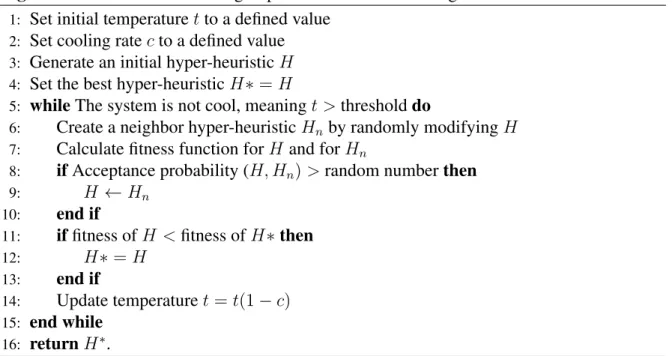
(31) CHAPTER 2. THEORETICAL FRAMEWORK. 18. of a previous work of Burke et al. [22] similar to the work also described in the previous paragraph [23], but instead of using tabu search, they combine that approach with a simulated annealing framework. Another notable example of perturbative approaches reviewed by Burke et al. [21] is the work by Ropke et al. [98], where the authors study the pickup and delivery problem for constructing routes. In this case, the hyper-heuristic involves an adaptive method for choosing heuristics based on historical performance, and furtherly updating each of the heuristics’ performance during the solution process.. 2.4.2. Other High-level Methods. Most of the approaches used to produce hyper-heuristics involve the use of a search strategy that relies on either in genetic algorithms or a variation of them, or other search-based meta-heuristics such as simulated annealing and tabu search. However, recent trends [93, 21] include the exploration of other strategies. For example, Sabar et al. [100] construct a tree of low-level heuristics and perform Monte Carlo tree search to identify the sequences of heuristics to be applied. Another one is the work by Kheiri and Keedwell [64]. In this case, instead of using a search strategy, they produce a Markov model to assert the performance of sequences of heuristics to solve the optimization problems. Although this is not a search strategy by itself, it illustrates how other trends of research in the area of hyper-heuristics have arisen.. 2.5. Simulated Annealing. In the proposed solution model, the HH is trained with a Simulated Annealing process. This metaheuristic, originally presented by Kirkpatrick, Gelatt and Vecchi [65], is one of the simplest and most general techniques which turned out to be one of the most efficient ones. The algorithm mimics the crystallization process during cooling or annealing: when the material is hot, the particles have high kinetic energy and move more or less randomly regardless of their and the other particles’ positions. The cooler the material gets, however, the more the particles are “torn” towards the direction that minimizes the energy balance. The SA algorithm does the same when searching for the optimal values for the decision parameters: it repeatedly suggests random modifications to the current solution, but progressively keeps only those that improve the current situation. SA applies a probabilistic rule to decide whether the new solution replaces the current one or not. This rule considers the change in the objective function (measuring the improvement/impairment) and an equivalent to “temperature” (reflecting the progress in the iterations). Dueck and Scheuer [39] produced a variation of the algorithm by suggesting a deterministic acceptance rule instead which makes the algorithm even simpler: accept any random modification unless the resulting impairment exceeds a certain threshold; this threshold is lowered over the iterations. This variation is known as Threshold Accepting (TA). The pseudocode of the complete SA algorithm is due to Maringer [81] and shown in Algorithm 1. There are several parameters of the SA algorithm that can be adjusted. A notable one is the cooling schedule, that is, the procedure by which the temperature is updated. The most used is the traditional one defined by Kirkpatrick et al. [65] which is shown in Equation 2.2. However there are other approaches in the literature [79], such as a logarithmic cooling.