Modelling of sectoral energy demand through energy intensities in MEDEAS integrated assessment model

Texto completo

(1)Energy Strategy Reviews 26 (2019) 100419. Contents lists available at ScienceDirect. Energy Strategy Reviews journal homepage: http://www.elsevier.com/locate/esr. Modelling of sectoral energy demand through energy intensities in MEDEAS integrated assessment model ~ igo Capell�an-P�erez a, b Ignacio de Blas a, *, Luis Javier Miguel a, b, In a b. Research Group on Energy, Economy and System Dynamics, Escuela de Ingenierías Industriales, Paseo del Cauce s/n, University of Valladolid, 47011, Valladolid, Spain Systems Engineering and Automatic Control, Escuela de Ingenierías Industriales, Paseo del Cauce s/n, University of Valladolid, 47011, Valladolid, Spain. A R T I C L E I N F O. A B S T R A C T. Keywords: Integrated assessment modelling Energy intensity Energy demand Technological change Electrification. The estimation of future energy demand is a key factor for the development of effective alternative policies towards a low carbon economy. This paper describes a novel method to estimate the energy demand in the new integrated assessment framework MEDEAS based on the projection of sectoral final energy intensities. The dy namic of each of the sectoral final energy intensity is broken down into (1) improvement in energy efficiency and (2) substitution of the final energy. The speed of changes in these factors depend on physical supply-demand unbalances in the market, climate mitigation and other energy saving policies and the perception of scarcity of the different economic agents. The simulated case studies in MEDEAS-World under the narrative of the Business-as-usual (BAU) scenario have allowed validating the model’s robustness and showing the potentiality of its application.. 1. Introduction The global energy system has to change radically in the next few decades in order to deal with the double pressing challenges of fossil fuel depletion and global environmental change [1–4]. Analyses exploring pathways for the transition to achieve a low carbon economy typically apply modelling forecasting tools to design alternatives to current un sustainable trends [5–7]. A wide range of models exists depending on the level of integration between human and natural systems, from “en ergy models” focusing on energy systems to “Integrated Assessment Models” (IAMs) with a broader focus on the environ ment/economy/society systems and interlinks. The diversity of models in the literature is due to the different approaches used by modellers striving to capture the involved complex interactions and high un certainties [6,8,9]. The robust estimation of future energy demand is a key factor for the development of effective alternative policies, considering also the strong link between energy use and development in industrial societies [10, 11]. However, the estimation of future energy demand is very complex. and subject to uncertainties, depending on a diversity of factors: tech nological evolution, socio-cultural behavior, energy affordability, techno-sustainable potentials of energy resources, policies to be enforced, etc. [12,13]. Two main approaches are used in the literature for the estimation of future energy demand: (1) through the modelling of bottom-up, detailed demand for end-use services (e.g., passenger per km, freight per km; m2 of buildings, etc.); and (2) top-down through the projection of general trends at sectoral level applying econometrics to time series of aggregated indicators such as GDPpc, population, energy intensities or prices. Each method presents different pros and cons and are more suitable depending on the scope and aims of the overall modelling framework. The bottom-up approach is more precise and al lows to test more specific policies, but at a cost of subjectivity in system boundaries, time intensiveness, eventual lack of data and failing to capture market failures or system-responses such as the rebound effect or leakage effects. On the other hand, the top-down approach is more comprehensive and allows economy-wide analysis at the cost of missing the detail and relying on financial data [14,15]. As a consequence, bottom-up models tend to suggest that efforts to substitute away from. Abbreviations: BAU, Business-as-usual: CC; Climate change: EI, Energy intensity: EROI; Energy return on energy investment: FE, Final energy: FF; Forgetting factor: GDPpc: Gross domestic product per capita: GG, Green growth: GHG; Greenhouse gas: IAM, Integrated assessment model: IEA; International Energy Agency: IOA, Input output analysis: NRE; Non-renewable energy sources: O&M, Operation and maintenance: PS; Perception of scarcity: RES, Renewable energy sources: RTS; Reference technology scenario: R&D, Research and Development: SS; Sensitivity to scarcity: TFEC, Total final energy consumption: WEO; World Energy Output: WIOD, World Input-Output Database. * Corresponding author. E-mail address: [email protected] (I. de Blas). https://doi.org/10.1016/j.esr.2019.100419 Received 30 September 2018; Received in revised form 5 July 2019; Accepted 8 October 2019 Available online 6 November 2019 2211-467X/© 2019 Elsevier Ltd. This is an open access article under the CC BY-NC-ND license (http://creativecommons.org/licenses/by-nc-nd/4.0/)..

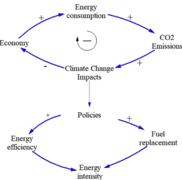
(2) I. de Blas et al.. Energy Strategy Reviews 26 (2019) 100419. Fig. 1. MEDEAS-W model schematic overview. Source: adaptation from Capell� an-P�erez et al. (2017a). The main variables connecting the different modules are represented by arrows. CC: climate change; EROI: Energy return on energy investment. *The climate change damage function can be specified by the user as a damage function or as an energy losses function.. specific forms of energy or to reduce greenhouse gas emissions would be easier than generally top-down models do [16]. GCAM [17], POLES-JCR [18], IMAGE-TIMER [19] or AIM [20] are examples of established models applying the first method, while MESSAGE [21,22], REMIND [23], WITCH [24], En-ROADS [25] or WEM [26] are examples of the second method, although a certain level of hybridization between both approaches also exists [16]. Energy intensity stands as a relevant indicator of energy efficiency in the literature, having a clear and intuitive definition and straightforward computation in models. This is despite the fact of being rather a broad concept with a high level of aggregation, which may mask the effect of eventual structural changes in the economy not related with efficiency improvements. In fact, the concept of energy efficiency was based on thermodynamic concepts [27]. As a consequence, alternative methods to measure energy efficiency such as a stochastic boundary approach [28], a distance function approach [29,30], or the innovative account ing framework of the energy end-use matrix [31] have been applied in the literature. Still, the energy intensity has been analysed as a key driver to guide the pathway of energy transition to achieve a low carbon economy [32–34]. Different types of energy intensity metrics exist depending on the energy and economic indicators used. Energy consumption can be measured in primary or final terms, and total or by disaggregating into different types of energy sources. Economic output can also be measured at sectoral or aggregated levels, GDP being one of the most frequent [5, 15]. A reduction in energy intensity over time indicates that the society uses less energy to produce the same value of goods of services, hence it implies a positive change that could also entail a sustainability improvement in the case of driving absolute decoupling between. resource use and economic activity [35]. Examples of models using projections of energy intensities to estimate future energy demand are MESSAGE [21,22], REMIND [23], EN-Roads [25] or WITCH [24]. However, the use of energy intensities for the estimation of future energy demand has shown also to have shortcomings. For example, Stern found that the energy intensity projections in the WEO reports since 1994 were overestimates of the actual improvement of energy intensity, which could be caused by a less effective implementation of energy efficiency policies as previously thought, and/or to the under estimation of the rebound effect in the economy [36]. Kaya show that the common use of constant elasticity of substitution functions for en ergy modelling in general equilibrium IAMs is problematic for the rep resentation of technology shifts [37]. In fact, virtually all models in the literature consider prices as a relevant indicator of scarcity. How to measure the scarcity or abundancy of natural resources has been a controversial issue in economics for a long time [38]. Ecological eco nomics criticizes the mainstream approach considering prices as a reli able indicator of scarcity of natural resources, given its theoretical and empirical weaknesses. Energy and mineral prices are subject to multiple influences (institutional framework, oligopolistic market structure, etc.), which prevent perfect competition to happen neither in the short nor long-term [39,40]. Moreover, given the inertia and rigidities in the productive processes highly dependent on natural resources, important adjustments in the economic system are produced via quantity changes (instead of prices), as post-Keynesian approaches have highlighted [41]. This paper describes and tests the approach followed to estimate the energy demand in the new integrated assessment framework MEDEAS which focuses on the biophysical and economic dimensions and in teractions arising during energy transitions [42]. Given the scope and 2.

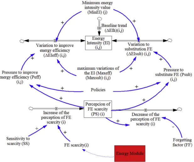
(3) I. de Blas et al.. Energy Strategy Reviews 26 (2019) 100419. sectoral-rich input-output structure with 35 economic sectors and households, a novel method based on the evolution of sectoral final energy intensities has been developed. Hence, energy demands are by-default modelled applying the top-down approach although it also allows for specific sectors to be modelled bottom-up. Input-output analysis lies on a matrix describing the past monetary flows between different industries. Its combination with satellite environmental ac counts allows to allocate the specific final energy consumption per unit of monetary output in each sector, attaining a high disaggregation at sectoral and final energy level. As input-output tables are static, system dynamics allow us to model economic behavior [43] and connect it to the rest of the MEDEAS submodules. System dynamics is a perspective and set of conceptual tools that enable us to understand the structure and dynamics of complex systems, as well as a modelling method that enables us to build formal computer simulations of complex systems [44, 45]. The integration of both approaches (IOA and system dynamics) has been identified as a promising avenue in the emerging field of macro-ecological modelling [43]. Additionally, given the aforemen tioned limitations of modelling prices as scarcity indicators, the devel oped MEDEAS model applies an alternative biophysical perspective to model final energy replacement which takes into account the evolution of the extraction of natural resources and their physical availability/ scarcity [46–48], as well as biophysical and thermodynamic limits in the substitution of inputs in production in the medium and long-term [49–51]. Availability and scarcity driving final energy shifts have been modelled in a flexible and transparent manner, avoiding fixed built-in optimization structures and black-box structures [52,53]. This paper is organized as follows: Section 2 explain briefly the MEDEAS framework and the role of the energy intensities, Section 3 explain the methodology followed to estimate the dynamic evolution of sectoral final energy intensities. Section 4 show and discuss the poten tialities of the method described in methodology section thought different sensitivity analyses and Section 5 outlines our conclusions.. Fig. 2. Causal loop diagrams representing the effects of final energy (FE) scarcity (a) and abundance (b) of a given final energy (i) in MEDEAS frame work. J represents WIOD economic sectors: 1 … 35 þ households.. 2. Short overview of MEDEAS framework. � Energy availability: this module includes the potential and avail ability of renewable energy sources (RES) and non-renewable energy resources (NRE), taking into account biophysical and temporal constraints. In particular, the availability of non-renewable energy resources depends on both stock and flow constraints [3,46,60]. In total, 25 energy sources and technologies, and 5 final energies are considered (electricity, heat, solids, gases and liquids), with large technological disaggregation. The intermittency of RES is considered in the framework, computing endogenous levels of overcapacities, storage and overgrids, depending on the penetration of variable RES technologies. This sub-module is mainly based on the previous model WoLiM [1]. Transportation is modelled in great detail, differenti ating between different types of vehicles for households, as well as freight and passenger inland transport (see Ref. [42] for details). � Energy infrastructures & EROI: This module represents power plants to generate electricity and heat, allowing planning and construction delays to be considered. A net energy approach is applied [61] endogenously and dynamically accounting for the Energy Return on Energy Investment (EROI) of both individual technologies and the EROI of the system. The demand of energy is affected by the varia tion of the EROI of the system. � Materials: materials are required by the economy, with emphasis on those required for the construction and O&M of alternative energy technologies [62]. Recycling policies are available. � Land-use: currently, this module mainly accounts for the land re quirements of the RES energies. � Water: this module allows calculating water use by type (blue, green and gray) by economic sector and for households. � Climate (only in MEDEAS-W): this module projects the climate change levels due to the GHG emissions generated by human. MEDEAS is a set of a policy-simulation dynamic-recursive models at three different geographical scales following the same conceptual approach: global one-region [42], EU [54] and country-level [55]. These models have been designed applying System Dynamics,1 which facili tates the integration of knowledge from different perspectives and dis ciplines as well as the feedbacks from different subsystems. The models typically run from 1995 to 2060 (although the simulation horizon may be extended to 2100 if necessary, e.g. when focusing on climate change issues). The models are structured in eight main sub-modules: Economy, Energy, Infrastructures, Materials, Land Use, Water, Climate and Social & Environmental Impact Indicators. The main characteristics of each module in MEDEAS framework are: � Economy and population: the global economy is modelled assuming non-clearing markets (i.e., not forcing general equilibrium), demand-led growth and complementarity instead of perfect substi tutability. Hence, production is determined by final demand and economic structure, combined with supply-side constraints such as energy availability. The economic structure is captured by the adaptation and dynamic integration of global WIOD input-output tables, resulting in 35 industries and 4 institutional sectors [56]. Final energy intensities by sector are obtained by combining infor mation from the WIOD environmental accounts [57] and the IEA Balances [58]. Population evolves exogenously as defined by the user. See Ref. [59] for more details on this sub-module.. 1 Developed in Vensim DSS software for Windows Version 6.4E (x32). Also available in Python open-source code (http://www.medeas.eu/).. 3.

(4) I. de Blas et al.. Energy Strategy Reviews 26 (2019) 100419. intensities by sector. It is assumed that the relative scarcity of a type of final energy favors its replacement. When, in a sector, there is a sub stitution of one type of final energy by another, a substitution of their corresponding energy intensities is also produced. (see Fig. 2 and section 3 for specific definitions applied). Fig. 2a represents the situation when a given final energy i is more scarce than other final energies, driving its replacement, while Fig. 2b represents the opposite situation, i.e., final energy i is more abundant and tends to replace other final energies. As represented in Fig. 2a, three feedback loops tend to stabilize the system when there is scarcity for a given final energy. Economic growth tends to increase the consumption of energy and therefore increases the possibility of scarcity of that final energy. In turn, this scarcity can slow down the economy (L 1). On the other hand, the scarcity of a final energy drives the effort to improve energy efficiency in the consumption of such final energy. This reduces its energy intensity and consequently reduces energy consumption (L 3). Likewise, the scarcity of one type of final energy drives its replacement by another that is more abundant. This reduces the energy intensity of the replaced final energy increasing accordingly the energy intensity of the final energy which replaces it. If the energy intensity is reduced, it will also reduce energy consumption (L 2). In the case of more abundant or less scarce energy types, the two loops also stabilize the system, but in a different way (Fig. 2b). The in crease in consumption decreases the abundance of the resource. Abun dance increases the chances of this final energy to be used to replace other, scarcer final energies, and as a result, its energy intensity in creases. In both cases, the key role of energy intensity in the MEDEAS framework is observed. The most detailed modelling of energy intensity, which is the main objective of this paper will be described in section 3. In the previous casual loop diagrams, the substitution of a final en ergy has been related only to scarcity, but nowadays, the substitution of fossil fuels is also motivated by policies, especially climate change mitigation policies (e.g., Paris Agreement [67]). Fig. 3 shows the global basic relationships between energy economy and climate change in the MEDEAS framework. The impacts of climate change affect the socioeconomic dimensions motivating the enforce ment of climate change mitigation policies such as a greater effort for energy efficiency and the substitution of fossil fuels by renewable en ergies, which is ultimately related with energy intensities. Therefore, changes in energy intensity will be driven by two processes: (a) changes in energy efficiency and (b) replacement in the final energy type used in each industrial sector. In the next section, dedicated to describe the applied methodology, the focus will be on disaggregating these two processes.. Fig. 3. Causal diagram representing the effect of climate change-motivated policies on energy intensity in MEDEAS framework.. societies (non-CO2 emissions are exogenously set, taking RCPs sce narios as reference [63]). The carbon and climate cycle is adapted from C-ROADS [64,65]. This module includes a damage function which translates increasing climate change levels into damages for the human systems [66]. � Social and environmental impacts: this module translates the “bio physical” results of the simulations into metrics related with social and environmental impacts. The objective of this module is to contextualize the implications for human societies in terms of wellbeing for each simulation. In this work, MEDEAS-World (MEDEAS-W) is used for illustrating the developed method for estimating sectoral final energy demands. Fig. 1 shows the conceptual schematic overview of the different modules. The model dynamically operates as follows. For each period: first, a sectoral economic demand is estimated from an exogenous and dynamic GDPpc objective. The demand of final energy required to meet pro duction is obtained using energy-economy hybrid Input-Output Anal ysis, and combining monetary output and energy intensities by final energy sources. Second, the energy sub-module computes the net available final energy supply, which may satisfy (or not) the required demand: the economy adapts to eventual scarcity of final energy. Third, materials required to build, operate, maintain, dismantle, etc., are estimated. This allows the EROI of the system to be estimated as well as eventual material bottlenecks to be assessed (although material avail ability does not constrain economic output in the current model version). Fourth, the climate sub-module computes the GHG emissions, whose accumulation derives in a certain level of climate change, which in turn feeds back to the economic sectoral output. Additional land and water requirements are accounted for. Finally, the social and environ mental impacts are computed.. 3. Methodology This section describes the methodology developed to estimate the sectoral final energy demand in MEDEAS models. The top-down approach is more practical with high sectoral disaggregation, which is the case of MEDEAS framework with 35 economic sectors and house holds, and allows for economy-wide analysis at the cost of missing the detail of particular sectors [14,15]. Hence, a novel method based on the top-down projection of the evolution of sectoral final energy intensities has been developed. By multiplying the the sectoral and houselholds final energy intensities by the sectoral production and the households demand, we obtain the estimation of the total final energy demand by final energy required to produce the economic output. Energy demands are by-default modelled applying the top-down approach, although MEDEAS modelling approach also allows for specific sectors to be modelled bottom-up, which has in fact already been performed for inland transport sector (see Ref. [42]). In this paper a top-down approach for all the sectors has been applied for the sake of simplicity. Input-output analysis lies on a matrix describing the past monetary flows between different industries. Its combination with satellite environ mental accounts allows to allocate the specific final energy consumption per unit of monetary output in each sector.. 2.1. Energy intensities in MEDEAS framework MEDEAS models contain several feedbacks between variables of different modules. Energy intensity plays a key role in the feedback between economic variables (output and demand) and the availability of energy resources. Five types of final energy are considered (electricity, heat, solids, gases and liquids), which give rise to 5 final energy 4.

(5) I. de Blas et al.. Energy Strategy Reviews 26 (2019) 100419. MEDEAS framework considers 5 types of final energy consumption (i:1 … 5: electricity, solids, liquids, gases and heat) and 35 economic sectors (j:1 … 35 according to the WIOD classification) [56,57,68]. In addition, the energy intensity of households is calculated as the ratio between each of the final energy types and their total consumption in economic terms (Eq. (2)). Consequently, a total of 180 (36 � 5) final energy in tensities are obtained in MEDEAS framework.. MEDEAS framework has been implemented in models at three different geographical scales: global one-region [42], EU [54] and country-level [55]. The specific parametrization for MEDEAS-W model is described in section 3.4. Section 4 shows and discusses the results of 4 case studies simulated with MEDEAS-W to illustrate the potentialities of the method. The application of global sectoral final energy intensities in MEDEAS-W allows to properly represent global energy consumption trends whose modelling at EU or country-level may introduce biases. In particular, structural changes in many western countries recently have tended to reduce the production of heavy industry products and increase their imports from emerging countries [10].. Final households energy intensity ¼. Final energy intensity ¼. Households final energy consumption by type of energy Households economic consumption. 3.1. Baseline trend. Final energy by sector and type of final energy Total output by sector. 1. 2. The starting point for modelling the dynamic behavior of final en ergy intensities is the available historical data. These data have been taken from WIOD database environmental accounts [57], which have a time horizon from 1995 to 2009. However, calculations had to be per formed applying data from the IEA balances to correct the double ac counting from WIOD database to use appropriately the energy intensities in MEDEAS framework. It is important to remark that WIOD database assign the energy consumption of private vehicles to. As aforementioned, energy intensity usually expresses a ratio be tween the energy used in a process and its economic output. In this way, the energy intensity is a highly aggregated indicator. However, the same concept can be applied at sectoral level [15] (Eq. (1)) ratio between final energy by sector and type of final energy and total output by sector which is the total value of all goods and services produced in a sector. With the objective of disaggregating final energy intensities, the. Fig. 4. Causal loop diagram representing the main features of the modelling of energy intensities in MEDEAS framework. FE scarcity can eventually also be affected by climate change damages in the case of applying a energy losses damage function. I represents final energy. J represents WIOD economic sectors: 1 … 35 þ households. 5.

(6) I. de Blas et al.. Energy Strategy Reviews 26 (2019) 100419. households sector, as opposed to other databases that assign this energy to the transport sector. Based on this historical data, the first component that explains the behavior of energy intensities in MEDEAS framework is defined as the baseline trend. This baseline trend can be considered the stationary component of the dynamic evolution of final energy intensity and is obtained as the average value of the annual relative variation of the. can accelerate changes in energy intensity and are represented in Fig. 4 as “Policies”. These factors that affect the variations of the energy intensity (ΔEIeffij and ΔEIsubij) acting as a pressure to improve the energy efficiency (Peffij see eq. (5)) and to change the final energy (Psubij see eq. (6)). Peffij and Psubij range 0–100% depending on the implementation speed of the policy and the effects of the scarcity. In policies, the model user can set the initial and target year (when the pressure attains the 100%), as well as select 3 different implementation speeds (slow, medium, rapid) depending on the setting of the exogenous policy.. available data ðΔEIhij Þ. Following the proposal of [69], the inertial ten. dency of the energy intensity is shown in Eq. (3) for each sector (i) and final energy (j). The estimated values of ΔEIhij are shown in Table A. 1 Appendix A. If ΔEIhij > 1, a linear regression is applied. EIij ðtÞ ¼ ΔEIhij ⋅EIij ðt. (3). 1Þ. On top of the baseline historic trend, variations can be applied as a consequence of different assumptions to be applied in simulated scenarios.. In the energy transition towards a low carbon economy, energy in tensity (EIij) is assumed that changes by: a) Variation (relative change) in the energy intensity due to the improvement in energy efficiency, associated with the technology used in the consumption of each type of final energy and sector (ΔEIeffij). Historically, energy intensity has tended to decrease due to technological improvements in energy efficiency. This tendency has been traditionally represented in IAMs as Autonomous Energy Effi ciency Improvement (AEEI) [19,20,70,71]. The estimates for this decrease due to the AEEI vary between 0.5% and 2% per year in the literature [70]. Here, the historical data from the WIOD database [57] are taken as reference. b) Variation (relative change) in energy intensity due to the substitution of one type of final energy by another (ΔEIsubij). In this case, the type of energy that is replaced decreases its final energy intensity and the type of energy that replaces the previous one increases its final en ergy intensity. These variations will have opposite signs and may be different in absolute value depending on differences on the energy efficiency of each technology linked to the type of final energy used. In this case, it is necessary to bear in mind that these changes in the type of final energy used in each sector require significant in vestments in equipment and technology, so that their speed will be limited.. The variations of the sectoral final energy intensities ΔEIsubij) are assumed to be driven by two main factors:. Psub ij ¼ Effects of scarcity þ Effects of policies. 6. ΔEI eff ij ¼ Peff ij *Maxeff ij. 7. ΔEI sub ij ¼ Psub ij *Maxsub ij. 8. Mathematically, EIjj could converge to zero in a sufficiently long time. However, any process requires energy, and there are biophysical and thermodynamic limits in the substitution of inputs in production in the medium and long-term [49–51]. Although technological learning tends to improve energy efficiency, improvement rates tend to decrease over time when the technology reaches a certain degree of maturity (decreasing marginal returns). As a whole, this would mean that the energy intensity for each economic sector could reach a minimum value, that should be above zero. Consequently, the variation rates of the en ergy intensity can suffer a deceleration when it approaches this mini mum (MinEIj) (see section 3.4.b) for the setting of exogenous parameters).. Hence, the resulting variation of EIij is shown in Eq. (4). The pro posed method disaggregates these two variations as flows and the en ergy intensity as stock as can be seen in Fig. 4. (4) (ΔEIeffij. 5. As a first approximation, the model assumes by-default that future variations of sectoral final energy intensities will be within the ranges of variations that have occurred in the past. Although it is possible that in the future these variations could exceed those that occurred in the his torical data series available, it is important to point out two aspects. On the one hand, the viability of variations in energy intensity is subject to technological and socioeconomic limitations, so that the maximum annual variations must be limited in any case. On the other hand, the fact that there has been a maximum variation in a given year does not necessarily prove that this variation can be maintained over time. Therefore, an estimate of the maximum variations of the energy in tensities (Maxeffij and Maxsubij) has been obtained from historical data. In any case, these generic statistical estimates (see section 3.4) can be specified by the model user based on specific knowledge on the energy intensity of each sector and type of final energy and the technologies involved (see Fig. 4). Equations (7) and (8) show how the variations of sectoral final energy intensities due to efficiency improvements and final energy substitutions, respectively, are obtained. When the pressure at tains 100%, these variations correspond with the respective maximums.. 3.2. Variations over the baseline trend. sub ΔEIij ¼ ΔEIhij þ ΔEI eff ij þ ΔEI ij. Peff ij ¼ Effects of scarcity þ Effects of policies. 3.3. Scarcity of a type of final energy and its perception. and. Given the aforementioned limitations of modelling prices as scarcity indicators [39–41], MEDEAS framework applies a biophysical perspec tive to model final energy replacement which takes into account the evolution of the extraction of natural resources and their physical availability/scarcity [46–48]. The scarcity and/or abundance of a final energy is obtained in the energy module based on the relationship between the annual demand and supply of each type of final energy consumed (see Eqs. (9) and (10)).. a) Market factors related to the scarcity of each type of energy. The scarcity of a type of energy can lead to greater efforts to increase energy savings and improve efficiency, as well as the substitution of that type of energy by more abundant ones. Indicators of physical scarcity have been specifically developed in order to represent physical supply-demand unbalances. Market factors are modelled through the variable “Perception of final energy scarcity” (PSi) (see Fig. 4). b) Sociopolitical factors. Some policy measures, such as climate change mitigation policies, are promoting a greater effort in energy effi ciency and fostering the substitution of fossil fuels. These measures. scarcityi ¼ 1. abundancei. abundancei ¼ 1 6. demandi supplyi demandi. 9 10.

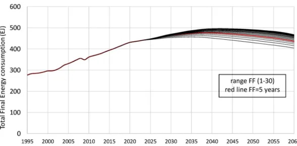
(7) I. de Blas et al.. Energy Strategy Reviews 26 (2019) 100419. When the demand of a given final energy is fulfilled, the scarcity is zero, being >0 when the supply cannot fulfill the demand. In order to model the effect of the scarcity of each type of final energy on the energy mix, a variable called perception of the scarcity (PSi) has been defined. This variable increases with the annual scarcity of each type of energy and decreases with time. The impact caused by novel situations, such as terrorist attacks or abrupt price rises, provokes rapid socioeconomic reactions, but their effects dissipates over time if new information on the same subject is not received [72]. In the case of final energy scarcities, steeper energy price increases or news in the media can have an effect. Although the behavior of social and economic agents may vary (companies and final consumers), the PSi has been chosen in order to model this behavior. Hence, the PSi increases with the annual situations of scarcity and diminishes over time. Forgetting Factor (FF) represents the time over which past periods of energy scarcity are forgotten and then do not drive final energy replacement any more. FF is a parameter widely used in adaptive control algorithms in different areas, such as [73,74]. In order to take into consideration that depending on the context and scenario, different perceptions to scarcity may exist, i.e., more or less propensity to improve efficiencies and final energy replacement for the same scarcity levels, the variable Sensitivity to Scarcity (SS) is introduced and it can be defined by the user. Eq (11) represents how PSi is obtained (see Fig. 4). PSi ðtÞ ¼ scarcityi *SS þ PSi ðt. 1Þ=FF. � sub Maxsub ij ¼ μ ΔEIij. 3.4.3. Calibration of the forgetting factor (FF) As aforementioned, FF represents the time over which past periods of energy scarcity are forgotten. Uncertainty analysis has been applied to calibrate this factor, performing simulations with FF ranging from 1 to 30 years (see results in Figure B. 1 of Appendix B). The results show in total final energy consumption (TFEC) that median value is five years, then by default FF in the model is five.. 11. Table 1 Cases simulated in this work. FE: final energy; PS: perception to scarcity; Maxeffj: annual maximum efficiency improvement; Maxsubij: annual maximum of sub stitution of one type of final energy by another. Name of simulations. 3.4.1. Estimation of maximum variations of the final energy intensities (Maxeffij and Maxsubij) The estimation of maximum annual variations of the final energy intensities (Maxeffij and Maxsubij) is based on the matrices of final energy intensities EIij for the years 1995–2009 of WIOD database [57]. The annual final energy intensities have been obtained for each sector as well as the variations of both (ΔEIhij). In order to be able to disaggregate the energy intensity variations due to (1) the efficiency improvement (ΔEIh eff h sub ij) and (2) the substitution of the final energy type (ΔEI ij), it has been assumed that, within each economic sector, the reduction in energy intensity of each type of replaced energy in regard to sector energy in tensity variation (ΔEIhj) is compensated by the decrease in the other type of energy that replaces the previous one (see eq. (12)). 12. Therefore,. h ΔEIsub ij ¼ ΔEI ij. 13 14. ΔEI hij eff (ΔEIh effij. Description of simulations. Case 1: Final energy replacement No_Rep FE replacement not activated Rep_L FE replacement with Low PS Rep_M FE replacement with Medium PS Rep_H FE replacement with High PS Rep_L_unL FE replacement with Low PS and unconstrained gas and coal supply Rep_M_unL FE replacement with Medium PS and unconstrained gas and coal supply Rep_H_unL FE replacement with High PS and unconstrained gas and coal supply Case 2: Final energy replacement þ exogenous efficiency improvement Rep_M Ref MaxEff FE replacement with Medium PS and reference Maxeffj estimated in section 4.3 Rep_M 50% FE replacement with Medium PS and Maxeffj 50% less than MaxEff reference Maxeffj Rep_M 25% FE replacement with Medium PS and Maxeffj 25% less than MaxEff reference Maxeffj Rep_M 25% MaxEff FE replacement with Medium PS and Maxeffj 25% more than reference Maxeffj Rep_M 50% MaxEff FE replacement with Medium PS and Maxeffj 50% more than reference Maxeffj Case 3: Final energy replacement þ electrification of households Rep_M Ref MaxSub FE replacement with Medium PS and reference Maxsubij estimated in section 4.3 Rep_M 50% FE replacement with Medium PS and Maxsubij 50% less than MaxSub reference MaxSubij Rep_M 25% FE replacement with Medium PS and Maxsubij 25% less than MaxSub reference MaxSubij Rep_M 25% FE replacement with Medium PS and Maxsubij 25% more than MaxSub reference MaxSubij Rep_M 50% FE replacement with Medium PS and Maxsubij 50% more than MaxSub reference MaxSubij Case 4: Final energy replacement þ exogenous efficiency improvement þ electrification of households Rep_M All Pol FE replacement with Medium PS and Maxeffj and Maxsubij estimated section 4.3. i¼1. ΔEI hij eff ¼ ΔEI hj. 16. 3.4.2. Selection of minimum value in final energy intensity (MinEIij) As aforementioned, biophysical and thermodynamic limits affect the substitution of inputs in production in the medium and long-term [49–51]. However, where this limit stands for each sector is subject to large uncertainties. For the sake of simplicity, a common value for all sectors is set at 30% of the level of 2009 taking as reference the study of Lightfoot and Green [75]. This study analyzes the potential efficiency improvements for different sectors (electricity, transportation, residen tial, industrial and commercial) until 2100 considering potential tech nical energy efficiency improvements globally (both by inventing and implementing new technology and by implementing most current effi cient technologies).. The exogenous parameters of the model can be adjusted basing on expert knowledge on each sector and type of final energy. Here, we describe how the by-default values included in the MEDEAS-W model have been estimated taking available historical data as reference.. � ΔEI hj � 0. vffiffiffiffiffi�ffiffiffiffiffiffiffiffiffiffiffiffiffiffiffi�ffiffi u uσ 2 ΔEIsub ij t þ n*ð1 αÞ. where the confidence interval (α) is 90%.. 3.4. Estimation of the exogenous parameters of the model. 5 � X ΔEI hij eff. �. h sub. The variables y ΔEI ij) (see eqs. (13) and (14)) are modelled as random variables with a probability distribution defined by their mean value and their variance: μ((ΔEIh effij), σ2(ΔEIh effij) y μ(ΔEIh sub 2 h sub ij). ij), σ (ΔEI The maximum values (eqs. (15) and (16)) used in the model depends on these mean value and variance for a given confidence interval and are shown in Table A. 2 and Table A. 3 of Appendix A. sffiffiffiffiffiffiffiffiffiffiffiffiffiffiffiffiffiffi�ffiffi σ 2 ΔEIeff j eff Maxj ¼ 15 n*ð1 αÞ 7.

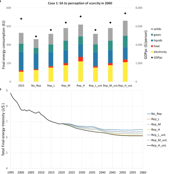
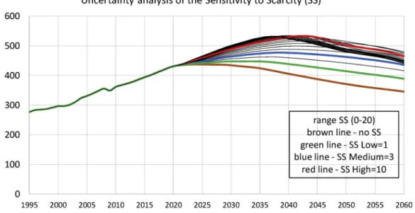
(8) I. de Blas et al.. Energy Strategy Reviews 26 (2019) 100419. Fig. 5. Case 1: final energy replacement assuming different levels of perception to scarcity and availability of gas and coal. a) final energy consumption mix in the year 2060 for each simulation and comparison with the final energy consumption mix in 2015. Rhombuses represent the GDP per capita in 2060 measured in $ per capita. b) 2015–2060 evolution of the total final energy intensity in J/$ per simulation. Total final energy intensity is computed as TFEC/GDP. (Dollars correspond to 1995US $) The description of the simulations is shown in Table 1. See Table 1 for the nomenclature and description of each simulation.. 3.4.4. Calibration of the sensitivity to scarcity (SS) The value of this parameter depends on human behavior (e.g., cul tural context, enforced policies, etc.) and the dynamics of the energy system (e.g., resistance to change, lifetime of operating power centrals, vested interests in polluting businesses, etc.). Hence, in MEDEAS this parameter is scenario-dependent. To facilitate the use of the model, three default values have been calibrated, associated to Low, Medium and High sensitivity to scarcity, although any user can choose the value to use. For the calibration process, an uncertainty analysis of this parameter has been performed for a wide range of values (0–20). The results showed the highest value in TFEC corresponds to ten, then it is the high value of SS. Between the high value and the results of zero value, three similar ranges have been made to obtain Medium and Low values. The results of the uncertainty analysis are shown in Figure B. 2 of Appendix B. This variable has been calibrated as Low (SS ¼ 1), Medium (SS ¼ 3) y High (SS ¼ 10).. intensities proposed in this study within the MEDEAS-W model, an un certainty analysis has been carried out. The steps taken in this uncer tainty analysis were the following: 1. Identification of parameters affected by uncertainty. 2. Assessment of the conditional probability ranges associated with these parameters. 3. Use of Monte-Carlo sampling in MEDEAS-W to calculate uncertainty results n ¼ 100 Monte Carlo simulations are performed with the MEDEAS-W model considering 5 uncertainty inputs, Maxeffj, Maxsubij, MinEIj, FF y SS. The probability ranges of each variable are defined in Table B. 1 of Appendix B. A uniform distribution has been used for each variable. The results of uncertainty analysis represented in Figure B. 3 show the sta bility of the model (variations of more than �100% from the reference value in input parameters obtain variation of less than �15% in TFEC and less than �10% in total final energy intensity from the reference value).. 3.5. Uncertainty analysis of the exogenous parameters of the model In order to validate the method of evolution of final energy 8.

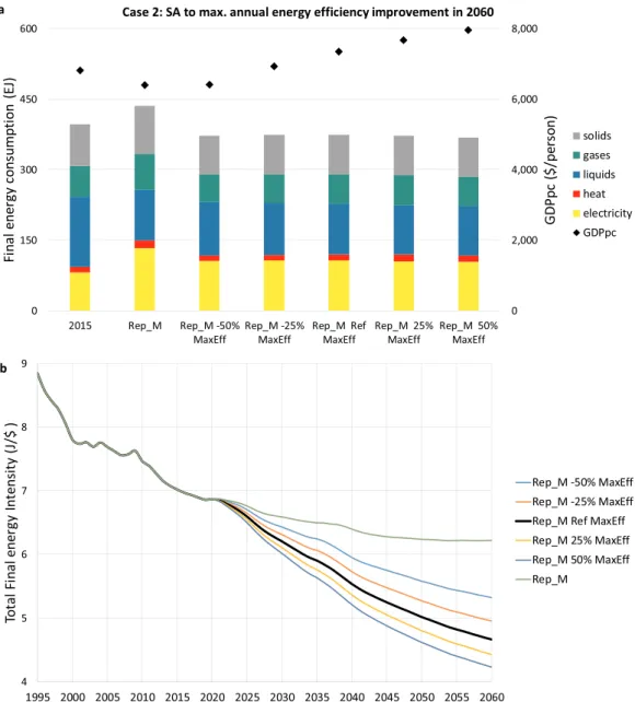
(9) I. de Blas et al.. Energy Strategy Reviews 26 (2019) 100419. 4. Results and discussion. this work.. This section shows the simulation of several experimental case studies based on a common business-as-usual (BAU) narrative. The objective of this section is to show the main potentialities of the devel oped method for modelling the sectoral energy demand in MEDEAS-W model. The BAU narrative represents the continuation of major cur rent trends and dynamics and is implemented within IAMs to be used as counterfactuals against which policy scenarios are developed [76,77]. For the specification of the BAU narrative through a consistent set of inputs, a varied and rich literature has been examined: scientific papers and technical documentation [3,56,59,68,78]; reports and databases from international/national agencies and organizations such as the In ternational Energy Agency, IRENA, the US Energy Information Admin istration or the UNEP [58,79–85]; industry prospect assessments [86] and analyst investors [87], which in some cases had to be complemented with own estimations. Appendix C and Table C. 1 depicts the description of the most rele vant inputs and assumptions which characterize the BAU narrative in. 4.1. Experimental case studies Three main features of the developed method are explored through four experimental case studies: final energy replacement driven by biophysical scarcity, exogenous energy efficiency improvement policy, electrification policy in households and finally a case combining all of them. Final energy replacement is by-default activated in all case studies. A total of 18 simulations cases have been run and are summa rized in Table 1: 4.1.1. Final energy replacement Fig. 5 shows the results of the sensitivity analysis carried out with different options affecting the FE replacement in MEDEAS-W. First, a simulation is run with the FE replacement deactivated (No_Rep). Sec ond, three simulations are run for three different levels of SS (Low, Medium, High) and named Rep_L, Rep_M and Rep_H, respectively. Third, three more simulations, one per SS level, are carried out assuming. Fig. 6. Case 2: Policy of energy efficiency improvement. a) final energy consumption mix in the year 2060 for each simulation and comparison with the final energy consumption mix in 2015. Rhombuses represent the GDP per capita in 2060 measured in $ per capita. b) 2015–2060 evolution of the total final energy intensity in J/ $ per simulation. The black thick line represents the simulation considering the values for Maxeffj estimated in section 3.4. Total final energy intensity is computed as TFEC/GDP. (The dollars correspond to 1995US $). See Table 1 for the nomenclature and description of each simulation. 9.

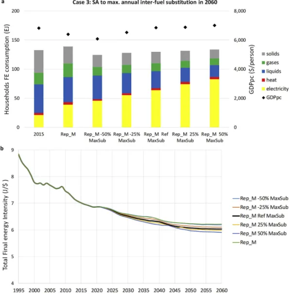
(10) I. de Blas et al.. Energy Strategy Reviews 26 (2019) 100419. that no relevant supply constraints to the availability of natural gas and coal exist during the analysis horizon. In fact, there is a large uncertainty with relation to the future availability of both fossil fuels (which is generally found to be larger than for oil [88]). A reduced fraction of unconventional gas -coal bed methane, hydrates, shale and tight gas-has only recently become economically profitable (e.g. shale oil and gas) and extraction techniques for some resources are still under research & development (R&D) (e.g. methane hydrates). As a result, few published estimates exist with large associated uncertainties [88–90]. Coal is usually seen as a vast abundant resource, although there are large un certainties related to the base of available resources due to the lack of robust global estimates [88,90,91]. Those three simulations are Rep_L_unL, Rep_M_unL and Rep_H_unL. Fig. 5a shows that in the simulation in which FE is deactivated, both the total final energy consumption (TFEC) and the global average GDPpc would be lower by 2060 than current levels, around 10% and 30% respectively. Population increase means that in per capita terms, the TFEC would fall by 50% in relation to current levels. When FE replacement is activated in the simulations, the perception of scarcity (PS) drives the shift of final energy intensities. The final en ergy intensities of those energy resources which are affected by scarcity. are reduced and those relatively more abundant increase accordingly. In this way, the TFEC and GDPpc in all cases with FE replacement activated are greater than when there is no FE replacement. As expected, the larger is the sensitivity to scarcity, the larger are the TFEC and GDPpc by 2060. This is due to the fact that greater substitution between final en ergies allow to satisfy a larger energy demand and the effects of scarcity are hence reduced. However, the relationship is found to be non-linear: higher availability of final energy translates into an even higher pro duction of added-value. However, only the simulation assuming high PS manages to maintain the same level of GDPpc by 2060 with relation to 2015 levels. Another trend common to all simulations relates to the progressive electrification of the system with increasing levels of PS. Electricity covers 25% when the FE replacement is deactivated, while reaching 35% in the case of high level of PS. This is due to the fact that renewable energy technologies for the generation of electricity are assumed to continue current high growth trends. A similar effect is found for heating due to the same phenomenon, but of smaller importance. Assuming that natural gas and coal resources are not constrained during the timeframe of the analysis, the results by 2060 do not signif icantly change for the low and medium PS in relation to the case where. Fig. 7. Case 3: Policy of electrification in Households sector. a) households final energy consumption mix in the year 2060 for each simulation and comparison with the final energy consumption mix in 2015. Rhombuses represent the GDP per capita in 2060 measured in $ per capita. b) 2015–2060 evolution of the total final energy intensity in J/$ per simulation. The black thick line represents the simulation considering the values for Maxsub estimated in section 3.4. Total final energy intensity is computed as TFEC/GDP. (The dollars correspond to 1995US $). See Table 1 for the nomenclature and description of each simulation. 10.

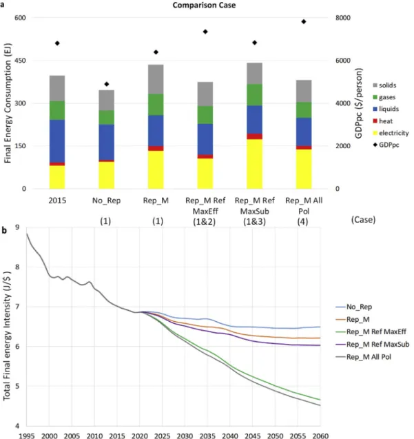
(11) I. de Blas et al.. Energy Strategy Reviews 26 (2019) 100419. they are constrained by maximum supply curves. This is due to the fact that the scarcity affecting these simulations is related to liquid fuels and there is no problem of scarcity in the energy resources of natural gas and coal. However, for the simulation assuming high PS, the TFEC and GDPpc are higher than in the constrained gas and coal availability simulation and the energy mix has also changed. In the simulation where all the fossil resources are limited, when replacing liquid resources (first resource in suffering scarcity) by gases and solids, there is a scarcity in the substitute resources preventing the increase in TFEC and therefore GDPpc. When natural gas and coal resources are not constrained, all liquid resources are replaced by gases and solids, which increases the TFEC. The final solid energy consumption in 2060 increases by 20% in the case of resources limited to 25% when the coal is not constrained during the timeframe of the analysis. Similar occurs in the case of gases, increasing by around 15%–20%. Fig. 6b shows the dynamic evolution of the total energy intensities in the different simulations. Differences between simulations are reduced, ranging 8–12% cumulated improvement from the year 2015 by 2060.. 4.1.2. Case 2: policy of energy efficiency improvement In this case study, different levels of exogenous improvement in energy efficiency are introduced into the model at both sectoral (35 economic sectors and households) and final energy level (5 final en ergies). The policy is set to start in 2020, the pressure of the policy (Peffij) reaching 100% of Maxeffj in 2060 (medium implementation speed). The policy of improving energy efficiency depends on the annual maximum efficiency improvement (Maxeffj) which has been estimated in section 3.4 for each sector and final energy. All the simulations in this case study have been carried out with FE replacement activated and sensitivity to scarcity with a Medium value, so they can be compared with the Rep_M simulation (In Rep_M there is no exogenous policy of energy efficiency improvement). In this case study, the simulation tak ing into account the values for Maxeffj estimated in section 3.4 (Rep_M Ref MaxEff) is considered as reference. A sensitivity analysis is also carried out varying these maximum values by sector and final energy by �50 and � 25%, resulting in the simulations: Rep_M 50% MaxEff, Rep_M 25% MaxEff, Rep_M 25% MaxEff and Rep_M 50% MaxEff (see Table 1). Fig. 6a shows the results obtained for the different assumptions on. Fig. 8. Comparison case. a) final energy consumption mix in the year 2060 for each simulation and comparison with the final energy consumption mix in 2015. Rhombuses represent the GDP per capita in 2060 measured in $ per capita. b) 2015–2060 evolution of the total final energy intensity in J/$ per simulation. Total final energy intensity is computed as TFEC/GDP. (The dollars correspond to 1995US $). See Table 1 for the nomenclature and description of each simulation. 11.

(12) I. de Blas et al.. Energy Strategy Reviews 26 (2019) 100419. Fig. 9. Final energy intensity mix by sector in Rep_M simulation in J/$. Total final energy intensity is computed as sectoral FEC/sectoral total output. (The dollars correspond to 1995US $). Energy consumption of private vehicles is assigned to households sector.. exogenous policy of energy efficiency improvement. Given that all the simulations have the same conditions for FE replacement, the energy mix by 2060 is rather homogenous for all the simulations. In the simu lation applying the Maxeffj estimated (Rep_M Ref MaxEff) the TFEC is reduced in 2060 more than 10% while the GDPpc increases by 10% compared to the simulation without the introduction of the policy of efficiency improvement (Rep_M). This implies, as seen in Fig. 6b, that the energy intensity by 2060 for the simulation with Maxeffj estimated (black thick line) is almost 25% lower than without efficiency improvement policy (green line). This behavior is explained because the globally improvement of energy efficiency implies that final energy demand is significantly reduced in all sectors and for all types of energy, reducing the energy scarcity events and allowing the GDPpc to grow more than in the pre vious case without the policy of energy efficiency improvements. The sensitivity analysis to the values of Maxeffj estimated in section 3.4, allows us to show that, as expected, the greater the maximums, the greater the GDPpc and the lower the TFEC in 2060. However, an in crease of 50% in the maximum annual values of improvement of energy efficiency with respect to the estimated values (Ref_MaxEff) implies an increase of less than 10% of GDPpc and a reduction of less than 2% of TEC with respect to estimated values. Likewise, a reduction of 50% of. the maximum values with respect to the estimated values implies a reduction around 10% in GDPpc and 2% in FEC. Fig. 6b shows that a wide range between simulations is found in final energy intensities (between 25 and 40% cumulated improvement from the year 2015 by 2060). 4.1.3. Policy of electrification in households sector A policy of electrification of the households sector is introduced into the MEDEAS-W model to show its ability to work at sectoral level. The substitution of the other final energies (excepting heat) by electricity causes the variation in the final energy intensities in households, which depends on the energy efficiency of each technology linked to the type of final energy used. For this case study, a saving of 50% of final energy has been assumed when replacing the solids, liquids and gases by electricity. This value is set taking as reference that some technological sub stitutions such as the electric car by internal combustion engine are estimated to represent savings of ~66% [42], while others such as heat generation from electricity would be <50%. The policy is set to start in 2020, the pressure of the policy (Psubij) reaching 100% of Maxsubij in 2060 (medium implementation speed). The policy of electrification in households sector depends on the annual maximum of substitution of one type of final energy by another 12.

(13) I. de Blas et al.. Energy Strategy Reviews 26 (2019) 100419. (Maxsubij) that have been estimated in section 3.4. All the simulations in this case study have been carried out with FE replacement activated and sensitivity to scarcity with a Medium value, so they can be compared with the Rep_M simulation (In Rep_M there is no exogenous policy of energy efficiency improvement). In this case study the simulation taking into account the values for Maxsubij estimated in section 3.4 (Rep_M Ref MaxSub) is considered as reference. A sensitivity analysis is also carried out varying these maximum values by sector and final energy by �50 and � 25%, resulting in the simulations: Rep_M 50% MaxSub, Rep_M 25% MaxSub, Rep_M 25% MaxSub and Rep_M 50% MaxSub (see Table 1). Fig. 7a shows the obtained results for the different levels of electri fication in households sector. The results show small variations in households FEC, but large differences in the energy mix. When comparing the results between the simulation where electrification policy has not been introduced (Rep_M) and the simulation where the policy has been introduced with the maximum estimates computed in section 3.4 (Rep_M Ref MaxSub), it is observed that electricity increases its share in households of ~25% up to almost 50%. As aforementioned, WIOD database, from which MEDEAS-W obtains the data, assign the energy consumption of private vehicles to households sector, as opposed to other databases that assign this energy to the transport sector. Due to the great weight that households have on TFEC, this policy of electrifi cation in households allows an increase of the global average GDPpc by around 5% compared to the simulation without electrification policy by reducing the demand pressure on the scarcest energy resources. Fig. 7b shows that total final energy intensity is reduced around 5% in 2060 between no policy (green line) and electrification policy with the reference Maxsubij estimated in section 3.4 (black thick line). The sensitivity analysis to the Maxsubij estimated in section 3.4 in the policy of electrification of households sector shows that the greater the maximum levels, the greater the share of electricity. An increase of 50% in the maximum annual substitution of final energy with respect to the estimated values (Ref_MaxSub) implies an increase of 20% of the share of electricity in the TFEC of households. Likewise, a reduction of 50% of the maximum values with respect to the estimated values implies a reduction of more than 20% of the share of electricity. Fig. 7b shows that the variation of Maxsubij has a relatively small effect in total final energy intensity over the studied period.. suffer a great increased with a reduction of the TFEC. This is possible as long as that the final energy can be replaced when scarcity appear. Fig. 8b show that improving energy efficiency reduced the energy in tensity faster than current trends. The substitution policy has a very different effect, since it does not directly change the energy intensity; it only changes the energy mix. However, changing the energy mix can imply a variation in GDPpc and the energy intensity. This is because the increase of electricity in the energy mix and the fact that renewable energy technologies for the generation of electricity are assumed to continue growth can reduce the CO2 emissions and the effects of climate change over the economy. In addition, a substitution of final energy can be accompanied by a change in energy efficiency. Our results can be compared with the IEA Energy Technology Per spectives [82], which finds an improvement in total final energy in tensity of almost 60% between 2014 and 2060 in the RTS (Reference Technology Scenario) scenario. Converting to equivalent units used in MEDEAS-W, the total final energy intensity in 2060 in the RTS scenario would be ~3.5 J/$, which is substantially lower than the most opti mistic simulation tested in this work. As highlighted by Ref. [36], the IEA has historically tended to predict faster future reductions in energy intensity than has actually occurred. A similar conclusion is obtained from the analysis of BAU scenarios by IAMs, given that 95% of the models predict that (primary) energy intensity will decline more rapidly than in the past [76]. This overestimation has also been detected in previous sets of scenarios for climate change mitigation, and has been identified as an important risk for the robustness and feasibility of future transition pathways [92]. In this sense, the developed approach allows to project the evolution of final energy intensities consistently with past evolution and capturing economy-wide effects. With relation to the energy mix, the IEA Energy Technology Per spectives [82] finds that in the RTS scenario in 2060 the liquids (oil) continue covering the major part of the energy mix, more than 30% (electricity 25%). The results obtaining in this study show that consid ering final energy replacement electricity cover at least as much final energy as liquids, being much higher in the cases of electricity policies (more 35%). The perception of the scarcity in liquids that appears in MEDEAS-W makes liquids are substituted by other final energies, mainly electricity because renewable energy technologies for the generation of electricity are assumed to continue current high growth trends in BAU scenario. Fig. 9 shows the final energy intensities mix by aggregated economic sector for the simulation Rep_M in which the exogenous policies are not applied. (Appendix D shows the equivalence with WIOD sectors). Final energy intensities tend to decrease in all sectors, although at a differing rate. The agriculture sector is the sector in which the final energy in tensity decrease more, reducing more than 30%. The decrease in the other sectors is between 15% and 20% from the year 2015. In terms of final energy shifts, by 2060, liquids are found to be substituted by other energies (mainly electricity) in Industry and Services sectors. However, the oil dependence continues in 2060 for Agriculture, Construction, Housholds and Transport sector. Although bottom-up modelling through energy end-uses is a most accurate method to model efficiency improvement in different sectors [93–96], the proposed top-down modelling represents a workable initial approach due to the large number of economic sectors (35 þ households). However, this general approach may be combined in the future with the detailed modelling at some sectors that may be easier to downscale.. 4.2. Cases’ comparison and discussion In this section, the results of the three case studies are compared. An additional simulation (Rep_M All Pol) is performed assuming FE replacement activated with Medium PS and combining the efficiency improvement policy (case 2) with the households electrification policy (case 3). Fig. 8 shows the results obtained in this simulation and com pares them with those obtained in case 1 without FE replacement (No_Rep) and with Medium PS (Rep_M), in case 2 with the reference maximum in energy efficiency (Rep_M Ref MaxEff) and in case 3 with the reference maximum in substitution (Rep_M Ref MaxSub). As ex pected, the combination of all policies achieves a higher reduction of total final energy intensity (~35% by 2060 in relation to current levels) than each policy applied separately. However, it can be seen that the single policy most effective corresponds to the efficiency improvement under the maximum rate (Rep_M Ref MaxEff). The combination of all policies results in a higher GDPpc, close to 8000 $/person and the TFEC is slightly reduced compared to current levels (although the per capita FEC falls by almost 50%). The efficiency improvement policy allows reaching a higher GDPpc than the electrification policy of households (GDPpc around 8% larger). The efficiency improvement policy also re duces the TFEC more than 15% than the electrification policy of households. This implies, as seen in Fig. 8b a greater reduction in energy intensity. The behavior of the model applying the different policies is very different, in the policy of improving energy efficiency, the GDPpc can. 5. Conclusions and further work The global energy system has to change radically in the next few decades in order to deal with the double pressing challenges of fossil fuel depletion and global environmental change. The main institutions and organizations propose recommendations to achieve the transition to a low carbon economy applying modelling forecasting tools. The 13.

(14) I. de Blas et al.. Energy Strategy Reviews 26 (2019) 100419. estimation of future energy demand in models is a key factor for the development of effective alternative policies. This work describes a novel method to estimate the energy demand, based on the projection of the evolution of sectoral final energy in tensities, developed for the MEDEAS integrated assessment modelling framework. The evolution of the sectoral final energy intensities has been disaggregated into three factors: (1) historical trend, (2) changes due to energy efficiency improvement and (3) changes due to the ex change between the types of final energy consumed. For these last two changes, the effect of pressures due to physical scarcity, and pressures due to applied policies (for example, such as those derived from climate change), have been modelled. Indicators of physical scarcity have been specifically developed in order to represent physical supply-demand unbalances in the market given the weaknesses of prices as scarcity in dicators. In addition, the final energy replacement is dependent on the social and economic behavior of the different agents (companies and consumers). The developed approach explicitly acknowledges the different levels of perception of scarcity and its forgetting factor by different agents, which significantly influence the obtained results. Hence, the availability and scarcity driving final energy shifts have been modelled in a flexible and transparent manner, avoiding fixed built-in optimization structures and black-box structures. This modelling, using the systems dynamics methodology, was implemented and vali dated in the IAM MEDEAS-W with historical data. Different cases studies have been developed in this work based on the business-as-usual (BAU) narrative, showing the potentialities of the developed method. The case study on final energy replacement shows the important role of perception of the scarcity, assuming the uncer tainty of the capacity to respond to the relative scarcity of some types of final energy. The analysis of sensitivity on the maximum values of improvement in energy efficiency, show that its fundamental effect would be on economic growth. The third case studied analyses the possible consequences of an increasing electrification in the final energy of households, assuming an uncertainty in the maximum possible annual change.. Although there are important uncertainties about the parameters used in the model, its behavior has been found to be robust validating its use. The parameters of the model have been initially calibrated based on the historical data available in the WIOD database. However, this database has a short time horizon (1995–2009) and the last available data is 10-years old. Hence, the uncertainty in the parameters estimated in section 3.4 may be reduced in the future by the availability of new data. Calibration could also be significantly improved with detailed studies of the capabilities of each industrial sector for the improvement of energy efficiency and for the replacement of final energy. Although the model has been developed for 35 sectors, because these are the subsectors used in the IAM MEDEAS, this disaggregation may vary depending on the availability of sectoral data and the specific knowl edge of each sector. Although bottom-up modelling through energy end-uses is a most accurate method to model efficiency improvement in different sectors [93–96], the proposed top-down modelling represents a workable initial approach due to the large number of economic sectors (35 þ households). However, this general approach may be combined in the future with the detailed modelling at some sectors which may be easier to downscale. Future work will also be focused on the interactions between the dynamic evolution of the economic structure [59], the additional energy demands related with the energy transition [61] and their effects on the sectoral demand of energy and also on disaggregation of final demand by product categories and their relation to sectorial demands. Acknowledgements This work has been partially developed under the MEDEAS project, funded by the European Union’s Horizon 2020 research and innovation ~ igo Capella �n-P�erez programme under grant agreement No 691287. In acknowledges financial support from the Juan de la Cierva Research Fellowship of the Ministry of Economy and Competitiveness of Spain (no. FJCI-2016-28833).. Appendix A. Specific parameters of energy intensity MEDEAS-W model by sector and type of final energy. Table A. 1 ΔEIhij parameter (Eq. (3)) by sector and type of final energy. Agriculture, Hunting, Forestry and Fishing Mining and Quarrying Food, Beverages and Tobacco Textiles and Textile Products Leather, Leather and Footwear Wood and Products of Wood and Cork Pulp, Paper, Paper, Printing and Publishing Coke, Refined Petroleum and Nuclear Fuel Chemicals and Chemical Products Rubber and Plastics Other Non-Metallic Mineral Basic Metals and Fabricated Metal Machinery, Nec Electrical and Optical Equipment Transport Equipment Manufacturing, Nec; Recycling Electricity, Gas and Water Supply Construction Sale, Maintenance and Repair of Motor Vehicles and… Wholesale Trade and Commission Trade, Except of… Retail Trade, Except of Motor Vehicles and Motorcycles… Hotels and Restaurants Inland Transport Water Transport. ELEC. HEAT. LIQUIDS. GASES. SOLIDS. 0.9941 0.9871 1.0040 0.9901 0.9798 0.9822 0.9905 0.9811 0.9872 0.9984 1.0154 1.0073 0.9852 0.9585 0.9910 0.9943 1.0053 0.9916 1.0061 0.9996 0.9961 1.0198 0.9960 0.0000. 0.8799 0.9548 0.9686 0.9805 0.9502 0.8751 1.0531 0.9815 0.9775 0.9512 0.9837 0.9448 0.8639 0.8518 1.0207 0.9596 1.0089 0.6888 0.9858 0.9809 0.9867 0.9874 0.0000 0.0000. 0.9830 0.9897 0.9882 0.9546 0.9684 0.9718 0.9595 0.9681 0.9774 0.9801 0.9860 0.9616 0.9499 0.9246 0.9610 0.9783 0.9632 0.9955 0.9781 0.9587 0.9703 0.9687 1.0029 0.9626. 1.0065 0.9953 1.0079 0.9869 0.9763 1.0118 0.9879 0.9716 0.9846 0.9885 1.0066 0.9870 0.9910 0.9578 1.0007 0.9981 0.9767 1.0049 0.9891 0.9727 0.9954 1.0526 0.9913 0.9523. 0.9580 1.0125 0.9932 0.9381 0.9542 0.9927 1.0075 0.9970 0.9514 0.9832 0.9997 0.9973 0.9119 0.8785 0.9694 0.9454 1.0523 1.0094 0.8299 0.9210 0.9034 0.9777 0.9335 0.9293 (continued on next page). 14.

(15) I. de Blas et al.. Energy Strategy Reviews 26 (2019) 100419. Table A. 1 (continued ) Air Transport Other Supporting and Auxiliary Transport Activities… Post and Telecommunications Financial Intermediation Real Estate Activities Renting of M&Eq and Other Business Activities Public Admin and Defence; Compulsory Social Security Education Health and Social Work Other Community, Social and Personal Services Private Households with Employed Persons Final consumption expenditure by households. ELEC. HEAT. LIQUIDS. GASES. SOLIDS. 0.0000 1.0103 1.0124 0.9955 0.9836 1.0042 1.0167 1.0348 1.0115 1.0111 0.0000 1.0048. 0.0000 0.8133 0.9592 0.8602 0.9508 0.9763 0.9754 0.9952 0.9791 0.9424 0.0000 0.9553. 0.9953 1.0104 0.9591 0.9525 0.9749 0.9680 0.9778 0.9992 0.9749 0.9850 0.0000 1.0011. 0.9877 0.9593 0.8929 0.9899 0.9827 0.9995 0.9409 1.0018 0.9928 0.9798 0.0000 0.9891. 0.2659 0.9029 0.9624 0.6535 0.8195 0.9834 1.0011 0.9273 1.0330 0.9862 0.0000 0.9780. Table A 2 Maximum annual variations of the energy intensities by energy efficiency improvement (Maxeffj). Maxeffi Agriculture, Hunting, Forestry and Fishing Mining and Quarrying Food, Beverages and Tobacco Textiles and Textile Products Leather, Leather and Footwear Wood and Products of Wood and Cork Pulp, Paper, Paper, Printing and Publishing Coke, Refined Petroleum and Nuclear Fuel Chemicals and Chemical Products Rubber and Plastics Other Non-Metallic Mineral Basic Metals and Fabricated Metal Machinery, Nec Electrical and Optical Equipment Transport Equipment Manufacturing, Nec; Recycling Electricity, Gas and Water Supply Construction Sale, Maintenance and Repair of Motor Vehicles and… Wholesale Trade and Commission Trade, Except of… Retail Trade, Except of Motor Vehicles and Motorcycles… Hotels and Restaurants Inland Transport Water Transport Air Transport Other Supporting and Auxiliary Transport Activities… Post and Telecommunications Financial Intermediation Real Estate Activities Renting of M&Eq and Other Business Activities Public Admin and Defence; Compulsory Social Security Education Health and Social Work Other Community, Social and Personal Services Private Households with Employed Persons Final consumption expenditure by households. 1.39% 6.10% 1.92% 3.01% 3.52% 3.95% 3.43% 6.20% 4.96% 3.01% 4.74% 1.92% 5.46% 3.61% 4.83% 4.62% 4.68% 2.91% 4.61% 2.57% 2.57% 2.88% 1.47% 3.21% 2.12% 3.51% 5.33% 2.73% 7.08% 2.31% 5.83% 2.33% 2.27% 2.28% 0.00% 1.13%. Table A 3 Maximum annual variations of the energy intensities by substitution of one type of final energy by another (Maxsubij). Agriculture, Hunting, Forestry and Fishing Mining and Quarrying Food, Beverages and Tobacco Textiles and Textile Products Leather, Leather and Footwear Wood and Products of Wood and Cork Pulp, Paper, Paper, Printing and Publishing Coke, Refined Petroleum and Nuclear Fuel Chemicals and Chemical Products Rubber and Plastics Other Non-Metallic Mineral Basic Metals and Fabricated Metal Machinery, Nec. ELEC. HEAT. LIQUIDS. GASES. SOLIDS. 2.15% 2.96% 1.62% 1.54% 2.09% 2.17% 3.34% 3.66% 3.80% 4.32% 4.54% 1.32% 2.66%. 4.69% 7.41% 5.27% 6.42% 6.11% 14.61% 14.41% 8.19% 5.83% 5.62% 27.53% 6.89% 11.70%. 0.84% 3.89% 3.96% 4.14% 2.83% 5.81% 4.57% 0.91% 2.93% 3.87% 4.09% 3.57% 3.09%. 8.43% 2.57% 12.77% 17.85% 19.21% 14.08% 10.83% 2.58% 14.67% 12.19% 14.15% 5.83% 13.07%. 5.93% 9.75% 2.86% 5.79% 4.87% 5.06% 5.64% 7.20% 7.29% 4.84% 3.63% 2.36% 8.06% (continued on next page). 15.

(16) I. de Blas et al.. Energy Strategy Reviews 26 (2019) 100419. Table A 3 (continued ) Electrical and Optical Equipment Transport Equipment Manufacturing, Nec; Recycling Electricity, Gas and Water Supply Construction Sale, Maintenance and Repair of Motor Vehicles and… Wholesale Trade and Commission Trade, Except of… Retail Trade, Except of Motor Vehicles and Motorcycles… Hotels and Restaurants Inland Transport Water Transport Air Transport Other Supporting and Auxiliary Transport Activities… Post and Telecommunications Financial Intermediation Real Estate Activities Renting of M&Eq and Other Business Activities Public Admin and Defence; Compulsory Social Security Education Health and Social Work Other Community, Social and Personal Services Private Households with Employed Persons Final consumption expenditure by households. ELEC. HEAT. LIQUIDS. GASES. SOLIDS. 2.40% 2.22% 5.64% 3.47% 8.50% 1.99% 2.86% 2.04% 2.35% 2.23% 3.21% 2.12% 4.87% 6.80% 4.32% 5.22% 2.58% 5.55% 2.46% 2.25% 2.57% 0.00% 1.03%. 7.93% 20.38% 21.05% 10.44% 12.54% 12.34% 13.05% 10.36% 11.14% 1.47% 3.21% 2.12% 18.89% 14.98% 15.97% 11.85% 9.54% 14.46% 6.83% 9.31% 11.69% 0.00% 3.79%. 2.92% 3.46% 2.67% 19.30% 1.71% 1.80% 1.94% 1.55% 2.16% 1.09% 0.01% 0.00% 1.93% 4.33% 2.65% 6.29% 1.55% 5.75% 1.46% 1.81% 2.34% 0.00% 1.33%. 12.15% 12.73% 14.82% 4.78% 5.40% 5.73% 7.44% 5.36% 7.66% 3.75% 20.80% 12.29% 5.97% 10.05% 4.38% 9.10% 7.14% 6.60% 4.08% 6.80% 6.15% 0.00% 2.28%. 8.52% 11.56% 7.24% 30.90% 3.33% 37.22% 14.35% 14.53% 7.09% 7.99% 16.55% 2.12% 16.71% 13.26% 22.33% 13.73% 14.02% 11.15% 16.83% 16.37% 28.08% 0.00% 0.75%. Appendix B. Uncertainty analyses in methodology. Fig. B. 1. Uncertainty analysis of the Forgetting Factor (FF) in Total Final Energy Consumption (EJ).. 16.

(17) I. de Blas et al.. Energy Strategy Reviews 26 (2019) 100419. Fig. B. 2. Uncertainty analysis of the Sensitivity to Scarcity (SS) in Total Final Energy Consumption (EJ).. Table B. 1 Probability ranges of the exogenous parameters of the method proposed which has been evaluated in uncertainty analysis of the model. *from reference values estimated in Section 3.3. Parameter. Min value. Max value. Ref value. Sensitivity to scarcity (SS) Forgetting Factor (FF) Minimum value in energy intensity (MinEIj) Maximum variations of the energy intensities (Maxeffi and Maxsubij). 0 1 0.1 100%*. 30 30 0.5 100%*. 3 5 0.3 0%*. 17.