JSS
Journal of Statistical Software
August 2013, Volume 54, Issue 11. http://www.jstatsoft.org/survPresmooth: An
R
Package for Presmoothed
Estimation in Survival Analysis
Ignacio L´opez-de-Ullibarri
Universidade da Coru˜na
M. Amalia J´acome
Universidade da Coru˜na
Abstract
ThesurvPresmoothpackage forRimplements nonparametric presmoothed estimators of the main functions studied in survival analysis (survival, density, hazard and cumulative hazard functions). Presmoothed versions of the classical nonparametric estimators have been shown to increase efficiency if the presmoothing bandwidth is suitably chosen. The survPresmoothpackage provides plug-in and bootstrap bandwidth selectors, also allowing the possibility of using fixed bandwidths.
Keywords: nonparametric estimation, presmoothing, R.
1. Introduction
Survival analysis is oriented to the study of the random time (lifetime, failure time)T from an initial point to the occurrence of some event of interest. An important goal is to estimate the functions that characterize the distribution ofT (in the following, assumed to be absolutely continuous): (a) the distribution function, F(t) = P(T ≤ t) or, equivalently, the survival function, S(t) = 1−F(t), (b) the density function, f(t) = F0(t), c) the hazard function, λ(t) = lim∆t→0+P(t ≤ T < t+ ∆t|T ≥ t)/∆t = f(t)/S(t) and d) the cumulative hazard function, Λ(t) = R0tλ(v)dv, fort >0. The handling of incomplete observations is one of the major problems one has to face in the analysis of lifetimes. Typically, the true lifetimes are incompletely observed due to censoring. In the right censoring (RC) model, the lifetime T can be observed only if its value is smaller than that of an independent censoring variable C. Thus, based on a random sample (Ti, Ci), i= 1, . . . , n, the actual information for theith
observation is conveyed by the pair (Zi, δi), where Zi = min(Ti, Ci) is the observed time and
δi=1{Ti<Ci} indicates whether the observation is censored (δi = 0) or not (δi= 1).
right censoring are well established in the literature. The Kaplan-Meier (KM) estimator of the survival function (Kaplan and Meier 1958), the kernel estimator of the density with KM weights (F¨oldes, Rejt¨o, and Winter 1981), the kernel estimator of the hazard function by
Tanner and Wong (1983) and the Nelson-Aalen (NA) estimator of the cumulative hazard
function (Nelson 1972;Aalen 1978) are a representative selection of this type of estimators. A general account of these estimators can be found in standard texts on survival analysis (see e.g., Klein and Moeschberger 2003).
To motivate the presmoothing procedures, note that the KM and NA estimators are step functions with jumps located only at the uncensored observations. Therefore, when many data are censored, the KM and NA estimators have only a few jumps with increasing sizes and the accuracy of the estimation might not be acceptable. Heavily censored data sets are becoming more frequent, since developments lead to increasing lifetimes, and if the testing time is not enlarged (and it usually can not be enlarged), an increase in lifetimes leads to increasing censoring. In such a situation, more efficient competitors for the classical estimators are essential. The presmoothed estimators are a good alternative, since they are computed by giving mass to all the data, including the censored observations. Central to the idea behind presmoothing is the function p(t) =P(δ= 1|Z =t), i.e., the conditional probability that the observation at time t is not censored. The function p depends on the observable variables (Z, δ), and for this reason, it can be easily estimated. Another important feature of p is that functionals of the incomplete lifetimes T can be expressed in terms of p(t) and functions of the observed (Z, δ). For example, for the cumulative hazard rate we have
Λ(t) =
Z t
0
p(u)dH(u) 1−H(u−),
whereH denotes the distribution function ofZ. The classical NA estimator of Λ is obtained by replacing H with its empirical estimator Hn and the value ofp(Zi) by the corresponding
indicator of non-censoringδi, giving rise to a step function with jumps only at the uncensored
data:
b
ΛN An (t) = 1 n
X
i:Zi≤t
δi
1−Hn(Zi) + 1/n
. (1)
The straightforward idea on which the presmoothed estimators are based is to consider a smoother estimator ofp(Zi) rather thanδi. This has important implications:
(a) The new estimators are computed by giving mass to each observation regardless of whether it is censored or not. Thus, more information on the local behavior of the lifetime distribution is provided. The accuracy of the estimation is then increased, above all for heavily censored data.
(b) Using the smooth estimator ofp, the available information can be extrapolated to better describe the tail behavior.
with bandwidthb1:
b pb1(t) =
n
P
i=1
Kb1(t−Zi)δi
n
P
i=1
Kb1(t−Zi)
, (2)
whereK is a kernel function and Kb(t) =b−1K(t/b) denotes the rescaled kernel. Typically
K is a symmetric density function compactly supported, without loss of generality, in the interval [−1,1].
Estimation of S and Λ with a logistic fit of p has been studied by Dikta (1998,2000,2001). It is shown in Dikta (1998) that, when the parametric model assumed for p is correct, this semiparametric estimator of S is at least as efficient as the KM estimator in terms of the asymptotic variance. As a drawback, there is a clear risk of a miss-specification of the para-metric model forp.
The presmoothed approach is based on the NW estimator of p, and has been extensively studied in the literature in the estimation ofS and Λ (Cao, L´opez-de-Ullibarri, Janssen, and
Veraverbeke 2005), the density f (Cao and J´acome 2004; J´acome and Cao 2007; J´acome,
Gijbels, and Cao 2008), the hazard rate λ (Cao and L´opez-de-Ullibarri 2007), and also the
quantile function (J´acome and Cao 2008) (for an illustration of the use of nonparametric regression estimators other than the NW smoother, seeJ´acome et al.2008). Nonparametric kernel regression, as the NW estimator, does not requires preliminary specification of a para-metric family. In contrast, a bandwidthb1 must be chosen for the computation ofpbb1(t). Note that when the bandwidth is very small then pbb1(Zi) ' δi, and the presmoothed estimators reduce to the classical ones.
The beneficial effect of presmoothing depends, as expected, on the choice of the presmooth-ing bandwidth b1. When the asymptotically optimal bandwidth is used, the presmoothed
estimators have smaller asymptotic variance and, therefore, a better performance in terms of mean squared error (MSE). This improvement is of second order in the estimation of S and Λ (Caoet al. 2005), but may be of first order for the density function (Cao and J´acome 2004). The simulation studies confirm this gain in efficiency under moderate sample sizes. Moreover, they also show that the presmoothed estimators are better than the classical ones, not only for the optimal value of the bandwidth but for quite wide ranges of values of b1.
A comparison of the semiparametric and presmoothed estimators ofS has been carried out under left truncation and right censored (LTRC) data byJ´acome and Iglesias-P´erez (2008), where the nice behavior of both estimators, with respect to the classical one, is shown in a simulation study. Specifically, the presmoothed estimator has a better performance than the classical estimator in the complete interval of computation, and than the semiparametric estimator for inner points, while the improvement vanishes in the boundary of the interval. In summary, this good performance suggests that presmoothing is a competitive method that may outperforms the classical estimators.
ThesurvPresmooth package (L´opez-de-Ullibarri and J´acome 2013) provides an implementa-tion in R (R Core Team 2013) of the presmoothed estimators of the functions S, f, λ and Λ in the RC model, including methods for bandwidth selection and correction of possible boundary effects.
Our main purpose on writing this paper was twofold: (a) to introduce the survPresmooth
show the performance of presmoothed estimators both in the analysis of a real dataset and in simulated scenarios. The presmoothed estimators implemented in the package are reviewed in Section2. The two following sections deal with additional technical aspects of presmooth-ing, like bandwidth-parameter selection (Section3) or boundary-effect correction (Section4). In Section 5, after describing the package functions, the implemented presmoothed estima-tion procedures are applied to a real dataset and their performance is shown by means of a simulation study. Some concluding remarks are given in Section 6.
2. Presmoothed estimators
Survival and distribution functions
The presmoothed estimator of the survival functionS (J´acome and Cao 2007) is
b
It can be derived from the KM estimator,
b
obvious presmoothed estimator of the distribution function F is FbbP
1 = 1−Sb
P b1. The estimator SbbP
1 is a decreasing step function, with jumps at the observed (censored or uncensored) times. In this aspect it differs from SbnKM, whose jumps are restricted to the
uncensored times. Two further properties relating the presmoothed estimator with its classical counterpart should be mentioned. Firstly, when b1 ↓ 0, then SbbP
1 coincides in the limit with
b
SKMn . Secondly, when there is no censoring, SbbP
1 reduces to the empirical estimator ofS.
Density function
If F is estimated by a step function Fb, the density f = F0 can be estimated by smoothing
the increments ofFb. This is the idea behind the most popular nonparametric estimator off,
Parzen-Rosenblatt’s (PR) kernel density estimator (Parzen 1962;Rosenblatt 1956):
b
Equation 3 takes the form
Note that without censoring,W(KMi) = 1/nandZi =Tifori= 1, . . . , n. Then, the well-known
kernel estimator for uncensored data,fbb2(t) = Pn
i=1Kb2(t−Ti)/n, is recovered. In a similar way, ifFbbP
1 is used to estimateF, a presmoothed estimator of the density function is obtained: presmoothing bandwidth b1, needed to compute pbb1, and a smoothing bandwidth b2. Key properties of fbbP
1,b2, such as its asymptotic normality and an almost sure asymptotic repre-sentation, are proved inCao and J´acome(2004), J´acome and Cao (2007) andJ´acomeet al.
(2008).
Hazard function and cumulative hazard function
There is a rich literature on nonparametric hazard function estimation. Here we restrict our-selves to the estimator proposed byTanner and Wong(1983) for right-censored data. Noting thatλ= Λ0 the Tanner-Wong estimator (TW), very similar to the independent proposals by
Ramlau-Hansen (1983) and Yandell (1983), is obtained by smoothing the increments of the
NA estimator in Equation1:
b
As was pointed out in Section 1, the presmoothed NA estimator of the cumulative hazard function results from substitutingδi withpbb1(Zi), and is defined by:
An asymptotic representation and asymptotic distributional properties of ΛbPb
1 can be found in Cao et al.(2005). Some evidence of the beneficial effect of presmoothing is also provided in that reference.
Following the same ideas leading to Equation 4in the density case, a presmoothed version of the Tanner-Wong estimator of λ(Cao and L´opez-de-Ullibarri 2007) can be obtained:
b
Like the presmoothed density estimator, λbPb
1,b2 also depends on two parameters, b1 and the smoothing bandwidthb2.
3. Bandwidth selection
The new estimators depend on the presmoothing bandwidthb1, needed to compute the NW
smoothing. If b2 is very small, the resulting estimator is too rough and contains spurious
features. On the contrary, if b2 is too large, oversmoothed estimates are obtained, where
important features of the underlying structure of f and λmay have been smoothed away. In general terms, let us denote by ϕ the target function (i.e., S, Λ, f or λ) and by b the (scalar or vectorial) bandwidth (b = b1 for S or Λ and b = (b1, b2) for f or λ). A way of
choosing b is as the minimizer of some error measure, usually the mean integrated squared error (MISE):
whereω is a nonnegative weight function, introduced to allow elimination of boundary effects
(Gasser and M¨uller 1979). In our implementationωis an indicator function with user-defined
support.
Since the MISE depends on the unknown function ϕ, the optimal bandwidth bis in practice obtained by minimizing an approximation of the MISE. Different bandwidth selectors are obtained depending on the way the MISE is approximated. The survPresmooth package provides plug-in and bootstrap bandwidth selectors (allowing also the possibility of using fixed bandwidths). Both methodologies are competitive in the sense that neither of them can be claimed to be the best procedure in all cases.
Whenb1 is close to zero no significant presmoothing is carried out. ThesurvPresmooth
pack-age makes possible, by fixing the bandwidthb1 = 0, to compute all the classical estimators,
and forf andλalso select automatically the smoothing bandwidth for the kernel estimation. In this sense, the usefulness of the package is clear.
3.1. Plug-in bandwidth selector
The complicated structure of the presmoothed estimators makes the MISE in Equation 6 difficult to handle. However,ϕbPb can be decomposed as a sum of independent and identically distributed (i.i.d.) variables plus a negligible term of lower order (see Cao et al. 2005; Cao
and L´opez-de-Ullibarri 2007;J´acome and Cao 2007). Replacing ϕb
P
b in Equation 6 with this
i.i.d. representation yields a more tractable approximation of the MISE, which will be called AMISE. The plug-in methodology consists in replacing the unknown quantities in that AMISE with estimates of them and finding the bandwidthb minimizing that approximation.
Both forϕ=S and Λ, the AMISE bandwidth is:
and h=H0 is the density of Z. The plug-in bandwidth selector of b1 results from replacing
p,p0, and p00 with their corresponding estimators). In our implementation, we use for H the empirical estimator, while kernel-type estimators are used forp (NW estimator) and h (PR estimator) with pilot bandwidthsg1 andg2 respectively:
b
Forh0,p0 andp00, the derivatives ofhandpare estimated by the derivatives of the same order of the corresponding kernel estimator with pilot bandwidth g2:
b
will be addressed in Section 3.3.
Turning tof and λ, the AMISE depends on two bandwidths,b= (b1, b2). FollowingJ´acome
The AMISE bandwidths are obtained by minimizing the function in Equation8:
bAMISE1,ϕ , bAMISE2,ϕ = argmin
(b1,b2)∈R+×R+
It can be shown that without presmoothing (i.e.,b1= 0) thenAK(0) = limx→∞x−1AK(1/x) =
cK. As a consequence,AMISEϕ reduces to that of the classical estimators off andλ, and the
minimization inb2ofAMISEϕ(0, b2) gives the well-known plug-in bandwidth for the classical
kernel estimates of f and λ(see S´anchez-Sellero, Gonz´alez-Manteiga, and Cao 1999).
Again, the plug-in bandwidth selector forb= (b1, b2) requires some estimates of the functions
H,p,p0,p00,h, h0, h00, F and f00 (the last two only forϕ=f) to be plugged-in into the terms cϕ1 and cϕ2 of Equation 8 and proceeds by numerically minimizing the resulting estimate of
AMISEϕ. As before, our implementation makes use of the empirical estimator for H, the
NW estimator and derivatives with pilot bandwidtheb1 forp,p0 andp00, and the PR estimator
and derivatives with pilot bandwidth eb3 for h, h0 and h00. When ϕ= f, we estimate F and f using the presmoothed estimators with bandwidths b =eb1 and b =
eb1,eb2
respectively. Section 3.3 below explains the procedure we follow to choose the needed pilot bandwidths
eb1,eb2 andeb3.
3.2. Bootstrap bandwidth selector
The bootstrap bandwidth selector for b is obtained by minimizing a bootstrap estimate of the MISE in Equation6according to the following algorithm:
1. Generate B bootstrap resamples {Zi∗, δ∗i}in=1 from the original data {Zi, δi}ni=1. The
resampling method must be adapted to the censored data context. Here we use the procedure called ‘presmoothed simple’ inJ´acomeet al.(2008), which, in general, exhibits a good practical performance:
(a) Draw{Zi∗}ni=1 by sampling randomly with replacement from{Zi}ni=1.
(b) Draw {δi∗}ni=1 from the conditional Bernoulli distribution with parameterpb
eb1(Z
∗
i).
Here, pb
eb1(·) is the NW estimator of p computed with the pilot bandwidtheb1 (see Section 3.3for pilot bandwidth selection).
2. For the jth bootstrap resample (j = 1, . . . , B), compute ϕbPb∗(j)
l , the presmoothed
esti-mator with bandwidth bl,l= 1,2, . . . , L, in a grid ofLbandwidths.
3. With the original sample{Zi, δi}ni=1 compute the presmoothed estimator ϕb
P
e
b using the
pilot bandwidth be (see Section3.3for pilot bandwidth selection).
4. Obtain the Monte Carlo approximation of the bootstrap version of MISE for each bandwidth bl,l= 1,2, . . . , L:
5. The bootstrap bandwidth,b∗ϕ, is the minimizer ofMISE∗ϕ over the grid of bandwidths:
b∗ϕ = argmin
b∈{b1,b2,...,bL}
3.3. Selection of the pilot bandwidths
As discussed above, both the bootstrap and plug-in methods require the preliminary compu-tation of some pilot bandwidths.
Plug-in bandwidth
When the estimand ϕ is S or Λ, the plug-in bandwidth selector of b = b1 is obtained by
replacing in Equation7 the constantsQ andA with the following estimates:
b
Theorems 7 and 8 of Cao et al. (2005) give expressions for the optimal pilot bandwidths g1
and g2, in the sense of minimizing the asymptotic MSE of Qbg1 and Abg2. These bandwidths
depend on some unknown functions: p,H and their first four derivatives. At this stage, we estimateg1 and g2 parametrically by fitting a logistic regression model forp and assuming a
Weibull model forH.
In the case ofϕ=f, λ, we choose the pilot bandwidths ˜b1,˜b2 and ˜b3 following the procedure
adopted byJ´acome(2005). Specifically, the first pilot bandwidth ˜b1, used for the NW
esti-mates ofpand its derivatives, is obtained by cross-validation (seeStone 1974). Whenϕ=f, we use forF andf00 the corresponding presmoothed estimators with bandwidthsb=eb1 and
b=eb1,eb2
bandwidth for estimating the curvatureR∞
0 f
00(t)2ω(t)dtunder censoring (seeS´anchez-Sellero et al.1999). The estimation off000in Equation10is not an easy matter. We use a parametric, but flexible, procedure, which fits a mixture of three Weibull distributions by maximum likelihood.
Finally, to compute the PR estimates ofhand its derivatives, we use another pilot bandwidth ˜b3, which is essentially equivalent to ˜b2 in a setting without censoring:
˜b3= cK00
Bootstrap bandwidth
If the estimands areS or Λ, one pilot bandwidth ˜b1 is required to compute the NW estimator
b
p˜b1 and the presmoothed estimator in steps 1 and 3 of the algorithm described in Section3.2.
On the other hand, when the estimands are f or λ a second bandwidth, ˜b2 is required for
computingϕb
P
e
b in step 3 of the algorithm mentioned above.
In our implementation, ˜b1 is obtained by the same cross-validation procedure used in the
plug-in bandwidth case. For ˜b2, we take:
˜b2=
wheref00 is estimated by the same method described for f000 in Equation10. The bandwidth in Equation 12 corresponds to that proposed by S´anchez-Sellero et al. (1999) for density estimation under right censoring, and its use when ϕ = f has been advocated by J´acome
et al.(2008). Even if the use of ˜b2 in the caseϕ=λis not supported on rigorous theoretical
grounds, here we use it after considering both the close relationship between the two settings and the satisfactory empirical evidence we have gathered (see Section 5.3). With simpler alternatives, like the pilot bandwidth suggested in M¨uller and Wang (1994) (i.e., r/(8n0u.2), withr a right endpoint of the support ofλ and nu the number of uncensored observations),
we have observed worse results.
4. Correcting the boundary effect
When the support ofϕ=f orλhas finite endpoints, both classical and presmoothed kernel estimatorsϕbmay be inconsistent. Letb2 be the smoothing bandwidth. For 0≤t=cb2 < b2,
A similar phenomenon occurs at the right finite endpoint, sayr. There is an extensive liter-ature on how to correct this boundary effect. Among the great variety of methods available, we have chosen the boundary kernel method described inGasser, M¨uller, and Mammitzsch (1985) for the density function, in M¨uller and Wang (1994) for the hazard rate, the latter being implemented in theRpackagemuhaz(Hess and Gentleman 2010). The idea is that the presmoothed kernel estimators (4) and (5) remain invariable at the ‘interior’, where boundary effects do not occur, while near the endpoints the kernel K is substituted for Kt, a kernel
depending on the pointt, 0≤t < b2 orr−b2 < t≤r, where the estimate is to be computed.
In our implementation the selected bandwidth b is the same independently of whether the boundary effect is corrected or not. This is justified by the fact thatb is a global bandwidth chosen as the minimizer of theMISEϕ in Equation 6, where the weight function ω discards
the boundary points.
5. The
survPresmooth
package
This section contains a brief description of the package functionality. This is followed by the results of the analysis of a real dataset and a simulation study, both of them carried out with the package.
5.1. General description
The main function of thesurvPresmooth package ispresmooth. This function computes the presmoothed estimates of S, Λ, f or λ, as defined in Section 2. The precise function which will be estimated when presmooth is called is specified through the estimand argument. The reader should refer to Table 1 for details on the correct way of passing values to this or other arguments of presmooth. For every estimand, the plug-in or bootstrap bandwidths described in Section 3 can be computed. The bandwidth selection method used is specified by the value of the bw.selec argument. Besides, the estimation can also be carried out with an arbitrarily chosen bandwidth, whose value must then be passed to the fixed.bw argument. In this case, when the presmoothing bandwidth is set to zero, one gets classical, presmoothed estimates. In fact, the function provides an alternative way of getting non-presmoothed estimates, through thepresmoothing argument (see also Table1 and the next subsection). Although the default estimates computed by presmooth are not corrected for possible boundary effects, in the case of f and λ estimation the bound argument makes it possible to apply the technique for boundary effect correction discussed in Section4 at one or both endpoints.
The additional arguments ofpresmoothare also listed and briefly described in Table1. Their role covers a variety of aspects like data input (times, status and dataset arguments), choice of kernel function (kernel argument) and specification of some grids of bandwidths (grid.bw.pil and grid.bw arguments), characteristics of the output (x.est argument) or control parameters (control argument).
The standard way of passing values to thecontrolargument is by assigning to it the output of a call to the secondary functioncontrol.presmooth. This function’s arguments are related to a series of factors controlling details of the computation of the presmoothed estimators. One of them is the weight functionω, which, as commented in Section 3, is an indicator function in our implementation. The endpoints of the support of ω are specified via the q.weight argument ofcontrol.presmooth. Another influential factor in bootstrap bandwidth selection is the number B of bootstrap resamples taken to compute the MISE in Equation 9 on a grid of bandwidths (incidentally, the grid itself may be set with the argument grid.bw of
presmooth). The value of B is set with the n.boot argument ofcontrol.presmooth. Also,
Argument Description
times An object of mode numeric giving the observed times. If dataset is not
NULL it is interpreted as the name of the corresponding variable of the dataset.
status An object of modenumericgiving the censoring status of the times coded
in the timesobject. Ifdataset is not NULL it is interpreted as the name of the corresponding variable of the dataset.
dataset A data frame in which the variables named in times and status are
in-terpreted. If NULL, timesand statusmust be objects of the workspace.
estimand A character string identifying the function to estimate: "S", the default,
forS,"H" for Λ,"f"forf and "h"forλ.
bw.selec A character string specifying the bandwidth selection method: "fixed",
the default, if no bandwidth selection is done,"plug-in"for plug-in band-width selection and "bootstrap" for bootstrap bandwidth selection.
presmoothing A logical value indicating if the presmoothed estimates (TRUE, the default)
or their non-presmoothed counterparts (FALSE) will be computed.
fixed.bw A numeric vector with the fixed bandwidth(s) used when the value of the
bw.selecargument is"fixed". It has length 1 for estimatingS and Λ, or
2 for f and λ(then, the first element is the presmoothing bandwidthb1).
grid.bw.pil A numeric vector specifying the grid where the presmoothing pilot
band-width will be selected using the cross-validation method. Not used in plug-in bandwidth selection for S or Λ estimation.
grid.bw A list of length 1 (for S or Λ estimation) or 2 (for f and λ estimation)
whose component(s) is (are) a (two) numeric vector(s) specifying the grid of bandwidths needed for bootstrap bandwidth selection when the value of the bw.selecargument is "bootstrap". For S or Λ estimation, it can also be a numeric vector.
kernel A character string specifying the kernel function used. One of"biweight",
for biweight kernel (the default), and "triweight", for triweight kernel.
bound A character string specifying the end(s) of the data range where boundary
correction is applied. If "none", the default, no correction is done; if
"left","right" or "both", the correction is applied at the left, right or
both ends.
x.est A numeric vector specifying the points where the estimate is computed.
control A list of control values. The default value is the output returned by the
control.presmooth function called without arguments.
Table 1: Arguments of thepresmooth function and their description.
The output produced bypresmoothis a list of classsurvPresmooth. The package implements a method for printing objects of this class, which by default (i.e., when the object name is en-tered in the command line) performs only a minimal formatting of the output. In Section5.2, an example showing how to call explicitly the print method is given.
5.2. Application to a real dataset
Here we present an analysis of a dataset taken fromKlein and Moeschberger(2003). This is the
alloautodataset included as part of the RpackageKMsurv(Klein, Moeschberger, and Yan
2012). It collects information about a sample of 101 patients with acute myelogenous leukemia reported to the International Bone Marrow Transplant Registry. All patients received a bone marrow transplantation, but they may differ with respect to its type: allogeneic (ALLO) or autologous (AUTO). It should be clear that our purpose when analyzing this dataset is only to illustrate the functionality of the package through a real example, not to answer any substantive questions about the data itself.
In this dataset, event (i.e., death or relapse) times may be right censored by end of follow-up. The incidence of censoring is moderate (50.5%), slightly higher in the ALLO group (56.0%) than in the AUTO group (45.1%). The variables in data frame alloauto are: time, the time (months) to death or relapse;delta, an indicator of death or relapse (0 = alive without relapse, 1 = death or relapse); andtype, the type of transplant (1 = ALLO, 2 = AUTO). A total of 50 patients had ALLO and 51 AUTO transplants.
Before starting our analysis, we create one separateRobject for each group of patients.
R> library("KMsurv") R> data("alloauto")
R> allo <- alloauto[alloauto$type == 1, c("time", "delta")] R> auto <- alloauto[alloauto$type == 2, c("time", "delta")]
Next, it is shown how to use thepresmoothfunction to obtain estimates of the functions that characterize the survival time for each of the two groups defined by type of transplant:
R> library("survPresmooth")
R> allo.S.pi <- presmooth(times = time, status = delta, dataset = allo, + estimand = "S", bw.selec = "plug-in")
R> allo.H.pi <- presmooth(time, delta, allo, "H", "plug-in") R> allo.S.boot <- presmooth(time, delta, allo, "S", "bootstrap") R> allo.H.boot <- presmooth(time, delta, allo, "H", "bootstrap") R> auto.S.pi <- presmooth(time, delta, auto, "S", "plug-in") R> auto.H.pi <- presmooth(time, delta, auto, "H", "plug-in") R> auto.S.boot <- presmooth(time, delta, auto, "S", "bootstrap") R> auto.H.boot <- presmooth(time, delta, auto, "H", "bootstrap")
As can be seen from the code, the identity of the curve which is estimated and the bandwidth selection method used are determined by the values passed to the estimand and bw.selec arguments, respectively. Let us point out that the program sets an upper bound equal to the range of the observed times for any selected bandwidth.
For comparison reasons, it is interesting to obtain the KM and NA estimates for the two groups of patients. As mentioned before, these classical estimators are recovered from the corresponding presmoothed estimators when the presmoothing bandwidthb1is zero. With the
presmoothfunction this can be done by setting thebw.selecargument to"fixed"(actually,
Presmoothing bandwidth b1 Smoothing bandwidth b2
Group Estimand Plug-in Bootstrap Plug-in Bootstrap
ALLO S,Λ 4.51 6.06 – –
f 8.46 8.56 6.63 (6.87) 10.78
λ 7.59 6.06 3.91 (4.41) 12.09
AUTO S,Λ 17.53 7.83 – –
f 12.26 11.06 13.89 (14.05) 22.07
λ 14.60 9.86 12.05 (11.96) 24.76
Table 2: Selected bandwidths for thealloautodataset. The bandwidths between parentheses correspond to the non-presmoothed estimates shown in Figure 2(see text for details).
R> allo.km <- presmooth(time, delta, allo, "S", "fixed", fixed.bw = 0) R> allo.na <- presmooth(time, delta, allo, "H", "fixed", fixed.bw = 0) R> auto.km <- presmooth(time, delta, auto, "S", "fixed", fixed.bw = 0) R> auto.na <- presmooth(time, delta, auto, "H", "fixed", fixed.bw = 0)
An alternative method of obtaining these non-presmoothed estimates consists in passing the value FALSEto the argument presmoothing. For example, allo.km could also be computed by
R> presmooth(time, delta, allo, "S", presmoothing = FALSE)
Figure1is a plot of the estimates of theSand Λ functions. It is easily drawn from the objects created by the previous code (i.e., from the information contained in their componentsx.est
and estimate), by using R’s basic plotting facilities. For example, the top left panel is
produced by executing:
R> plot(allo.S.pi$x.est, allo.S.pi$estimate, type = "s", xlab = "Time", + ylab = "Survival", ylim = c(0, 1), main = "Allogeneic transplant", + col = "blue")
R> lines(allo.S.boot$x.est, allo.S.boot$estimate, type = "s", col = "red") R> lines(allo.km$x.est, allo.km$estimate, type = "s", lty = "dotted")
A general comparison of the different estimates of Figure 1 reveals mainly minor small-scale differences. As expected, the presmoothed estimates are characterized by jumps that are smaller and more frequent than in the corresponding empirical estimates. This reflects the fact that the presmoothed estimates carry more information on the local behavior of the lifetime distribution. Only in the case of the AUTO group with plug-in bandwidth, striking, large-scale differences affecting the right tail of the estimates are observed. Of course, all these facts are determined by the specific values of the bandwidths, which are collected in Table2.
The selected bandwidths are saved in the bandwidth component of the objects of class
survPresmooth. They are printed by default by the print method for objects of the class. If a formatted output including other components of the survPresmooth object is needed, the
print.survPresmoothfunction must be explicitly called, with the name of the component(s)
0 10 20 30 40 50 60
0.0
0.2
0.4
0.6
0.8
1.0
Allogeneic transplant
Time
Sur
viv
al
0 10 20 30 40 50
0.0
0.2
0.4
0.6
0.8
1.0
Autologous transplant
Time
Sur
viv
al
0 10 20 30 40 50 60
0.0
0.1
0.2
0.3
0.4
0.5
0.6
Allogeneic transplant
Time
Cum
ulativ
e hazard
0 10 20 30 40 50
0.0
0.5
1.0
1.5
Autologous transplant
Time
Cum
ulativ
e hazard
Figure 1: alloautodataset. Estimates ofS (top panels) and Λ (bottom panels), conditioned by type of transplant. The presmoothed estimates were obtained with either plug-in (blue lines) or bootstrap (red lines) bandwidth selection. Also shown are the KM and NA estimates of S and Λ, respectively (dotted black lines).
R> print(allo.S.pi, more = "pilot.bw")
Presmoothed estimation of the survival function, S(t)
t S(t)
1 0.030 0.9800045
2 0.493 0.9601144
49 58.322 0.5208789 50 60.625 0.5208789
Bandwidth selection method: plug-in
Bandwidth(s):
presmoothing: 4.510372
Pilot bandwidth(s): [1] 5.612775 8.989902
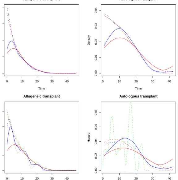
As for thef and λ functions, Figure 2 provides a plot of their presmoothed estimates. The selected plug-in and bootstrap bandwidths are also collected in Table2. The bootstrap selec-tor seems to give slightly large smoothing bandwidths b2, which entails smoother estimations
than those with the plug-in bandwidth selection. We also show how the estimates change depending on whether the boundary effect is corrected or not.
Here we only give details on theRcode run to get the estimates displayed on Figure2for the case off estimation in the ALLO group:
R> allo.f.pi <- presmooth(time, delta, allo, "f", "plug-in") R> allo.f.boot <- presmooth(time, delta, allo, "f", "bootstrap") R> allo.f.pi.bound <- presmooth(time, delta, allo, "f", "plug-in", + bound = "both")
R> allo.f.boot.bound <- presmooth(time, delta, allo, "f", "bootstrap", + bound = "both")
The estimates are computed at the points given by thex.estargument (see Table1). When, as in the previous lines of code, its value is not explicitly set,presmoothcomputes it internally. With the default value of x.est, estimation is done at a sequence of 50 equispaced points between the minimum and the 90th percentile of the observed times. As a guideline, density and hazard estimates at the right tail should be taken very cautiously due to their increased bias and variance.
A warning should be given about computing time, which is usually markedly longer for boot-strap than for plug-in bandwidth selection. Of course, this difference is due to the computer-intensive nature of bootstrap methods. On a machine with an Intel Core i7-3610QM processor and 7.7 GB of memory, the last two lines of code took respectively 3.372 and 14.857 seconds of CPU time.
Our bandwidth selectors for f and λ can be extended to the case without presmoothing, allowing the selection of plug-in and bootstrap smoothing bandwidths for the correspond-ing classical kernel estimators of these curves. For reference, the classical non-presmoothed estimates of f and λ thus obtained (with plug-in bandwidth selection) have been added to Figure 2 (and the values of the corresponding bandwidths to Table2). Forf, this estimate is computed by:
0 10 20 30 40
0.00
0.02
0.04
0.06
0.08
Allogeneic transplant
Time
Density
0 10 20 30 40
0.00
0.01
0.02
0.03
0.04
Autologous transplant
Time
Density
0 10 20 30 40
0.00
0.02
0.04
0.06
0.08
Allogeneic transplant
Time
Hazard
0 10 20 30 40
0.00
0.02
0.04
0.06
0.08
Autologous transplant
Time
Hazard
Figure 2: alloautodataset. Estimates of f (top panels) andλ(bottom panels), conditioned by type of transplant. Estimates were obtained with either plug-in (blue lines) or bootstrap (red lines) bandwidth selection, and without (solid lines) or with (dashed lines) correction of the boundary effect. The dotted black lines are non-presmoothed plug-in estimates off and λobtained with survPresmooth. The dotted-dashed green lines are alternative estimates of λcomputed with the Rpackage muhaz.
Forλ, the plot also shows the hazard estimates obtained with themuhazfunction inRpackage
muhaz, using the default settings for global bandwidth selection (local bandwidth selection, also possible with muhaz, is currently not available in survPresmooth). Note the clearly undersmoothed shape of the resulting hazard estimate in the AUTO group.
R> library("muhaz")
T C
Model αT βT αC βC π
I 1 4 1 5 0.48
II 1 0.7 0.25 0.9 0.73
III 1 4 0.8 4 0.71
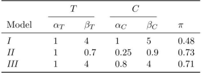
Table 3: Characteristics of the simulated modelsI,II and III.
Further aspects of the computation of the presmoothed estimates of S, Λ, f or λ can be fine-tuned by means of other arguments, including thecontrolargument and the associated
control.presmooth function. For example, the following code would compute the
pres-moothed estimate of S for the AUTO group with bootstrap bandwidth selected from a grid of 150 equispaced bandwidths between 1 and 50, taking B= 10000 bootstrap resamples, and a weight function with support on the interval defined by the 10th and 90th percentiles of the observed times:
R> presmooth(time, delta, auto, "S", "bootstrap", + grid.bw = seq(1, 50, length.out = 150),
+ control = control.presmooth(n.boot = 10000, q.weight = c(0.1, 0.9)))
5.3. Simulations
The practical performance of the presmoothed estimators and bandwidth selectors imple-mented in survPresmooth may be shown by means of simulation experiments. We have simulated four different models in order to describe the behavior in (non-cumulative and cu-mulative) hazard function estimation with varying sample size. For the sake of brevity, we do not give any results for survival and density functions. The models we have simulated try to define scenarios showing different combinations of purportedly influential conditions, like the intensity of censoring, the constant or non-constant nature of thep function, and the increasing, decreasing or non-monotonic nature of the hazard function.
In modelsI,II and III, both survival and censoring times follow a Weibull distribution with hazard function:
λ(t) = β α
t α
β−1
, t >0,
whereα and β are the scale and shape parameters.
The parameters characterizing the survival and censoring times of these models are collected in Table 3. Also shown is the value of the unconditional probability of censoring π = 1−
R∞
0 p(t)h(t)dt, whereh is the density of Z.
For model IV we have considered the distribution proposed byChen (2000). For parameters α >0,β >0, Chen’s hazard function is
λ(t) =αβtβ−1exp(tβ), t >0.
It can be shown thatλhas a bathtub shape forβ <1 and it is an increasing function forβ ≥1
Model I
0.00 0.10 0.20 0.30 0.40
0.20
Figure 3: Graphs ofp(black) andλ(red) for the simulated models. The dotted vertical lines identify the 20th and 80th quantiles of the observed time, which are the endpoints of the default weight function used for bandwidth selection bysurvPresmooth.
α= 1 andβ parameter equal to 0.7 and 1.2, respectively. For this choice, the unconditional probability of censoring is 0.41. Plots of thep and λcurves of models I–IV can be found in Figure3.
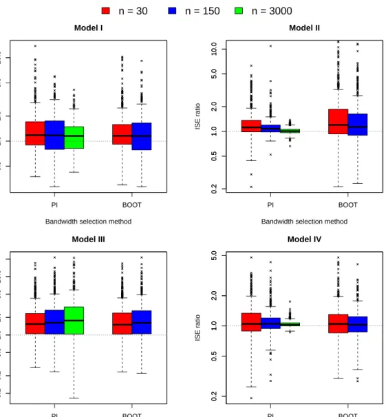
A total of 500 independent pseudorandom samples have been drawn from each model for small (n = 30), moderate (n = 150) and large (n = 3000) sample sizes. For each sample, presmoothed and non-presmoothed estimates of Λ andλ have been computed using, where applicable, our plug-in and bootstrap bandwidth selectors (actually, for n = 3000, due to computational burden, our experimentation has excluded the bootstrap bandwidth selector). For each simulated sample the integrated squared error (ISE) has been approximated by Simpson’s rule for numerical integration. For any bandwidth selector, let us denote by ISEP
the ISE of a presmoothed estimate and byISENP that of the corresponding non-presmoothed
0.5
Figure 4: Simulation results: box plots of theISENP/ISEP ratios for the non-presmoothed
and presmoothed estimates of Λ (for notation, see text). PI: plug-in bandwidth; BOOT: bootstrap bandwidth.
efficiency of presmoothed and non-presmoothed estimators. WhenISENP/ISEP takes a value,
say r, greater than 1, presmoothing is more efficient for that sample; more specifically, the presmoothed estimator is thenr times more efficient than the non-presmothed one.
0.05
Figure 5: Simulation results: box plots of theISENP/ISEP ratios for the non-presmoothed
and presmoothed estimates ofλ. Notation is the same as in Figure 4.
reason is that thepfunction of this model is constant, a condition where first order efficiency is attained (seeCao and J´acome 2004). As expected, the differences between both approaches tend generally to balance asn increases, but quite slowly, with the presmoothed estimators still being more efficient forn= 3000 in a majority of scenarios. The exception to this pattern is again ModelIII, where the ISE ratio seems to increase with n. This is hardly surprising since, as noted before, this model simulates a first order efficiency scenario. Overall, these results demonstrate the convenience of presmoothing, and the usefulness of thesurvPresmooth
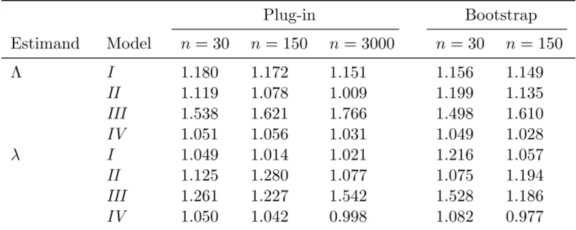
Plug-in Bootstrap
Estimand Model n= 30 n= 150 n= 3000 n= 30 n= 150
Λ I 1.180 1.172 1.151 1.156 1.149
II 1.119 1.078 1.009 1.199 1.135
III 1.538 1.621 1.766 1.498 1.610
IV 1.051 1.056 1.031 1.049 1.028
λ I 1.049 1.014 1.021 1.216 1.057
II 1.125 1.280 1.077 1.075 1.194
III 1.261 1.227 1.542 1.528 1.186
IV 1.050 1.042 0.998 1.082 0.977
Table 4: Simulation results: medians of theISENP/ISEP ratios for the non-presmoothed and
presmoothed estimates of Λ andλ(for notation, see text).
6. Conclusions
This paper deals mainly with the implementation inRof the presmoothed estimators of the survival, density, and cumulative and non-cumulative hazard functions of a right-censored lifetime. The new R package survPresmooth is introduced and described. Also, the theory underlying presmoothing has been summarized and further evidence showing the advantages of presmoothed estimators over their classical counterparts has been provided. Thepresmooth function of the package computes the presmoothed estimators in a user-friendly way. The function also implements two different methods for computing of the required bandwidths, based on bootstrap and plug-in techniques. Additionally, our software allows to compute well-known classical, non-presmoothed estimators (including, where applicable, their bandwidths), which may be interpreted as particular cases of presmoothed estimators.
There are several topics that are not dealt with by our package. We close the discussion with an enumeration of some of these issues, which give the opportunity for future developments of the package.
Although initially the graphical comparison of two or more distributions (straightforwardly done with survPresmooth) may be enough, hypothesis testing of the equality of survival distributions is more satisfactory from a statistical point of view. It is possible to adapt the log-rank test and, in general, all the weighted tests in the literature to the use of presmoothed estimators. However, these “presmoothed tests” remain largely unexplored and they should be carefully worked out before being implemented.
Our package does not provide confidence bands for the estimated functions. A way of con-structing them could be based on the bootstrap. The same resampling plan used for bootstrap bandwidth selection could be applied in order to compute the percentiles of the bootstrap dis-tribution of the estimates. The limits of pointwise confidence intervals could be constructed from these percentiles.
Sometimes, in addition to right censoring (RC), lifetimes are also subject to left trunca-tion (LT). The good properties of presmoothing are conserved in the so-called LTRC model:
see J´acome and Iglesias-P´erez (2008) for the case of S and Λ estimation, and J´acome and
Iglesias-P´erez (2010) for f. This suggests that, in principe, the procedures implemented in
Another issue not considered insurvPresmooth is the possible presence of covariates. Pres-moothing ideas are relatively new, and though survival analysis adjusting for covariates is of great interest, it has been scarcely investigated in the context of presmoothed estima-tion. For a semiparametric approach seede U˜na- ´Alvarez and Rodr´ıguez-Campos (2004) and
Iglesias-P´erez and de U˜na- ´Alvarez(2008).
Finally, let us point out that the properties of presmoothed estimators have been studied only in the setting of independent data, but in some studies survival times may be depen-dent. Under rather weak conditions for dependence, the KM estimator is still consistent and asymptotically normal (Ying and Wei 1994;Cai 1998). Similar ideas could be applied to try to prove that properties regarding consistency and asymptotic normality of the presmoothed estimators are also valid under the same weak conditions for dependence.
Acknowledgments
This research has been partially supported by the Spanish Ministry of Science and Innovation (Grant MTM2011-22392).
References
Aalen OO (1978). “Nonparametric Inference for a Family of Counting Processes.”The Annals of Statistics,6, 701–726.
Cai Z (1998). “Asymptotic Properties of Kaplan-Meier Estimator for Censored Dependent Data.”Statistics & Probability Letters,37, 381–389.
Cao R, J´acome MA (2004). “Presmoothed Kernel Density Estimator for Censored Data.”
Journal of Nonparametric Statistics,16, 289–309.
Cao R, L´opez-de-Ullibarri I (2007). “Product-Type and Presmoothed Hazard Rate Estimators with Censored Data.”Test,16, 355–382.
Cao R, L´opez-de-Ullibarri I, Janssen P, Veraverbeke N (2005). “Presmoothed Kaplan-Meier and Nelson-Aalen Estimators.”Journal of Nonparametric Statistics,17, 31–56.
Chen Z (2000). “A New Two-Parameter Lifetime Distribution with Bathtub Shape or In-creasing Failure Rate Function.” Statistics & Probability Letters,49, 155–161.
de U˜na- ´Alvarez J, Rodr´ıguez-Campos MC (2004). “Strong Consistency of Presmoothed Kaplan-Meier Integrals when Covariables Are Present.”Statistics,38, 483–496.
Dikta G (1998). “On Semiparametric Random Censorship Models.” Journal of Statistical Planning and Inference,66, 253–279.
Dikta G (2000). “The Strong Law under Semiparametric Random Censorship Models.” Jour-nal of Statistical Planning and Inference,83, 1–10.
F¨oldes A, Rejt¨o L, Winter BB (1981). “Strong Consistency Properties of Nonparametric Esti-mators for Randomly Censored Data. II Estimation of Density and Failure Rate.”Periodica Mathematica Hungarica,12, 15–29.
Gasser T, M¨uller HG (1979). “Kernel Estimation of Regression Functions.” In T Gasser, M Rosenblatt (eds.), Smoothing Techniques for Curve Estimation, volume 757 of Lecture Notes in Mathematics, pp. 23–68. Springer-Verlag.
Gasser T, M¨uller HG, Mammitzsch V (1985). “Kernels for Nonparametric Curve Estimation.”
Journal of the Royal Statistical Society B,47, 238–252.
Hess K, Gentleman R (2010). muhaz: Hazard Function Estimation in Survival Analysis. R
package version 1.2.5, URLhttp://CRAN.R-project.org/package=muhaz.
Iglesias-P´erez MC, de U˜na- ´Alvarez J (2008). “Nonparametric Estimation of the Conditional Distribution Function in a Semiparametric Censorship Model.”Journal of Statistical Plan-ning and Inference,138, 3044–3058.
J´acome MA (2005). Estimaci´on Presuavizada de las Funciones de Densidad y Distribuci´on con Datos Censurados. Ph.D. thesis, Universidade da Coru˜na.
J´acome MA, Cao R (2007). “Almost Sure Asymptotic Representation for the Presmoothed Distribution and Density Estimators for Censored Data.”Statistics,41, 517–534.
J´acome MA, Cao R (2008). “Strong Representation of the Presmoothed Quantile Function Estimator for Censored Data.”Statistica Neerlandica,62, 425–440.
J´acome MA, Gijbels I, Cao R (2008). “Comparison of Presmoothing Methods in Kernel Density Estimation under Censoring.”Computational Statistics,23, 381–406.
J´acome MA, Iglesias-P´erez MC (2008). “Presmoothed Estimation with Left-Truncated and Right-Censored Data.” Communications in Statistics – Theory and Methods, 37, 2964– 2983.
J´acome MA, Iglesias-P´erez MC (2010). “Presmoothed Estimation of the Density Function with Truncated and Censored data.”Statistics,44, 217–234.
Kaplan EL, Meier P (1958). “Nonparametric Estimation from Incomplete Observations.”
Journal of the American Statistical Association,53, 457–481.
Klein JP, Moeschberger ML (2003). Survival Analysis: Techniques for Censored and Trun-cated Data. Springer-Verlag.
Klein JP, Moeschberger ML, Yan J (2012).KMsurv: Data Sets from Klein and Moeschberger (1997), Survival Analysis. R package version 0.1-5, URL http://CRAN.R-project.org/ package=KMsurv.
L´opez-de-Ullibarri I, J´acome MA (2013). survPresmooth: Presmoothed Estimation in Sur-vival Analysis. R package version 1.1-8, URL http://CRAN.R-project.org/package= survPresmooth.
Nadaraya EA (1964). “On Estimating Regression.”Theory of Probability and Its Applications,
10, 186–190.
Nelson W (1972). “Theory and Applications of Hazard Plotting for Censored Failure Data.”
Technometrics,14, 945–965.
Parzen E (1962). “On Estimation of a Probability Density Function and Mode.”The Annals of Mathematical Statistics,33, 1065–1076.
Ramlau-Hansen H (1983). “Smoothing Counting Process Intensities by Means of Kernel Functions.”The Annals of Statistics,11, 453–466.
RCore Team (2013). R: A Language and Environment for Statistical Computing. R Founda-tion for Statistical Computing, Vienna, Austria. URLhttp://www.R-project.org/.
Rosenblatt M (1956). “Remarks on Some Nonparametric Estimates of a Density Function.”
The Annals of Mathematical Statistics,27, 832–837.
S´anchez-Sellero C, Gonz´alez-Manteiga W, Cao R (1999). “Bandwidth Selection in Density Estimation with Truncated and Censored Data.” Annals of the Institute of Statistical Mathematics,51, 51–70.
Stone M (1974). “Cross-Validatory Choice and Assessment of Statistical Predictions.”Journal of the Royal Statistical Society B,36, 111–147.
Tanner MA, Wong WH (1983). “The Estimation of the Hazard Function from Randomly Censored Data by the Kernel Method.”The Annals of Statistics,11, 989–993.
Watson GS (1964). “Smooth Regression Analysis.” Shankya A,26, 359–372.
Yandell BS (1983). “Nonparametric Inference for Rates with Censored Data.”The Annals of Statistics,11, 1119–1135.
Ying Z, Wei LJ (1994). “The Kaplan-Meier Estimate for Dependent Failure Time Observa-tions.”Journal of Multivariate Analysis,50, 17–29.
Affiliation:
Ignacio L´opez-de-Ullibarri Departamento de Matem´aticas Universidade da Coru˜na
Escuela Universitaria Polit´ecnica Ferrol, A Coru˜na, Spain
M. Amalia J´acome
Departamento de Matem´aticas Universidade da Coru˜na Facultad de Ciencias A Coru˜na, Spain
E-mail: [email protected]
Journal of Statistical Software
http://www.jstatsoft.org/published by the American Statistical Association http://www.amstat.org/
Volume 54, Issue 11 Submitted: 2011-03-21